Closed-loop Reference Model adaptive control : with application to very flexible aircraft

Closed-Loop Reference Model Adaptive Control:

with Application to Very Flexible Aircraft

by

Travis Eli Gibson

B.S., Georgia Institute of Technology (2006)

S.M., Massachusetts Institute of Technology (2008)

Submitted to the Department of Mechanical Engineering

in partial fulfillment of the requirements for the degree of

Doctor of Philosophy in Mechanical Engineering

at the

MASSACHUSETTS INSTITUTE OF TECHNOLOGY

February 2014

@

Massachusetts Institute of Technology 2014. All rights reserved.

"n-A u th o r ...

.

.

.

...

.

.

Department of Mechanical Engineering

December 30, 2013

Certified by...

Annd15i

M. Annaswamy

Senior Research Scientist

Thesis Supervisor

A ccepted by ...

....

1-

David E. Hardt

Chairman, Department Committee on Graduate Theses

MASSACHUSETS INSf'lEF OF TECHNOLOGY

MAY

L'8

2014

KLiBRARIES

Closed-Loop Reference Model Adaptive Control:

with Application to Very Flexible Aircraft

by

Travis Eli Gibson

Submitted to the Department of Mechanical Engineering on December 30, 2013, in partial fulfillment of the

requirements for the degree of

Doctor of Philosophy in Mechanical Engineering

Abstract

One of the main features of adaptive systems is an oscillatory convergence that ex-acerbates with the speed of adaptation. Over the past two decades several attempts have been made to provide adaptive solutions with guaranteed transient properties. In this work it is shown that Closed-loop Reference Models (CRMs) can result in improved transient performance over their open-loop counterparts in model reference adaptive control. In addition to deriving bounds on L-2 norms of the derivatives of the adaptive parameters which are shown to be smaller, an optimal design of CRMs is proposed which minimizes an underlying peaking phenomenon. The analytical tools proposed are shown to be applicable for a range of adaptive control problems including direct control, composite control with observer feedback and partial states accessible control. In addition a detailed study of the applicability of CRM adaptive control to very flexible aircraft is presented.

Following the NASA Helios flight mishap in 2003 there has been a push for greater understanding of the aerodynamic-structural coupling that occurs in light, very flex-ible, flying wings. Previous efforts in that direction revealed that the flexible aircraft had instability in the phugoid mode for large dihedral angles and that including the flexible dynamics was necessary to arrive at an appropriate trim condition. In this thesis, we show how these large dihedral excursions can occur in the presence of turbulence, by constructing an overall nonlinear model that captures the dominant dynamics of a very flexible aircraft. The thesis closes with the application of CRM adaptive control to the VFA model.

Thesis Supervisor: Anuradha M. Annaswamy Title: Senior Research Scientist

Acknowledgments

I would like to thank the scientific process for being true. The person most responsible

for my success is my advisor, Anuradha Annaswamy. Horror stories are passed around of inaccessible advisors, snap funding catastrophes and the like. She has always been available for discussion and has made sure that my funding was always in line, even during the economic crisis of 2008 and the sequestration in early 2013. Another person responsible for my success is Eugene Lavretsky. Eugene, like Anuradha, has always been accessible and was the one who encouraged me to study the specific adaptive structure that became the core of my thesis. I would also like to thank the other members of my PhD committee, Mark Drela and Jean-Jacques Slotine, for their valuable input. Colleagues that have positively influenced my work are Zac Dydek, Yoav Sharon, Yildiray Yildiz, Ross Gadient, David Wilcox, Irene Gregory, Sean Kenny and Luis Crespo. Finally, I have to thank my family: Eddie Gibson, for which hard work is his definition, Lisa Gibson, who made sure that I received the best education possible and even home schooled me when the local schools were not up to par, and Tyler Gibson for buying that motorcycle. If Tyler had not purchased a motorcycle and forced the big brother to man up I would have missed out on, whats is now, the biggest passion of my life. A very special thanks is in order for A.G. as well. I leave you with the most important statement made by an individual in my lifetime.

[Tjhe

offer of certainty, the offer of complete security, the offer of an impermeable faith that cant give way, is an offer of something not worth having. I want to live my life taking the risk all the time that I dont know anything like enough yet; that I haven't understood enough; that I cant know enough; that I'm always hungrily operating on the margins of a potentially great harvest of future knowledge and wisdom. I wouldn't have it any other way. And I'd urge you to look at those people who tell you, at your age, that you're dead till you believe as they do. What a terrible thing to be telling to children! And that you can only live by accepting an

absolute authority, dont think of that as a gift. Think of it as a poisoned chalice. Push it aside, however tempting it is. Take the risk of thinking for yourself. Much more happiness, truth, beauty, and wisdom will come

to you that way.

Contents

1 Introduction 1.1 Contributions by Chapter 2 Mathematical Preliminaries 2.1 Introduction . . . . 2.2 Preliminaries . . . . 2.2.1 Vector Norms 2.2.2 Matrix Norms 2.2.3 Signal Norms . . . 2.2.4 Positive Matrices . 2.2.5 Continuity . . . . . 2.2.6 Convergence . . . . 2.3 Definitions of Stability . . 2.4 Conditions for Stability . .

2.5 Linear Systems . . . .

2.5.1 Transfer Functions

2.5.2 Cheap Observer Ricca

and Stability Definitions

ti Equations

3 Closed-loop Reference Model Adaptive Control

3.1 Introduction . . . .

3.2 CRM-Based Adaptive Control of Scalar Plants . . . .

3.2.1 Stability Properties of CRM-adaptive systems . .

3.2.2 Transient Performance of CRM-adaptive systems

17 20 23 23 23 23 24 25 28 28 30 31 33 37 43 45 47 47 49 50 52

3.2.3 Effect of Projection Algorithm . . . .

3.3 Bounded Peaking with CRM adaptive systems . . . . .

3.3.1 Bounds on xm . . . ..

3.3.2 Bounds on parameter derivatives and oscillations

3.3.3 Simulation Studies for CRM . . . . 3.4 CRM for States Accessible Control . . . . 3.5 CRM Composite Control with Observer Feedback . . .

3.5.1 Stability . . . .

3.5.2 Transient performance of CMRAC-CO . . . . . 3.5.3 Robustness of CMRAC-CO to Noise . . . . 3.5.4 Simulation Study . . . .

3.5.5 Comments on CMRAC and CMRAC-CO . . . 3.6 CRMs in other Adaptive Systems . . . .

3.6.1 Adaptive Backstepping with Tuning Functions .

3.6.2 Adaptive Control in Robotics . . . . 3.7 Conclusions . . . .

4 Closed-loop Reference Models in SISO 4.1 Introduction . . . . 4.2 N otation . . . .

4.3 The Control Problem . . . .

4.4 Classical n* = 1 case (ORM n* = 1) . .

4.4.1 Stability for n* = 1 . . . . 4.5 CRM n* = 1 . . . . 4.5.1 Performance . . . . 4.6 CRM SISO n* = 2 . . . . 4.6.1 Performance . . . . 4.7 CRM Arbitrary n* . . . . 4.7.1 Stability for known high frequen 4.7.2 Performance when kP known .

Adaptive cy gain . Control 57 59 59 62 63 66 71 72 73 76 78 81 81 82 84 85 87 87 89 90 90 92 93 96 97 98 98 99 104

4.7.3 _{Stability in the case of unknown high frequency gain . . . 107}

4.8 _{C onclusion . . . 111}

5 Control Oriented Modeling of Very Flexible Aircraft 113 5.1 Introduction . . . 113

5.2 M odeling . . . 116

5.2.1 _{Vector Notation . . . .} 116

5.2.2 _{Forces and Frames for Aircraft Dynamics . . . .} 117

5.2.3 Linear and Angular Momentum for Very Flexible Aircraft . . 118

5.2.4 Forces and Moments acting on VFA in Stability Axis Frame . 122 5.3 Effect of Large Dihedral Angles . . . . 126

5.3.1 Trim Analysis . . . . 126

5.4 Control of Dihedral Angles . . . 129

5.4.1 Control Design . . . 129

5.4.2 Controllability and Observability . . . 131

5.4.3 Controllability and Observability Measures applied to VFA Model132 5.5 Analysis of Helios Crash . . . . 133

5.5.1 P art I: . . . . 134

5.5.2 P art II: . . . . 136

5.5.3 P art III: . . . . 137

5.5.4 P art IV : . . . . 138

5.6 C onclusions . . . . 138

6 Modern Output Feedback Adaptive Control 141 6.1 SISO: Zero Annihilation . . . . 142

6.2 MIMO Square: Zero Annihilation . . . . 145

6.3 MIMO LQG/LTR . . . . 148

6.4 Adaptive Control for Very Flexible Aircraft . . . . 151

7 Conclusions 163

7.1 Future W ork . . . . 163

A Projection Algorithm 165 A.1 Properties of Convex Sets and Functions . . . . 165

A .2 P rojection . . . . 167

A .3 F-Projection . . . . 172

B Bounds for Signals in SISO Adaptive System 173 B .1 N orm of ex(t) . . . . 173

B .2 N orm of ea(t) . . . . 175

C MIMO Adaptive Control Squaring Up Example 179 C.1 Creating SPR Transfer Functions for Square Systems Using Observer Feedback . . . .. 179

C .2 Squaring U p . . . . 181

C.3 Mixing the Outputs . . . . 181

List of Figures

1-1 Centrifugal governor [55].. . . . . 1-2 Open-loop reference model (top) does not use feedback from the error

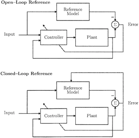
state to modify the reference trajectory. The closed-loop reference model (bottom) uses the error signal as an extra input into the reference m o d el. . . . .

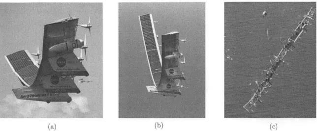
1-3 (a) Helios flying at normal dihedral. (b) Helios flying at large dihedral. (c) Helios breaking apart mid flight. . . . . Norm s in R2. . . . .

Asymptotic stability, adapted from [35]. Lyapunov stability, adapted from [35]. Asymptotic stability, adapted from [35]. Trajectories of the ORM

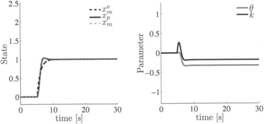
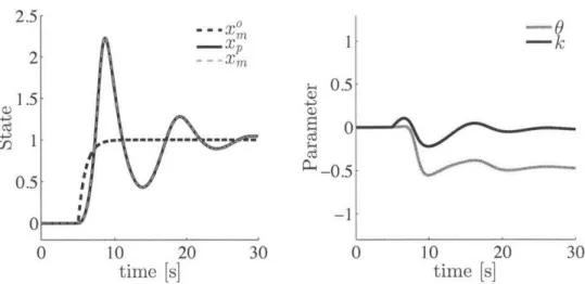
Trajectories of the ORM Trajectories of the ORM Trajectories of the CRM Trajectories of the CRM Trajectories of the CRM adaptive system y = adaptive system -y = adaptive system y = adaptive system y = adaptive system y adaptive system -y = 1. . . . . 10. .. .. ... 100 . . . . . . 100, e = -10. 100, f = -100. 100, f = -1000 17 19 20 24 32 35 36 . . . . . 64 . . . . . 64 . . . . . 65 . . . . . 65 . . . . . 65 . . . . 66 3-7 (top) reference model trajectories xm, (middle) state x, and (bottom)

m odel following e. . . . . 3-8 (top) Control input u, (middle-top) discrete rate of change of control

input Au/,At, (middle-bottom) adaptive parameter 0(t) and (bottom) adaptive parameter 0(t). . . . . 2-1 2-2 2-3 2-4 3-1 3-2 3-3 3-4 3-5 3-6 79 80

5-1 NASA Helios in flight. ... ... 114

5-2 Reference frames important for describing aircraft motion. . . . . 117

5-3 Artistic rendering of VFA. . . . . 118

5-4 Schem atic of VFA. . . . . 119

5-5 Eigenvalues for trim points. At zero dihedral angle the short period mode is lightly damped and the phugoid mode is stable. As the dihe-dral angle increases the short period mode damping increases and the phugoid mode becomes unstable. . . . . 128

5-6 Initial condition perturbation from trim input for dihedral angle of 5 degrees. . . . . 129

5-7 Helios flight mishap data (adapted from [651). . . . . 130

5-8 LQG Control Structure. . . . . 131

5-9 Measure of controllability as a function of input selection and dihedral an g le. . . . . 133

5-10 Measure of controllability as a function of input selection and dihedral angle, sem ilog plot. . . . . 134

5-11 Simulation in the presence of turbulence with At = 0.1 and D =1 for the three test case scenarios in Table 5.3. . . . . 136

5-12 Comparison of dihedral measured in ft for Helios mishap and VFA sim Case (i), D = 1, and At E {0.1, 0.05, 0.01}. . . . . 137

5-13 Comparison of dihedral measured in ft for Helios mishap and VFA sim Case (i), At = 0.1, and D c {1, N 5, V5 . . . . 138

5-14 Comparison of dihedral measured in ft for Helios mishap and VFA sim C ase (i). . . . . 139

6-1 PZ Map for MIMO system with feedback gain L chosen as in Lemma 6 .2 . . . . 1 4 5 6-2 Comparison of adaptive and linear controller to dihedral disturbance. 154 6-3 Comparison of adaptive and linear controller to dihedral disturbance t c [0 , 201. . . . . 156

6-4 Comparison of adaptive and linear controller to dihedral disturbance

t E [0 , 80j. . . . 157 6-5 Adaptive gains without turbulence t E [0, 801. . . . . 158 6-6 Comparison of adaptive and linear controller in the presence of

turbu-lence over t E [0, 20]. . . . . 159 6-7 Comparison of adaptive and linear controller to dihedral disturbance

in the presence of turbulence over t E [0, 800]. . . . . 160 6-8 Adaptive gains in the presence of turbulence t E [0,800]. . . . . 161

List of Tables

3.1 _{Test Case Equations . . . .} 79

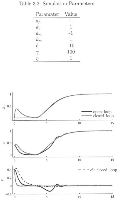
3.2 Simulation Parameters . . . . 79

5.1 Constants. . . . 126

5.2 Controllability/Observability Study . . . .. . . . . 133

5.3 Simulation Cases. . . . . 135

5.4 Simulation Cases. . . . . 135

6.1 Control Design Parameters. . . . . 155

Chapter 1

Introduction

Control systems arise anytime the output of a system needs to be regulated or forced to track a command. The first instances of control systems appeared in the first century A.D., in the form of water clocks.

[7]

The most cited modern example of a mechanical control system is that of the fly-ball governor, see Figure 1-1. [3] The fly-ball governor was first used to regulate the speed of the output shaft on a steam engine. The output shaft of the steam engine is connected to the shaft that the ball governors rotate on. As the speed of the output shaft increases, the the scissor arms spread, and the linkage at the top of figure then decreases the throttle setting on the righthand side of the figure. This illustrates the defining feature of automatic control, the notion of feedback. [80] That is, a system output is measured and then fed back

e n o

into the input of the system. Feedback control systems are ever-present occurring naturally or engineered into our machines.

The basic premise of any adaptive control system is to have the output of a plant follow a prescribed reference model through the online adjustment of control parameters. [4,32, 37,41,47, 61, 73] Adaptive control originated in 1958 [79] and was popular in aircraft control for most of the 60's until the X-15 flight mishap in 1967 [17,

251. It was clear that adaptive control was in its infancy and it would take two more

decades until the stability of adaptive systems was fully understood [18,26,58,62,63]. Following stability of adaptive control systems in the 80s and their robustness into the 90s [31, 36, 59, 60, 67], several attempts have been made to quantify transient performance (see for example, [10, 38,81]).

Historically, the reference models in MRAC have been open-loop in nature (see for example, [32, 61]), with the reference trajectory generated by a linear dynamic model, and unaffected by the plant output. The notion of feeding back the model following error into the reference model was first reported in [49] and more recently in [20-23, 44, 45, 74, 75]. We denote adaptive systems with an Open-loop Reference Model as ORM-adaptive systems and those with closed-loop reference models as CRM-adaptive systems, see Figure 1-2.

Combined/composite direct and indirect Model Reference Adaptive Control (CM-RAC) [16,72], is another class of adaptive systems in which a noticeable improvement in transient performance was demonstrated. While the results of these papers estab-lished stability of combined schemes, no rigorous guarantees of improved transient performance were provided, and have remained a conjecture [43]. This thesis is con-cerned with rigorously proving how one can design CRM adaptive systems with im-proved transient performance over their ORM counterparts.

In keeping with tradition our application of interest is that of aircraft control. Re-cently the control of very flexible aircraft has become of interest. One such example is the Helios aircraft, depicted in Figure 1-3. On June 2 6th 2003 the aircraft broke apart

mid-flight during testing. Throughout the flight the aircraft encountered turbulence. After approximately 30 minutes of flight time a larger than expected wing dihedral

formed and the aircraft began a slowly diverging pitch oscillation. The oscillations never subsided and led to flight speeds beyond the design specifications for Helios. The loading on the aircraft compromised the structure of the aircraft and the skin of the aircraft pulled apart. One of the key recommendations that came from the flight mishap investigation was to, "Develop more advanced, multidisciplinary (structures, aeroelastic, aerodynamics, atmospheric, materials, propulsion, controls, etc) "time-domain" analysis methods appropriate to highly flexible, "morphing" vehicles" [65].

This thesis addresses this recommendation directly with a control oriented model of very flexible aircraft and an adaptive control design.

The thesis is organized as follows: Chapter 2 contains the mathematical prelimi-naries, Chapter 3 contains the main theoretical components of transient response and CRM systems, Chapter 4 analysis's the benefits of CRMs in SISO adaptive control, Chapter 5 presents a model for control design of very flexible aircraft, Chapter 6

con-Open-Loop Reference 0 Reference Model Error Input _Controller - Plant Closed-Loop Reference Reference Model E Error Input _Controller - Plant

Figure 1-2: Open-loop reference model (top) does not use feedback from the error state to modify the reference trajectory. The closed-loop reference model (bottom) uses the error signal as an extra input into the reference model.

(a) (b) (c

Figure 1-3: (a) Helios flying at normal dihedral. (b) Helios flying at large dihedral. (c) Helios breaking apart mid flight.

tains the adaptive control design for very flexible aircraft, and Chapter 7 ends with conclusions and future directions.

1.1

Contributions by Chapter

Chapter 2

Very little in this chapter is original. All of the definitions pertaining to real analysis were taken from [69]. The functional analysis results were taken from MIT 18.102 course notes. The stability definitions originated in [52] with the necessary conditions from stability coming from [51,61].

Chapter 3

The main contribution of this thesis comes in this chapter. It is shown how one can design adaptive systems with improved transients in terms of model following error and a reduced L-2 norm of the derivative of the adaptive parameters. It is then shown that reducing the L-2 norm of the derivative of a signal directly correlates into a reduction of the high frequency oscillations of the system. Another major contribu-tion from this chapter is the introduccontribu-tion of adaptive systems with filtered regressor

vectors. It is shown that introducing CRMs into CMRAC results in the recovery of a separation like principle.

Chapter 4

This chapter extends the results of Chapter 3 to the SISO case. There are three con-tributions from this chapter: 1) Using CRM, one can follow reference models that are not SPR. 2) Using CRMs in SISO control one can choose the feedback gain such that the error model reduces to a first order decay, 3) Analysis of adaptive systems always comes in the form of non-minimal state analysis. This chapter illustrates that much tighter performance bounds can be achieved when analyzing the minimal state-space models. This chapter also shows that the results for the scalar adaptive system in Chapter 3 were not a fluke.

Chapter 5

This chapter introduces a first principles simple model of very flexible aircraft. A trend in the literature surrounding VFA is that complicated CFD models are needed to explain why the Helios flight mishap occurred. However a simple understudying of controllability could have predicted the demise of he Helios aircraft. It is shown through simulation that VFA can suffer from turbulence induced dihedral drift, the

catalyst for the Helios crash.

Chapter 6

This chapter analyzes a modern interpretation of output feedback adaptive control. This is accomplished via a zero annihilation technique and an LQG/LTR technique

first realized in [44]. A different stability analysis is presented for the LQG/LTR

technique as compared to that in [47] where limt, e(t) = 0. Also, the need for a

of LQG/LTR adaptive control to the VFA model presented in Chapter 5.

Chapter 7

Chapter 2

Mathematical Preliminaries and

Stability Definitions

2.1

Introduction

This chapter introduces the basic mathematical principles and theorems necessary to discuss the stability and transient performance of adaptive systems.

2.2

Preliminaries

2.2.1

Vector Norms

A norm on a vector space V, usually denoted as

,

maps from a vector space V to the real numbers and is always greater than or equal to zero. Our vector spaces of interest are R" (vectors containing all real elements) and possibly Cn (vectors of complex elements).

Definition 2.1 (Norm). V is a vector space over the field K. Let the norm be defined

as |I-I| : V -+ [0, oo). Let a E K and x, y E V. All norms satisfy (a) ||xfl= 0 if and only if x = 0

(c) 1|x + y < ||4|+ |y1|

With the following subscript definition,

xT = [xi

for all x E R, n I P < 0c

(i4

and

flx1'Oo sup

1xil

.

The norms are referred to as p-norms (1-norm, 2-norm, ... , oc-norm). It will always

be assumed that when the subscript on the p-norm is not given, we are assuming

p = 2,

||xHI J |XH2.

A visualization of these norms is given in Figure 2-1.

X1 IIXI12 ^

|14

₀₀

Figure 2-1: Norms in R2

2.2.2

Matrix Norms

Let A E R"'mX then the induced p-norm is defined as S |Axfll ||Allp = sup . 11X11=1 ||x4| X2 ... xn n / = 1 \ p

when the Euclidean norm is used, i.e. p = 2 we have that

|A 2 = \/Amax (ATA)

where Amax denotes the maximum eigenvalue. Also as before, when no p value is denoted, it is assumed that p = 2,

||A|| =

||A||2-Property 2.1. The induced p-norms have two special properties. Let x G Rn, A C Rmxn and B e R nxd

Il~ x l p < IJ A l pl~ ~ l p(2 _{.1 )}

Note that this property need not hold for all matrix norms.

Definition 2.2. When a norm satisfies the second property above,

||AB|

, <

||A|l|lIB |

it is called a sub-multiplicative norm.

Definition 2.3. Let A (E Rn x n , the Frobenius norm is defined as

||A||F = trace(ATA)

Property 2.2. The Frobenius norm is a sub-multiplicative norm.

2.2.3

Signal Norms

Let x(t) :R --+ R' and 1 p < oo i/p Jx(t) |LP (2.2)

t

tlim jx(T JjdT and

||X(t)Lo -,A sup x(t)I| t

Note that we are not using the essential supremum here, but just the supremum.

If the essential supremum were being used, then we would allow the signal to be

unbounded on a set of measure zero, and it would still be in Co. With our definition, if a signal is in Lo then the signal is bounded for all time.

The above norm is called the Lp-norm. The p-norm was used on a time varying signal x(t) giving us a time dependent "norm" 11x(t)JI. At each fixed t, 1x(t)J| is a norm, but it is not true to say that for all t, IIx(t) is a norm. We need a scalar value for all t, so we resorted to integration or using the supremum operator. The above definitions also hold for the induced matrix norms.

It is notationally equivalent to write Lp, LP, L,, LP. Its just a preference of superscript, subscript, and or calligraphic text.

Lemma 2.1. For a, b 0 and t E [0,1] the following holds

eta+(1-t)b < tea + (1 - t)eb.

Proof. This proof follows from the fact that the exponential function is concave up

and any secant line is always necessarily above the exponential function between the two points of intersection.

Theorem 2.1 (Young's Inequality). For ab > 0 and p, q > 1 the following holds

av bG a b < -P + --p q where 1+1 -+- = 1. p q

Proof. Begin with the equality

ab = eloga+logb

Ip log a+1 q log b

From the fact that 1/p = 1 - 1/q and using Lemma 2.1 we have that ab < 1 ploga+ e qlogb p q 1 a + 1b p q E

Theorem 2.2 (Hoelder's Inequality). Let f(t) and g(t) be scalar

functions

of time with bounded LP and Lq norms respectively where 1 = 1p

+

1/q, then

1Li < g(t) f(t) LT Lq

Proof. Starting with the triangle inequality we have

|f(t) Lpjg(t) Lq f(t) Lp |g(t)|Lq

Application of Theorem leads to

(2.4)

||f(t) p g(t)j Lq -Kf(t) L/

Integrating both sides we have

f (t)g(t)j|dt <

+ (

1g(O'>l

_{11(t) | L,}

)

q

h1-

(

_{1f |(t)||Lp}

fM1

)P

p q

= 1.

Multiplying both sides by ||f(t)jjLpjjg(t)||Lq gives us the result.

Proposition 2.1 (Cauchy-Schwarz Inequality). Holder's inequality with p = 2.

dt dt + j 11|g(t)| 11

q 19(t L,

2.2.4

Positive Matrices

Definition 2.4. A matrix M E R"' is positive definite if zTMz > OVz # 0 and is

often denoted as M > 0.

Lemma 2.2. Let M be a symmetric matrix with the following decomposition:

A B

M =

LBT C

A = AT and C = CT is full rank. M > 0 if and only if

C> 0

SA- BC-lBT > 0

Proof. Given that C is full rank, the inverse of C exists and therefore the following

relation holds

BC-1 A - BC-1BT

I 0

0

I

BC-1

C0 I]

A block diagonal matrix is positive definite iff all diagonal blocks are positive definite.

This concludes the proof, thus M > 0 off C > 0 and A - BC-BT. D

2.2.5

Continuity

We start with the definition of a metric space.

Definition 2.5 (Metric). A set X whose elements are called points, is said to be a

metric space, if with any two points p and q in X there is associated a real number

d(p, q), called the distance from p to q, such that

* d(p,q) > 0if p 7q ;d(p, p) =0 * d(p,q) = d(q,p) * d(p,q) < d(p,r) + d(r,q), for any r E X B] C A BT [0

A function with these three properties is called a distance function or a metric.

Note that a norm on any subset of the real or complex numbers is a metric, but not all metrics are norms. Norms have two extra properties as compared to distance functions, and those are translation invariance and scaling.

Definition 2.6 (Limit Point). Let X and Y be metric spaces; supposes E C X, f

maps E into Y, and p is a limit point of E,

lim f (x) = q x--+p

if there is a point q E Y with the following property: For every e > 0, there exists a

j > 0 s.t.

dy (f (x), q) < c

for all points x G E for which

0 < dx(x,p) < 6

where dx and dy are distance functions in X and Y respectively.

Definition 2.7 (Continuity). Let X and Y be metric spaces; supposes E C X, p C E

and

f

maps E into Y. Then

f

is continuous at p, if for every c > 0 there exists a

6 > 0 such that

dy(f(x), f(p)) <e

for all point x

c

E for wich d,(x, p) < 6.

Definition 2.8 (Uniform Continuity). Let

f

be a mapping of a metric space X into a metros space Y. If for every c > 0 there exists a 6 > 0 such that

dy (f (p), f (q)) <6 for all p and q in X for which d.(p, q) < 6.

2.2.6

Convergence

Theorem 2.3. Let {pn} be a sequence in a metric space X. Then,

1. {Pn} converges to p c X iff every neighborhood of p contains all but finitely many of the terms of {pn}.

2. If p e X and p' G X and if {pn} p and {pn} -+ p', then p = p'.

3. If {Pn} converges, then {pn} is bounded.

4. If E C X and if p is a limit point of E, then there is a sequence {Pn} E E such that p = limn_,oo pn

Theorem 2.4. Suppose {sO} is monotonic. Then

{s}

converges iff it is bounded.

Proof. Suppose s, < sn+1 . Let E be the range of

{sn}

If

{s4}

is bounded, let s be the least upper bound of E. Then sn < s and for every c > 0, there exists and integer N such that s - e < sN < s for otherwise s - e would be the least upper bound of E. Since {s} increases, s - e < sn s, Vn > N, which shows that {sn} converges to

s. The converse follows from Theorem 2.3. El

Definition 2.9. A sequence of functions

{fn(x)},

n = 1, 2, 3, ... converges point wise

on set E to

f,

if for each x E E there exists an E(x) such that n > N implies

|lf (X) - fn(X)| 1 <-E.

The convergence is uniform if e is independent of x.

Theorem 2.5. Suppose fn -+ f uniformly on a set E in a metric space. Let x be a

limit point of E, then

lim lim fn(t)

t-+x n-+oo

= lim lim fn(t)

n-*oo t-+x

Li

2.3

Definitions of Stability

Consider a dynamical system of time, t E R, varying state x E R. satisfying

X(to) = Xo

±(t)

= f

((t), t).

We are only interested in systems with equilibrium at x = 0, so that f(0, t) = 0 Vt.

The solution to the differential equation in (2.5) is a transition function O(t; xo, to) such that

O; Xo, to) = Xo. (2.6)

Below we give the various definitions of stability as defined in [27, 35,52,61]

Definition 2.10 (Stability). Let to > 0, the equilibrium is

(i) Stable, if for all e > 0 there exists a 6(e, to) > 0 s.t. _{|Hxojj < J implies} (to; to, Xo) 1 e V t > to.

(ii) Attracting, if there exists a p(to) > 0 such that for all q > 0 there exists a

T(q, xo, to) such that ||xo < p implies 11#(t; xo, to)| :5 q for all t > to

+

T.

(iii) Asymptotically Stable, if it is stable and attracting, see Figure 2-2.

(iv) Equiasymptotically Attracting, if the T in (ii) is uniform in xo and takes the form T(, p(to), to).

(v) Equiasymptotically Stable, if it is stable and equiasymptotically attracting.

(vi) Uniformly Stable, if the 6 in (i) is uniform in to, thus taking the form 6(c).

(vii) Uniformly Attracting, is equiasymptotic attracting where the p, T do not depend on to.

(viii) Uniformly Asymptotically Stable, (UAS) if it is uniformly stable and uniformly attracting.

(ix) Exponentially Asymptotically Stable (EAS) If the there exists a v > 0, and for

all ( > 0 there exists a 6(() such that

Hjxoj|

< 6 implies that ||#(t;xo,to)j| <

(e-"('-0) [52].

(x) Exponentially Stable If the there exists a v > 0 and p > 0 such that 110(t; xo, to)

p jxojje-v(-O)0

Definition 2.11 (Topology of Stability). The following define the neighborhoods

around the equilibrium for which the stability results hold.

(i) Global, if the results hold for all xo.

(ii) Local, if the results only hold for xO in a neighborhood around the equilibrium.

(iii) Semi-global, if the results hold globally for only a subset of the state space and locally for the other subset of the state space.

F 2to + T

to

2.4

Conditions for Stability

Consider dynamics of the form

i = f (t, x), x(to) = xO. (2.7)

where f(0, t) = 0 Vt > 0.

Theorem 2.6 (Lyapunov's Direct (The Second) Method). The equilibrium state of (2.7) is uniformly asymptotically stable in the large if a scalar function V(x, t) with

continuous first partial derivatives with respect to x and t exists such that V(O, t) = 0

and if the following conditions are satisfied

1. V(x, t) is positive definite, i.e. there exists a non-decreasing scalar function cz

such that a(O) = 0 and, for all t and all x

$

0

0 < a (11xII) < V(X, t)

2. There exist a continuous scalar function -y s.t. -y(0) = 0 and the derivative

V

of V along all system directions, satisfies for all t

X =

j+

(VV)Tf(x,t) -y ( 1x) < 0, Vx 4 0. at

3. There exist as a continuous non-decreasing scalar function such that 0(0) = 0

and for all t

V(x, 0 < 0 O||x||D

This is commonly referred to as "V is decrescent" (western literature) or "V has an infinitely small upper bound" (Russian literature).

4.

lim --oo

3(11

x ) = o

2.6.2 it follows

V (#(t; xo, to), t) - V(xo, to) =

J

1(0 $( ; xo,to),T )dT < 0,

and thus V is strictly decreasing along any trajectory.

Proof of uniform stability: For any c > 0 there exists a 6(c) such that 0(6) < a(c),

see Figure 2-3. Therefore, if f|xoJ| 5 6 where to is arbitrary, from 2.6.2 and (2.8) it follows that

a(G) > t(6) > V(o, to) ;> V(#(t; v, to), t) > a(wha(t; th, to)fli).

Given that a is positive and nondecreasing, we have the following,

||#(t; xo,to)|| < C V t > to, ||x<|| < 6,

for arbitrary to. Thus we have proved uniform stability.

Proof of uniform asymptotic stability: From Theorem 2.6.2, for any constant ci > 0

there exists an r > 0 such that O(r) ac(ci). For any xo such that

||xol

< r, by

uniform stability,

||#(t;

xo, to)J| < ci for all t > to, where to is arbitrary. For any

0 < p <

||xoHJ,

_{there exists a v(p) > 0 such that O(v) < a(pa), see Figure 2-3.}

Set c2(A, r) as the minimum of the continuous function 'y( |xJ) on the compact set

v(p) < ||xJ| < ci(r), and define T(p, r) A /(r)/c 2(P, r) > 0. Now assume for proof

by contraction that I

#(t;

xo, to)II > v over the interval to < t < ti = to + T. From

2.6.2 and (2.8) it follows that

0 < a(v) <V(0(ti; Xo, to), t1)

V(xo, to) - (ti - lo)c2

1(r) - Tc2 = 0.

Therefore, for some t = t2 in the interval [to, ti], it follows that lIX211 = 11#(t; £o, to) = (2.8)

v. Therefore

Ce(O X(t;x2,t 2) ,t)

V(x 2, t2) (v) < a()

for all t > t2. Therefore,

I(t; xo, to) < p V t > to + T(p, r) > t2, flXolI < r

which is the definition of uniform asymptotic stability.

Proof of uniform asymptotic stability in the large: From Condition 4 in Theorem

2.6, the r in the proof of uniform asymptotic stability can be arbitrary large. Uniform

boundedness also holds. D

O(I|x 1)

V(x, t)

0 6e

/e

/6

V =a(e) -x ~

Figure 2-4: Asymptotic stability, adapted from [35].

Proposition 2.2. If V(x, t) in Theorem 2.6 is positive definite and /(x, t) < 0, then

x(t) is bounded for all time.

Proof. Given that V is negative semidefinite, V(x, t) < V(xo, to) < oc. From the fact

that V(x, t) is positive definite it follows that ||x(t)|| < 00.

Lemma 2.3. If

f

: R+ -- I R is uniformly continuous for t ;> 0 and if

rt

lim t-+0 _fo~ El If(-r)|I < oo thus f(t) E C1, then lim f (t) = 0.

Proof. See [61, Lemma 2.12] _E

Corollary 2.1. If g C £2 0 £m and j is bounded, then limt_, ₀ g(t) ₌ 0.

Proof. Choose f(t) = g2(t) and the conditions of Lemma 2.3 are satisfied. _II Lemma 2.4. If g E L2 and j is bounded, then limtO g(t) = 0.

Proof. This follows by contradiction. Assume limt,, e(t)

$

0. Then there exists an

infinite unbounded sequence {tn}nEN and E > 0 such that Je(tj)| > E. And because

e

is bounded, e is uniformly continuous, and so Ie(t) - e(ti)| < kIt - tI V t, t c R+

for some k > 0, and we have e(t) > E - le(t) - e(ti)l. inequality

le(ti)l2 - 21e(t) - e(ti)|2 < 21e(t) 2

and integrate both sides from tj to t2 + 6 ti+62 (e(ti))2 dT- 2 t +6 (e (T) - e(ti))2 dr < 2

_ti

t+6 Ie(-) 2_dr.

Substituting in e < le(ti)l and the definition from uniform continuity

k2

(T _ t)2dT

J

fti - 2 _{(e(I) _ e(t- ))2} ,

t +6

E 2 dT- _{2k 2 i}

Integrating the left hand side

fI

t. ±3 2- _{k2 (3} K

Choosing 6 = ',

|e(T)|2dT >

Taking the limit as 6 -+ oc implies that limt,, f Ie(T) 2dT is not finite. This con-tradicts the assumption that e E L2and so we have limte, e(t) = 0. E

2.5

Linear Systems

Definition 2.12. A matrix A E R"'> is Hurwitz if all the eigenvalues of A are in

the open left half plane of C.

Theorem 2.7 (Lyapunov Equation). A E R"X"n is Hurwitz if and only if, for any

i

tj ± t and thus

ti

tj + t(+6 (2 - 7i+ t2)dr 2 T -2Fti ) d _{2 ti} |e(T)| 2_dT. e(T) 2dT. 6

Q

= QT > 0 there exists a unique P pT > 0 satisfying

ATp + PA = -Q. (2.9)

Proof. See [61, Theorem 2.10]

Example 2.1. The linear system

J(t) = Ax(t)

E

(2.10)

where x

E

R" and A

c

Rn>< is Hurwizt, is uniformly asymptotically stable in the large. This can be proved as follows: Consider the Lyapunov candidate

V(x, t) = x(t)TPX(t).

Taking the time derivative along the system trajectories in (2.10) results in V(x, t)

-x(t)T (ATP + PA)x(T). Using Theorem 2.7 we have

V(x,t) = -x(t)T Qx(t).

From Theorem 2.6, x = 0 is uniformly asymptotically stable in the large.

Consider the linear time-varying system

±(t) = F(t)x(t), (2.11)

which has solutions

#(t; Xo, to) = (b(t, to)xo, (2.12)

where (D is the state transition matrix.

Theorem 2.8. Given the system dynamics in (2.11), the following three statements

are equivalent

(b) The system is exponentially asymptotically stable.

(c) The system is exponentially stable.

Proof. This proof follows from [35, Theorem 3]. For any system, (c) -+ (b) -+ (a)

trivially. We now prove that (a) implies (b). Given that uniform asymptotic stability implies uniform stability we note that for all e > 0, 0 <

||xoll

< 6(e) which by linearity in (2.12), implies that

6-1 | (t;xot o)| :5 1(tto)l3-1 Xoll < /1#(t,to)l| < 6-e (2.13)

By uniform asymptotic stability choose T(2-, 1) so that 1(to + T, to) < 1/2

inde-pendent of to. It can be shown by induction that

||4D(to + kT,to)l| <1|4b(to + kT to + (k - 1)T||| ...

|1(to

+

T, tol (2.14)

Therefore we have that

|1(t,to)|| < 263ee 1o2) (t to)

In order to prove that this is the same as Exponential Asymptotic Stability, =2-1

and v = log(2)T- 1. Note that T is a fixed constant and therefore V is a constant for all initial conditions. Given that the dynamics in (2.11) are linear, in order for stability to hold, there must exist a finite upper bound on 1 independent of t. Therefore, for all c > 0, there exists a p such that 26 1e < p < oc. This completes the proof. El

Example 2.2. Consider the scaler dynamical system

where

c(x) =

if x do

else

The system is globally uniformly stable, but only locally uniformly attracting. There-fore, the system is not Exponentially Stable. For all ( > 0, define

if ( < do else

Thus, for all jxo| < 6 ,

| (t; xo, to)II < (e-(t-to).

Therefore, the system is Exponentially Asymptoticaly Stable.

Example 2.3. Consider the time response of the dynamical system x(t) E R' and

u(t) E

R,

- (t) = Ax(t) + bu(t) (2.15)

where A is Hurwitz and further more we are told that u(t) E L2, i.e. there exists a

c1 > 0 such thatItU(t)I L2 < c₁ < oo. Given that A is hurwitz, there exists _{c2, c}

3 > 0

such that

e At|l < c2e-3t. (2.16)

Details on bounding the matrix exponential can be found in [57].

response of x(t) is

x(t) = e Atx(0) +

e

A(-7-)u(TF)dT

The time series

(2.17)

Using the bound in (2.16) and taking the 2-norm for fixed t we have

IIx(t)

5 c2e C3tx(0) +

I

t

c2eC3 (t-T) Ilu(T) ~dT. (2.18)

Using Holder's inequality on the last term we have that

IIx(t)H 5 c2e -3 tx(0) + c 2e- 2c3(t--r)dT u(T) 2dr.

Using the bound given to us for u(t) we can say

jx(t)l < c2e tx(O) + cIc2

j

e- 2c3(tr)d.(2.20)

Lemma 2.5 (Gronwall-Bellman). For u, v > 0 and c1 a positive constant, and if

u(t) < C1 + t

u (-F) v(-)dr (2.21)

then

u(t)

<

cieftV(T)d-.

Proof. From (2.21) we have

u(t)v(t)

< V(t). c1 + fJ' ur)v()dr<vt).

Integrating both sides between 0 and t we have

u()v(T)dr) - log c1 <

li

v(T)dr.

Adding log ci to both sides and taking the exponent we have

U (T)V(T)dTr c efo v(,)d,

Theorem 2.9. The scalar dynamical system described by

S= (a + b(t))x

with a < 0, b

C

L2 results in bounded trajectories for x.

(2.19)

log (c

+

U(T) < c +

Proof. The solutions to (2.22) is

x(t) = eatx(0) + ea(t-r)b(Tr)x(T)dT.at

First note that e'tx(O) < x(O), then we can conclude that

x(t) < x(0) +

I

tea(-T) b(T) X(T) dT,

and taking 2-norms

x(t) < 1x(0)H1 + e"(t _{)b() x(r)||dr,}

Applying Lemma 2.5 where

ci =H1x(0)1|

U

=||x()br)

V =I|e aktTs(T b results in

||x(t)J| ||x(O)||efIIea(tT)b(T)IdT

<

||x(0)||efoI$ al-rIII ()Id Application of Cauchy Schwarz inequality results in

|1x(0|1 <- ||x(0 )||e fo lletatt-r 24d, S 2lb 4,l~-T

The quantity f ea(t-T) ₀ 122 d7< d1 and we are told that b E L ₂. Thus

- 21al

Tx(t)uf sub(iose wl 2ak

baseline example:

(t) =Ax + Bu _y = CTx (2.23)

where x E R', y C Rm and u C RP with A, B, C of appropriate dimension in the reals. The transfer function is then defined as

Z(s)= CT(sI - A)- 1B. (2.24)

2.5.1

Transfer Functions

Definition 2.13. A rational transfer function H(s) is a transfer function defined as

H(s) = p(s)/q(s) where p and q are polynomials.

Definition 2.14. A rational transfer function H(s) is analytic in Q if H(s) is bounded

for all s C Q.

Definition 2.15. Given a transfer function H(s) = (amsm +- + ais + ao)/(bns" + - + bis

+

bo) the relative degree is defined as

n* A -- m

Definition 2.16 ( [33]). A rational function H(s) is Strictly Positive Real (SPR) iff

" H(s) is analytic in Re[s] > 0,

" Re[H(jw)] > 0 V w E (-oo, oc) and,

* lim2a0 w2Re[H(jw)] > 0 when the relative degree is 1. When n* = 0 the third condition is not needed.

Lemma 2.6 (Meyers Kalman Yakubovich (MKY)). Given a scalar y > 0, vectors b

and h, and asymptotically stable matrix A, and symmetric positive-definite matrix L,

if

then there exists a scalar E > 0, a vector q and P = PT > 0 such that ATP + PA = -qqT - L

Pb - h = Iyq.

Proof. See [61, Lemma 2.4] E

Lemma 2.7 (Anderson Kalman Yakubovich (AKY)). Define Z(s) = cT(sI - A) 1b.

The poles of Z(s) satisfy Re[s] < -p. Z(s) is SPR iff there exists P = pT > 0 and L s.t.

ATP+PA=-LL _-_PP =-Q

Pb = c.

Proof. This follows from Lemma 2.6

Definition 2.17. The matrix pencil of the triple {A, B, C} for the system in (2.23)

is defined as sI-P~s)=- CT A - B 0 (2.25)

Definition 2.18. The transmission zeros of Z(s) in (2.24) are defined as the set

Zt= {s rank P(s) < n + min(m,p)}

where P(s) is the matrix pencil of (2.23) defined in (2.25)

Lemma 2.8. If the system in (2.23) is square (p=m), and CTB is full rank, then

there are exactly n - m transmission zeros.

Proof. See [11]. L

F-2.5.2

Cheap Observer Riccati Equations

Consider A E R"'f and B, C E R"' where (A, CT) is observable.

Q>

0 in R" and Ro= RT > 0 in R"m and for all vi> 0, with

For any Qo =

Q = Qo + (1 +1) BBT, R- V Ro

v + I

the solution P, = P > 0 to the well known observer Riccati Equation:

- (1+1- PvCR-lCTPV + Qo + (1 ₊ )BBT = 0

always exists. Another way of representing the Riccati Equation when the 1/v terms are collected is given below

PAT + AP, - PCROCTPV + Qo + BBT +I (BBT - PvCROCTP,) = 0

V

(2.27)

If in addition we assume that the transfer function Z(s) is minimum phase and CTB

is full rank. Then it is well known that the asymptotic expansion

P, = Po + P1l + 0(v2) (2.28)

approximates P, with P = POT> 0. That is lim,,o P, = P and is positive definite,

even in the limit of a cheap observer, i.e. v goes to 0.

[40]

Theorem 2.10 (Corollary 13.1 to Theorem 13.2 in [47]). For the triple {A, B, CT},

minimum phase, fully observable, square and CT B full rank

1. P and P are symmetric positive definite.

2. There exists a unitary matrix W E R"'xm such that

PoC = BWT &R

(2.29)

C = PoBWT R~

PoB - CRO11 2W

where Po = P 1 _{and W = (UV)T with}

BT CRO/ = UzV.

3. The following two asymptotic relations hold: PC = BWT Ro + O(v) C = P!BWT VRo + O(v) 5,B = CRO-1 1 W + O(v) where P, = P,-' Proof. See §13.3 in [47]. (2.30)

Chapter 3

Closed-loop Reference Model

Adaptive Control

3.1

Introduction

A universal observation in all adaptive control systems is a convergent, yet oscillatory

behavior in the underlying errors. These oscillations increase with adaptation gain, and as such, lead to constraints on the speed of adaptation. The main obvious chal-lenge in quantification of transients in adaptive systems stems from their nonlinear nature. A second obstacle is the fact that most adaptive systems possess an inher-ent trade-off between the speed of convergence of the tracking error and the size of parametric uncertainty. In this chapter, we provide a solution to this long standing problem, and overcome these challenges by proposing an adaptive control design that judiciously makes use of an underlying linear time-varying system, and introduces

design changes that decouple speed of adaptation from parametric uncertainty. The basic premise of any adaptive control system is to have the output of a plant follow a prescribed reference model through the online adjustment of control parame-ters. Historically, the reference models in Model Reference Adaptive Control (MRAC) have been open-loop in nature (see for example, [32,61]), with the reference trajectory generated by a linear dynamic model, and unaffected by the plant output. The notion of feeding back the model following error into the reference model was first reported

in [49 and more recently in [20-23,44,45,74,75]. Denoting the adaptive systems with an Open-loop Reference Model as ORM-adaptive systems and those with closed-loop reference models as CRM-adaptive systems, our goal in this paper is to show how CRM-adaptive systems can be designed to alleviate the oscillatory property observed in ORM-adaptive systems, and obtain a satisfactory transient response.

Following stability analysis of adaptive control systems in the 80s and their robust-ness in the 90s, several attempts have been made to quantify transient performance (see for example, [10, 38, 81]). The performance metric of interest in these papers stems from either supremum or L-2 norms of key errors within the adaptive system. In [38] supremum and L-2 norms are derived for the model following error, the filtered model following error and the zero dynamics. In [10] L-2 norms are derived for the the model following error in the context of output feedback adaptive systems in the presence of disturbances and un-modeled dynamics. The authors of [81] analyze the interconnection structure of adaptive systems and discuss scenarios under which key signals can behave poorly.

In addition to references [10,38,81], transient performance in adaptive systems has been addressed in the context of CRM adaptive systems in [20-23,44,45,74,75]. The results in [44, 45] focused on the tracking error, with emphasis mainly on the initial interval where the CRM-adaptive system exhibits fast time-scales. In [74] and [75], transient performance is quantified using a damping ratio and natural frequency type of analysis. However, assumptions are made that the initial state error is zero and that the closed-loop system state is independent of the feedback gain in the reference model, both of which may not hold in general.

The central contribution of the chapter is the quantification of transient perfor-mance in CRM adaptive systems. This is accomplished by deriving L-2 bounds on key signals and their derivatives in the adaptive system. These bounds are then related to the corresponding frequency content using a Fourier analysis, thereby leading to an analytical basis for the observed reduction in oscillations with the use of CRM. The underlying tools used to achieve these results are CRM, projection algorithm, L-2 bounds, and fundamental principles of real and functional analysis. It is also

shown that in general, a peaking phenomenon can occur with CRM-adaptive sys-tems, which then is shown to be minimized through an appropriate design of the CRM-parameters. Extensive simulation results are provided, illustrating the con-spicuous absence of these oscillations in CRM-adaptive systems in contrast to their dominant presence in ORM-adaptive systems. The results of this paper build on preliminary versions in [20-22] where the bounds obtained were conservative. While all results derived in this paper are applicable to plants whose states are accessible for measurement, we refer the reader to [23] for extensions to output feedback.

This chapter also addresses Combined/composite direct and indirect Model Ref-erence Adaptive Control (CMRAC) [16, 72], which is another class of adaptive sys-tems in which a noticeable improvement in transient performance was demonstrated. While the results of these papers established stability of combined schemes, no rigor-ous guarantees of improved transient performance were provided, and have remained a conjecture [43]. We introduce CRMs into the CMRAC and show how improved transients can be guaranteed. We close this paper with a discussion of CRM and related concepts that appear in other adaptive systems as well, including nonlinear adaptive control [37] and adaptive control in robotics [73].

This chapter is organized as follows. Section 3.2 contains the basic CRM structure with L-2 norms of the key signals in the system. Section 3.3 investigates the peaking in the reference model. Section 3.4 contains the multidimensional states accessible extension. Section 3.5 investigates composite control structures with CRM. Section

3.6 explores other forms of adaptive control where closed loop structures appear.

3.2

CRM-Based Adaptive Control of Scalar Plants

Let us begin with a scalar system,