HAL Id: hal-00495307
https://hal.archives-ouvertes.fr/hal-00495307
Submitted on 25 Jun 2010
HAL is a multi-disciplinary open access
archive for the deposit and dissemination of
sci-entific research documents, whether they are
pub-lished or not. The documents may come from
teaching and research institutions in France or
abroad, or from public or private research centers.
L’archive ouverte pluridisciplinaire HAL, est
destinée au dépôt et à la diffusion de documents
scientifiques de niveau recherche, publiés ou non,
émanant des établissements d’enseignement et de
recherche français ou étrangers, des laboratoires
publics ou privés.
3D Edge Bundling for Geographical Data Visualization
Antoine Lambert, Romain Bourqui, David Auber
To cite this version:
Antoine Lambert, Romain Bourqui, David Auber. 3D Edge Bundling for Geographical Data
Visu-alization. IV 2010 - 14th International Conference on Information Visualization, Jul 2010, London,
United Kingdom. pp.329-335. �hal-00495307�
3D Edge Bundling for Geographical Data Visualization
A. Lambert, R. Bourqui, D. Auber
LaBRI, UMR5800, University Bordeaux 1, Talence, France
[email protected], [email protected], [email protected]
Abstract
Visualization of graphs containing many nodes and edges efficiently is quite challenging since representations generally suffer from visual clutter induced by the large amount of edge crossings and node-edge overlaps. That problem becomes even more important when nodes po-sitions are fixed, such as in geography were nodes posi-tions are set according to geographical coordinates. Edge bundling techniques can help to solve this issue by visu-ally merging edges along common routes but it can also help to reveal high-level edge patterns in the network and therefore to understand its overall organization. In this pa-per, we present a generalization of [18] to reduce the clut-ter in a 3D representation by routing edges into bundles as well as a GPU-based rendering method to emphasize bundles densities while preserving edge color. To visualize geographical networks in the context of the globe, we also provide a new technique allowing to bundle edges around and not across it.
1
Introduction
International air interconnections, as well as theirs anal-ysis, are becoming more and more dense and complex. Complexity of air traffic networks drives the need for vi-sual analysis techniques which aim at solving three main issues :
• Emphasize major trends in air traffic and highlight most important airports.
• Determine interconnected but also interdependent regions.
• Show world wide air traffic organizational schemes To answer these questions, an intuitive modeling of such a network consists in using a graph where nodes represent airports and edges interconnections between these airports. International air traffic visualization raises a very strong constraint, namely geographical positioning of airports. In-deed, when dealing with international air traffic, nodes po-sitions cannot be changed as they bring some information. This makes unusable classical approaches where nodes po-sitions are computed by a drawing algorithm to emphasize
central airports and/or important patterns. In that case, in-formation discovery becomes difficult as edge crossings and node-edge overlaps clutter the representation. Reduc-ing the clutter in such data representation is therefore of utmost importance to identify relationships and high-level edge patterns of the network.
In the past, clutter reduction had been achieved us-ing three main techniques: compound graph visualization, edge routing and edge bundling. In a compound graph visualization (e.g [20, 1, 2]), the original network is ab-stracted by collapsing clusters into metanodes and the re-sult is then displayed on the screen. This technique reduces the cluttering of the representation as inter-cluster edges are merged into metaedges. However, the compound visu-alization is not suitable for geographical data visuvisu-alization as nodes positions cannot be changed and therefore as clus-ters may overlap.
To increase the readability of a graph representation, the graph drawing community offers techniques to reduce the number of edge crossings and node-edge overlaps by rout-ing edges (e.g. [8, 10, 24, 11]). Among theses techniques, one can find the confluent drawing method (e.g [8]) but also heuristics based on the visibility graph and shortest path edge routing (e.g [10, 24, 11]). These approaches ef-ficiently reduce edge clutter by either reducing edge cross-ings or avoiding node-edge overlaps. However they do not help the user to identify high level edge patterns and there-fore to understand the overall organization of the network. Recently, edge bundling techniques [19, 15, 4, 7, 16, 18] are of increasing interest in the graph visualization commu-nity. Put under the spotlight by Holten [15], this technique routes edges into bundles in order to uncover high level edge patterns and to emphasize relationships in a 2D rep-resentation of the network.
In this paper, we focus on a novel approach to generate 3D edge-bundled representations of graphs, this approach generalizes the work of Lambert et al. [18]. We introduce an intuitive edge bundling algorithm which efficiently re-duces edge clutter in graphs drawings. Our method dis-cretizes the space into regions. Boundaries of these re-gions are used as roads to route edges. The main contri-bution of this paper is therefore a new 3D edge bundling
technique that avoids node-edge overlaps. We also present GPU-based rendering method which enables users to per-ceive bundle densities while preserving edge color.
The remainder of this paper is structured as follows. Section 2 reviews related work on edge clutter reduction methods and techniques to enhance edge bundles visualiza-tion. In section 3, we present the main steps of our method and several implementation issues. Section 4 refers to ren-dering techniques necessitated by edge bundling visualiza-tion. We then present some results on 2000 and 2004 inter-national air traffic in section 5. Finally, we draw a conclu-sion and give directions for future work.
2
Related work
As mentioned above, we focus in this paper on a 3D representation of edges whose extremities have fixed posi-tions. In this section, we present existing methods for edge clutter reduction but also techniques for enhancing edge bundles visualization. For a general overview of clutter re-duction methods and not only edge clutter rere-duction tech-niques, we recommend the survey of Ellis and Dix [12].
2.1
Edge Clutter reduction
Most of the previous work focused on clutter reduction in 2D representation of the graph. Even if some of the fol-lowing techniques can be adapted to take the third dimen-sion into account, Balzer and Deussen presented in [4] the only technique (to the best of our knowledge) for clutter reduction in a 3D representation.
Edge routing: One of the first attempts to reduce
clut-ter in graphs drawings was made by the graph drawing community. Indeed, to increase the readability of a graph representation, one can try to reduce the number of edge crossings but also to avoid node-edge overlaps (to use non-point-size nodes for instance). In [10], Dobkin et al. give a novel method using visibility graphs and shortest-path edge routing to remove node-edge overlaps. The technique was ported to tangent visibility graphs by [24]. Finally, Dwyer and Nachmanson [11] give a fast heuristic to com-pute an approximation of the visibility graph to reduce the time complexity of the approach and therefore to support large graph edge routing. These approaches efficiently re-duce edge clutter by avoiding node-edge overlaps, how-ever they do not help the user to identify high-level edge patterns.
Interactive techniques : Wong et al. give in [23, 22]
interaction techniques to remove clutter around the user’s focii. Edges close to one of the focii are pushed away in a
fisheye-likemanner while preserving nodes positions. The representation is locally uncluttered around each focus, but this technique does not reduce the clutter of the entire rep-resentation. Therefore, it does not help in understanding the overall organization of the network.
Edge bundling : Phan et al. present in [19], a flow map
layout technique based on geometrical node clustering. Edges are routed along the hierarchy tree branches.This idea has also been used by Holten in [15] to enhance re-lationship in hierarchical (and relational) data. Balzer and Deussen [4] present a multilevel compound visualization technique using implicit surfaces and edge bundling tech-nique similar to [15] to render an hierarchical clustering in a 3D visualization. Then the transparency of each implicit surface and the bundling “factor” are dynamically updated according to the distance to the viewpoint resulting in a smooth animation when zooming in or out on a focus clus-ter. The main drawback of these methods is that edges are routed using a hierarchy tree which can be restrictive in the general case.
In [13], Gansner and Koren give an improved circular layout algorithm where edges are routed either on the outer face of the circle or in its inner face. Edges routed inside the circle are bundled using an edge clustering algorithm that tries to optimize area utilization. Another edge clus-tering method is given by Cui et al. [7]. In this paper they propose a geometric approach to create bundles of edges. The main idea is to build a control mesh based on user in-teraction or a Delaunay triangulation. The mesh is then used to compute regions where edges should be merged. The merging of edges is done according to a clustering al-gorithm based on the orientation of edges. Finally, Holten and van Wijk introduced in [16] a force-directed heuristic to bundle edges and therefore, to unclutter a representation of a graph where nodes positions are fixed. In this heuris-tic, dummy nodes are inserted to split edges into segments. A similarity measure between edges is computed to deter-mine which of them should interact. Dummy nodes of any two interacting edges are linked by inserting dummy edges. Bundles are obtained by running a force-directed algorithm preserving positions of the original nodes.
Recently, Lambert et al. [18] presented a novel ap-proach for bundling edges in order to unclutter 2D drawing but also reveal high-level edge patterns . The technique is based on plane discretization and shortest path edge rout-ing. In this paper, we present a generalization of this tech-nique to 3D representation of graphs.
2.2
Enhancing edge-bundled graph
vizualisa-tions
Smoothing curves: The main feature common to each
edge-bundled graph visualizations is the drawing of edges as curves. Indeed, rendering graph edges as curves makes the task of following them easier and gives a more visu-ally appealing graph drawing. In [15], Holten renders bun-dled edges piecewise with cubic B-splines. In [25], Zhou
et al.use others models of splines to render bundled edges which are B´ezier curves and Catmull-Rom splines. An-other method used by Holten et al. [16] and by Cui et al. [7]
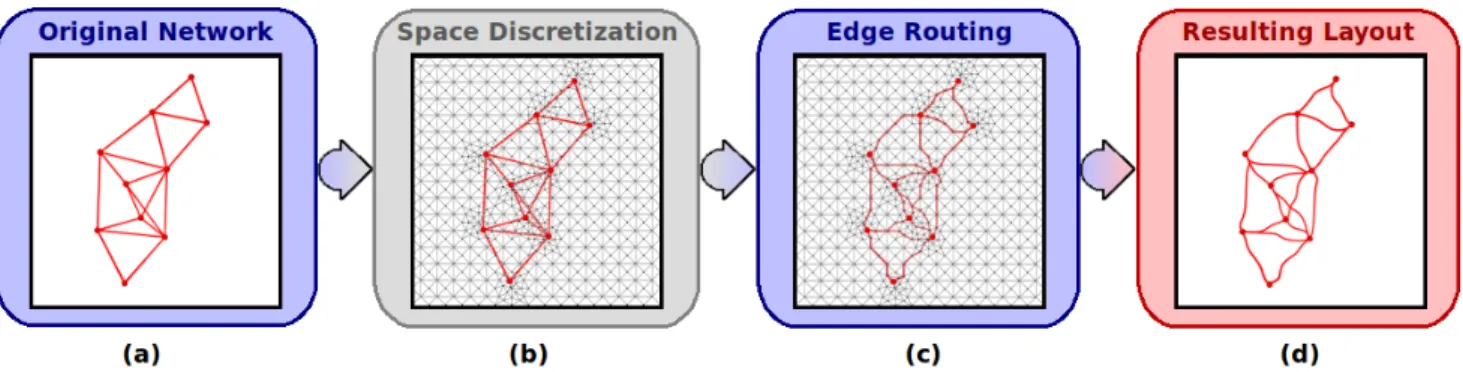
Figure 1: The main steps of our edge bundling technique. (a) Original network (here embedded in a 2D plane); (b) dis-cretization of the space; (c) Edge routing on the grid graph; (d) Resulting graph layout.
is to apply a smoothing technique on the edges drawn as polylines to morph them into curves.
Coloring edges: Another mean of enhancing
edge-bundled graph visualization is to use edges colors and opacities to encode informations. In [7], edges colors are mapped to the orientations of the original links. The same technique is used in [15] with the difference that an edge direction is encoded by an interpolated color gradient run-ning from a fixed color for the source to a fixed color for the target. In [15] edges opacities are mapped to their length, long curves being more translucent than short ones, pre-venting short curves to become obscured by long ones. In [7], the opacity of each segment of a polyline representing an edge is mapped to the density of lines overlapping it.
Perceiving bundles density: Recent work on
edge-bundled graph visualizations address the issue of estimat-ing the quantity of edges segment merged together. In [16], a GPU-based method is used to compute the amount of overdraw for each pixel of the produced graph visualiza-tion. That value is then used to map pixels colors with a user defined gradient colorscale after the minimum and maximum value of overdraw have been retrieved. A simi-lar technique is used in [18] where the overdraw densities are mapped to heights and rendered with a bump mapping technique making dense bundles appear higher than sparse ones. That technique allow users to perceive bundles den-sities while preserving edges colors.
3
Routing edges in a 3D space
3.1
Technique overview
Our technique generalized the idea presented in [18] and therefore uses an edge routing algorithm to bundle edges. Pipeline shown in figure 1 summarizes the differ-ent steps of our method. In this example, the original net-work is embedded in a 2D plane, nevertheless this figure illustrates the main idea of our technique. First of all, we discretize the space into regions according to nodes
posi-tions. Boundaries of these regions define a grid that is then used to compute the shortest routes for each edge of the original network. Like highways attract more drivers than little roads, we use frequent routes to bundle edges.
Grid computation : The first step of our method con-sists in building a grid graph used to compute the shortest routes of each original edge (i.e. edge of the original net-work). This is achieved by discretizing the space into cells or regions using nodes positions. In following, we investi-gate several approaches to create the grid graph.
Our first attempt was to build a regular 3D grid to dis-cretize the 3D space. However, using such a discretization method forces us to create really large grid graph to obtain a granularity thin enough to bundle edges even in highly dense regions of the network. To solve that problem, one can build a multi-resolution grid using for instance an oc-tree [17] or 3D Vorono¨ı diagram (for a survey on Vorono¨ı diagrams, the reader can refer to [3]). In an octree, the space is decomposed in height parts until it contains at most one element. Such approach is efficient in term of computation since its time complexity is O(|V | · log(|V |)). However, using such grid to route edges raises two main is-sues : the shortest paths computational cost (as the size of the generated grid is large), and the quality of the result (as such grid promotes horizontal and vertical routes).
In [18], Lambert et al. propose to use an hybrid algo-rithm based on both quad trees and Vorono¨ı diagrams. We follow this principle by using a combination of octree and 3D Vorono¨ı diagram.
Edge routing : The second step of the method consists in routing edges of the original graph on the grid graph built in the previous step. One can use a shortest paths al-gorithm, such as the so called Dikjstra’s algorithm [9], to achieve that operation. However, that method cannot
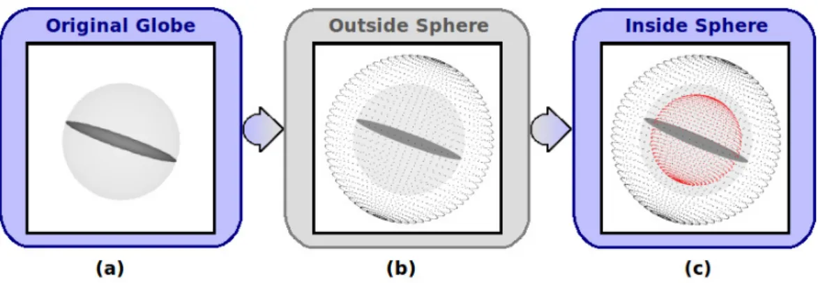
guar-Figure 2: The main preprocessing steps for bundling edges on the globe. (a) Original globe; (b) Adding dummy nodes outside the globe; (c) Adding dummy nodes inside the globe
antee that the edges will follow common routes, and there-fore, that the edges will be bundled. To create bundles, we use the metaphor of real life roads. The principle is to make attractive regular roads if highly used (i.e. if many edges are routed along these roads). We reproduce that effect by computing all the shortest paths between linked nodes of the original graph twice. During the first computation, the weight of an edge is set to the euclidean distance between its extremities. Then, according to the number of short-est paths passing through an edge of our grid, we adjust the weight of each edge. Reducing the weight of an edge is equivalent to transform it into a highway since follow-ing that edge allow to go faster from one point to another. Recomputing the shortest paths creates bundles as the new matrix distance in our graph promotes the use of highly frequent edges.
3.2
Routing edges on the globe
One of the possible applications of our method is the vi-sualization of international air interconnections in the con-text of the globe. In that case, we need to adapt our method to route edge around the globe and not across it. We thus have to guarantee that for each edge of the original net-work, there exists at least one route in the grid graph not crossing the globe. This is achieved by a preprocessing step adding dummy nodes before computing the grid graph (see figure 2). Dummy nodes are first added outside the globe in regular and spherical manner (see figure 2.(b)) to ensure that the 3D Vorono¨ı diagram will contain for each site (node of the original network) a finite cell with bound-aries (at least) partially outside the globe. However, adding these dummy nodes is not sufficient to guarantee that no edge of the grid will cross the globe. To overcome that problem we also add dummy nodes inside the globe on sphere having a smaller radius than the globe. By set-ting the radius of the internal and the external spheres of dummy nodes correctly, we can guarantee that there exists
at least one route for each original edge on the grid graph not crossing the globe.
The space discretization step of our algorithm is then applied, creating cells inside but also outside the globe. To speed up the edge routing step and to forbid routes cross-ing the globe, we remove all nodes (resp. edges) of the generated grid graph inside (resp. crossing) the globe.
3.3
Optimizations
One the main advantages of the edge routing technique to bundle edges is that some optimizations can be done to improve computation time.
As mentioned in section 3, we use the so the so called Dijkstra’s algorithm [9]. A straightforward optimization consists in not computing shortest paths between all pairs of nodes but only between each edge extremities of the original graph edge. Moreover with a slight modification of the Dijkstra algorithm, we can stop the computation of paths when all candidate nodes (in the Dijkstra’s priority queue) are at a distance greater than all the neighbors of our source node. The second optimization consists in reduc-ing the number of calls to the Dijkstra’s algorithm. More precisely, it consists in minimizing the number of nodes to treat in order to consider each edge of the graph. That prob-lem is also known as the vertex cover probprob-lem [14] and had been proved as been NP-complete. However, it is possible to compute a minimum (but not minimal) vertex cover of a graph. Finally, our method run a shortest paths algorithm for each of our vertex cover set and can therefore be paral-lelized by computing several shortest paths simultaneously. However, there are several critical sections that one needs to address. To remove some critical sections (due to the parallelization) but also generate a set of tasks with more homogeneous sizes, we use a preprocessing step that cre-ates sets of nodes that do not conflict with each other.
These improvements do not change the theoretical com-plexity but it can significantly reduce execution time.
4
Rendering bundling on the sphere
Visualizing edge-bundled graphs leverage two main is-sues. First, edges can have a quite high number of bends after the edge routing process of our technique. Conse-quently, following an edge from its source node to its tar-get node can be quite challenging when rendering edges as polylines. Second, the density of edges that have been merged into a bundle is not easily seen in the drawing. The following sections introduce the rendering techniques we applied to solve these issues.
4.1
Smoothing the edges with curves
Once the bundling process has been performed on the graph, edges become polylines due to the routing phase which adds bends to them. When rendering the edge-bundled graph layout, these bends induce a “zigzag” ef-fect on the edges making them hard to follow. In or-der to smooth edges, we offer the possibility of renor-der- render-ing them as curves in our visualization system usrender-ing edge bends as curves control points. Several kinds of parametric curves are proposed including B´ezier curves, Catmull-Rom splines and cubic B-splines. Moreover, edges going to the same region of the graph and sharing successive bends re-main merged, giving a nicer impression of flows between different areas of the graph. Due to the high computa-tional cost of rendering curves with a large number of con-trol points , especially B´ezier curves, we have developed a GPU-based implementation based on dedicated vertex
shaders. It allows us to draw a large number of curves de-fined by an arbitrary number of control points in real time, giving us the ability to smoothly interact with the graph drawing.
4.2
Edge splatting
In order to distinguish dense bundles from sparse ones, we proposed in [18] an edge splatting technique to visually enhance them. Our method is inspired from the Graph-Splatting technique introduced by van Liere et al. in [21]. In that work, the authors represent a graph as a 2D contin-uous scalar field and calculate a splat field. Our edge splat-ting rendering pipeline is based on a combination of com-mon image processing and computer graphics technique and each stage entirely runs on the GPU. In a similar way than the GraphSplatting technique, the idea is to compute a splat field encoding continuous variations in the density of merged edges. That splat field can then be displayed on screen in a various ways. We chose to render it as a height map for preserving edges colors. A per-pixel shad-ing technique is used mappshad-ing splattshad-ing values to heights giving the impression than strong bundles appears higher than weak ones. Our original edge splatting technique was restrained to graph embedded in a 2D-plane so we adapted our rendering pipeline in order to handle graph with nodes positioned on a sphere surface. The remaining summarizes
the different steps of our edge splatting rendering pipeline. The first stage of the pipeline is to compute the number of edges crossing each pixel of the drawing. As in [16], that operation can be done by performing an offscreen ren-dering of the graph edges in an accumulation buffer. Due to the fact that the graph layout is mapped on a sphere, we have to restrain the pixel overdraw computation to edges routed on the visible face of that sphere.
Next stage is the splat field computation. The resulting output of the previous stage is a field of discrete values en-coding edges density per pixel. The goal of that stage is to transform it into a continuous scalar field. That process can be performed by convoluting the discrete density val-ues field with a Gaussian kernel defined by a radius r and a standard deviation σ. The larger the kernel radius and standard deviation, the more the splat field is smoothed.
The final stage performs the splat field rendering using a classical shading technique called bump mapping. Bump mapping is a computer graphics technique introduced by Blinn [6] allowing a rendered surface to appear more real-istic without modifying geometry. It adds a per-pixel shad-ing that makes the surface appears bumpy, by changshad-ing the surface normals. These modified normals are computed from a heightmap generated by mapping the splatting val-ues to a black to white color scale. A dedicated fragment
shadercompute for each pixel the heightmap derivatives in horizontal and vertical directions using a gradient operator, like the Sobel or Prewitt filter, and construct the associated normals from these. Once the normal map associated with the splat field has been generated, bump mapped render-ing can be performed. Because we want to perform bump mapping on a sphere surface and not on a flat one, we add an extra process to our original pipeline. Its goal is to com-pute for each pixel of the sphere’s visible face the transfor-mation of the light vector and the eye vectors into tangent
space. That space is locally tangent to the surface and is used to compute the final colors of the pixels in a bump mapping context. That process is performed by rendering a sphere in an offscreen buffer, whose center and radius are the same as the graph layout, with tangent space infor-mations attached to each vertex of the mesh. A dedicated
shader programthen transforms the light and eye vectors provided as parameters into tangent space and stores the re-sults in two floating point textures. The final bump mapped drawing is then generated by another shader program read-ing the modified normals from the normal map texture, the transformed light and eye vectors from the two previous generated textures, and performing a per-pixel illumination using Blinn-Phong [5]. The final colors of the pixels are computed from the lighting properties and another texture called the diffuse map. In our case, the diffuse map corre-sponds to the original edge colors. To perform a global
il-(a) (b) (c)
(d) (e) (f)
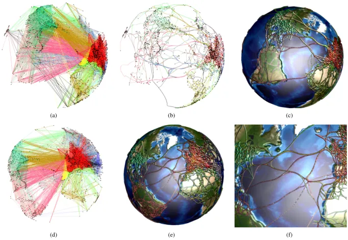
Figure 3: (a) 2000 international air interconnections network, containing 1524 airports and 16397 flights, embedded on the globe; (b) Result when applying the 3D edge routing method and using spline curves;(c) Result when routing edge around the globe and using cubic b-spline curves and bump mapping ; (d) 2004 international air interconnections network, containing1501 airports and 12360 flights, embedded on the globe ;(e) Result when applying the 3D edge routing method and using cubic b-spline curves and bump mapping ; (f) Zoomed view.
lumination, the light is set to be directional with each light ray parallel to the Z-axis. Our visualization system then lets the user configure the ambient, diffuse and specular color of the light source. The view can also be zoomed, panned and rotated for interactive exploration.
5
Results
We experimented our algorithm on the international air interconnection networks of year 2000 and year 2004 (see figure 3). Figures 3.(a) and (d) show the original layout of both air traffic networks when nodes are laid out ac-cording to their latitudes and longitudes. An edge color is computed according to the geographical regions its ex-tremities belong to (for instance, european flight are repre-sented by red edges while north american ones are in dark green). These representations are difficult to understand due to the visual complexity of such networks and to
oc-clusion problems raised by 3D visualization. Using our 3D edge bundling technique (see figure 3.(b)) reduces the clutter of the representation. One can already see some of the major trends, such as really dense intra european and north american networks. However as the number of pos-sible routes for each original edge is large, edges are not bundled enough and the representation still suffers from occlusion problems.
Figures 3.(c) and .(e) show the result we obtained when routing the edges around the globe and not across it. To in-crease the readability of that drawing, we added a texture to render the continents and seas. These drawings had been computed in90 seconds for the 2000 air traffic network and84 seconds for the 2004 air traffic network 1. When looking closer to the results one can notice that edges col-ors in each bundle are more or less uniform, meaning that
edges bundled together are linking the same geographical regions. For instance, figure 3.(f) is a zoomed view on the 2004 air traffic network, one can see that all edges between Europe and North America were bundled together in the light brown bundles. In these figures, one can see major trends, such as the central positioning of Europe within both networks or that Africa is mainly related to european and middle east countries. Our technique clearly improves the readability of these representations and help to reveal high-level edge patterns.
Conclusions
In this paper, we have presented A 3D edge bundling technique based on edge routing. This technique allows to reduce clutter of a 3D representation but also reveals high-level edge patterns. We have also introduced the needed modifications to bundle the edges on the sphere in or-der support visualization geographical networks, such as the international air traffic networks, in the context of the globe.
To facilitate edge bundle density perception, we pre-sented a GPU-based rendering method that allows a fast enough rendering to support smooth exploration. That method is an extension of the bump-mapping technique of [18] which allows to preserve edge colors in order to encode another information.
An interesting direction for future work is to explore different methods to build the grid graph such as a grid sup-porting non-uniform nodes sizes or avoiding regions of the representation. Another direction is to adapt our method to surfaces having other topologies. Finally we plan to speed up the rendering by minimizing the number of bends. This bends simplification should also guarantee that no node-edge overlap is created.
References
[1] J. Abello, F. van Ham, and N. Krishnan. ASK-GraphView : A Large Graph Visualisation System.
IEEE Transactions on Visualization and Computer Graphics, 12(5):669–676, 2006.
[2] D. Archambault, T. Munzner, and D. Auber. Grouse: Feature-Based and Steerable Graph Hierarchy Explo-ration. In Ken Museth, Torsten M¨oller, and Anders Ynnerman, editors, Eurographics/ IEEE-VGTC
Sym-posium on Visualization, pages 67–74, Norrk¨oping, Sweden, 2007. Eurographics Association.
[3] F. Aurenhammer. Voronoi diagrams—a survey of a fundamental geometric data structure. ACM Comput.
Surv., 23(3):345–405, 1991.
[4] M. Balzer and O. Deussen. Level-of-detail visualiza-tion of clustered graph layouts. In Asia-Pacific
Sym-posium on Visualization, pages 133–140, 2007.
[5] James F. Blinn. Models of light reflection for com-puter synthesized pictures. In SIGGRAPH ’77:
Pro-ceedings of the 4th annual conference on Computer graphics and interactive techniques, pages 192–198, New York, NY, USA, 1977. ACM.
[6] James F. Blinn. Simulation of wrinkled surfaces. In
SIGGRAPH ’78: Proceedings of the 5th annual con-ference on Computer graphics and interactive tech-niques, pages 286–292, New York, NY, USA, 1978. ACM.
[7] W. Cui, H. Zhou, H. Qu, P. C. Wong, and X. Li. Geometry-based edge clustering for graph visualiza-tion. IEEE Transactions on Visualization and
Com-puter Graphics, 14(6):1277–1284, 2008.
[8] M. Dickerson, D. Eppstein, M. T. Goodrich, and J. Y. Meng. Confluent Drawings: Visualizing Non-planar Diagrams in a Planar Way. In Proc. Graph Drawing
2003 (GD’03), pages 1–12, 2003.
[9] E. W. Dijkstra. A short introduction to the art of
programming. Technische Hogeschool Eindhoven, 1971.
[10] D.P Dobkin, E.R. Gansner, E. Koutsofios, and S.C. North. Implementing a general-purpose edge router. In Proc. Graph Drawing 1997 (GD’97), pages 262– 271, 1998.
[11] T. Dwyer and L. Nachmanson. Fast Edge-Routing for Large Graphs. In Proc. Graph Drawing 2009
(GD’09), page To appear, 2010.
[12] G. Ellis and A. Dix. A taxonomy of clutter reduction for information visualisation. IEEE Transactions on
Visualization and Computer Graphics, 13(6):1216– 1223, 2007.
[13] E. R. Gansner and Y. Koren. Improved circular lay-outs. In Proc. Graph Drawing 2006 (GD’06), pages 386–398, 2006.
[14] D. S. Hochbaum. Approximating covering and pack-ing problems: set cover, vertex cover, independent set, and related problems. pages 94–143, 1997. [15] D. Holten. Hierachical Edge Bundles: Visualization
of Adjacency Relations in Hierarchical Data. IEEE
Transactions on Visualization and Computer Graph-ics, 12(5):805–812, 2006.
[16] D. Holten and J. J. van Wijk. Force-directed edge bundling for graph visualization. In 11th
Eurographics/IEEE-VGTC Symposium on Visualiza-tion (Computer Graphics Forum; Proceedings of Eu-roVis 2009), volume 31, pages 983–990, 2009.
[17] C. L. Jackins and S. L. Tanimoto. Oct-trees and their use in representing three-dimensional objects.
Com-puter Graphics and Image Processing, 14(3):249– 270, 1980.
[18] A. Lambert, R. Bourqui, and D. Auber. Wind-ing roads: RoutWind-ing edges into bundles. In 12th
Eurographics/IEEE-VGTC Symposium on Visualiza-tion (Computer Graphics Forum; Proceedings of Eu-roVis 2009). To appear., 2010.
[19] D. Phan, L. Xiao, R. Yeh, P. Hanrahan, and T. Wino-grad. Flow map layout. In Proc. of IEEE Information
Visualization Symposium, pages 219–224, Washing-ton, DC, USA, 2005. IEEE Computer Society. [20] F. van Ham and J. J. van Wijk. Interactive
Visual-ization of Small World Graphs. In Proc. of IEEE
In-formation Visualization Symposium, pages 199–206, Washington, DC, USA, 2004. IEEE Computer Soci-ety.
[21] R. van Liere and W. de Leeuw. GraphSplatting: Vi-sualizing graphs as continuous fields. IEEE
Trans-actions on Visualization and Computer Graphics, 9(2):206–212, 2003.
[22] N. Wong and S. Carpendale. Using Edge Plucking for Interactive Graph Exploration. In Proc. of IEEE
Information Visualization Symposium, Poster Com-pendium, pages 51–52, Washington, DC, USA, 2005. IEEE Computer Society.
[23] N. Wong, S. Carpendale, and S. Greenberg. Edge-Lens: An Interactive Method for Managing Edge Congestion in Graphs. In Proc. of IEEE Information
Visualization Symposium, pages 51–58, Washington, DC, USA, 2003. IEEE Computer Society.
[24] M. Wybrow, K. Marriott, and P.J. Stuckey. Incremen-tal connector routing. In Proc. Graph Drawing 2005
(GD’05), pages 446–457, 2006.
[25] H. Zhou, X. Yuan, W. Cui, H. Qu, and B. Chen. Energy-based hierarchical edge clustering of graphs. In Visualization Symposium, 2008. PacificVIS ’08.