Cognitive Information Processing

XX. COGNITIVE INFORMATION PROCESSING

Academic and Research Staff

Prof. S. J. Mason Prof. B. Prasada Dr. P. A. Kolers Prof. W. L. Black Prof. O. J. Tretiak Dr. N. Sezaki Prof. M. Eden Prof. D. E. Troxel K. R. Ingham Prof. T. S. Huang Prof. D. Cohen G. L. Wickelgren

Dr. M. P. Beddoes Graduate Students

A. K. Bhushan P. H. Hartmann J. A. Newell J. D. Bigham, Jr. M. Kawanami L. C. Ng

D. Caldwell E. E. Landsman D. H. Pruslin

A. L. Citron M. B. Lazarus C. L. Seitz

R. W. Cornew F. F. Lee S. D. Shoap

A. Gabrielian J-H. Liu A. Spiridon

B. P. Golden J. I. Makhoul J. A. Williams

A. COGNITIVE PROCESSES

1. AN ILLUSION THAT DISSOCIATES MOTION, OBJECT, AND MEANING

If one looks for a minute at a simple Archimedes (arithmetic) spiral that is rotating approximately 2-3 times per second, and then looks at something else, the second object will appear to change size and sometimes distance also. The direction of change in the second object is exactly opposite to that of the spiral: if the spiral rotates "inward," the aftereffect is an expansion of visual objects; and if the spiral rotates "outward," the aftereffect is a contraction. By "inward" we mean clockwise in the spiral of Fig. XX-1. It is sometimes assumed that this illusory motion of the spiral is based on the same mechanism as that for the usual illusion of visual appar-ent motion, or "phi motion," as it is some-times called. This assumption is probably wrong; the two illusions seem to have dif-ferent mechanisms. We shall describe a new illusion that seems to dissociate the motion aspects of the spiral aftereffect from the location of objects in space and, in turn, from the interpretation of those objects. Fig. XX-1. Spiral of Archimedes. Let a target be prepared that consists of

*This work was supported in part by the Joint Services Electronics Programs (U. S. Army, U.S. Navy, and U. S. Air Force) under Contract DA 36-039-AMC-03200(E), and in part by the National Science Foundation (Grant GK-835), the National Institutes of Health (Grant 2 PO1 MH-04737-06), and the National Aeronautics and Space Administra-tion (Grant NsG-496).

a regular matrix of crossing lines (Fig. XX-2), the whole target subtending, say, 200 of visual angle on each side, and the squares within it occupying approximately 0. 50

each. A subject who looks at this matrix will report it as regular and with all the

squares apparently of the same size (as in fact they are drawn.) He tends to see some lightening and darkening in the areas in which the vertical and horizon-tal lines cross, but this is eliminated if he is not permitted to look too long

(more than a few seconds) at the matrix. Now let the subject look at a spiral whose diameter is 40 visual angle. As it rotates "inward" a number of curious and Fig. XX-2. Square matrix. interesting visual distortions occur in its shape and color. Typically, there is some lightening of the black regions and darkening of the white; all subjects see the motion of the spiral; and the larger number of them report a change in the apparent depth of the figure: the spiral takes on the appearance of a three-dimensional coil, the inner-most part appearing inner-most distant (or nearest when the rotation is outward"). These

apparent changes have been noted many times in the past hundred years, but still are not satisfactorily explained; so we proceed, having acknowledged their existence, to the main observations.

After looking at the spiral for a minute, let the subject transfer his gaze to a single square of the large matrix, one near its center. He then reports that many of the small cells (Fig. XX-2) change size drastically; for example, by a factor of 10-20. Not all of the cells change size; rather, only those change that occupy a region of the matrix that corresponds in angular subtense to the region previously

stimu-lated by the spiral. That is to say, if the spiral had occupied approximately 40 visual angle, the cells of the matrix that fall within a diameter of 40 centered on the square chosen for fixation are the ones that subsequently appear to change in size. Many subjects also report that the apparent distance of the cells also changes. In fact, then, what is usually reported is that a small region of the large matrix changes in size and

apparent distance as a result of looking at the spiral. This itself is to be expected from what was said above. What is not expected is that simultaneously with a change in the

apparent size and distance of some of the cells, no discontinuity with the remainder appears. The illusion therefore consists in the logically impossible situation that part of a two-dimensional array changes size and distance without undergoing any discontinuity

(XX. COGNITIVE INFORMATION PROCESSING)

in the lines that join it to the remainder of the figure. How can this be explained? Let it be assumed that there are at least three distinguishably different "systems" in the visual nervous apparatus: one system is concerned with the perception of contours;

a second with the perception of motion; and the third with interpretation or "meaning." We have shown previously that the usual form of illusory motion (the stroboscopic motion created by motion pictures or television) actually seems to have little to do with the actual processing of motion; rather, that effect seems to be due to a perceptual

filling-in or impletion between the successive locations of a discontinuously displaced object. 1 That motion is truly illusory in that it is imposed on the output of the contour-perception system, and not of any motion-detection system. With the rotating spiral,

on the other hand, the visual apparatus is actually stimulated by a truly moving figure. The changes in visual objects that are seen after looking at the rotating spiral must be interpretations imposed on the motion-detection system. This belief is supported by the fact that sustained observation of stroboscopic motion (an impletion from the

contour-detection system) does not yield any of the changes in figure properties of a subsequently looked-at target that occur after looking at a rotating spiral. Thus we believe that a unique motion-detection system is activated by the rotating spiral, and a contour-detection system by stroboscopic motion. The failure to observe discontinuities in the large matrix results from the fact that such discontinuities, if they existed, would be detected by the contour-detection system, not by the motion system. Furthermore, the recognition of the logical paradox of the absence of discontinuities must be due to still another system, which is concerned with interpretation or "meaning" at a higher level than object recognition. It might also be pointed out that unlike the case with many

per-ceptual illusions whose paradoxial nature causes some discomfort or annoyance, there is no such sense present with this illusion. In fact, most observers (and we have tested

50) usually fail to note the paradox until it is pointed out. Still, the precise mechanisms that mediate the interaction of the motion and object-detection systems have still to be worked out, as have the rules that govern the formation of impletions.

P. A. Kolers References

1. P. A. Kolers, "The Illusion of Movement," Scientific American 211, 98-106 (1964).

B. PICTURE PROCESSING 1. OPTIMUM BINARY CODE Introduction

Some progress has been made on the problem of optimum binary code as discussed in previous reports1, ' 2: (a) Conjectures 2 and 3 of an earlier report2 have been proved

to be true; and (b) A computer simulation has been carried out for the special case of 3-bit codes. These will be described briefly here. Also, a general expression has been derived for the mean-absolute error of the natural code, which is reported in Sec-tion XX-B. 2.

Average Noise Power of Reflected-Binary Gray Code

A general expression was derived for the average noise power (i. e., mean-square error) of the reflected-binary Gray code.3 We state this result as

THEOREM 1. Consider the transmission of integers over a BSC, using fixed-length binary block codes. If the input data are uniformly distributed over the integers 0 to 2n - 1, then the mean-square error for the reflected-binary Gray code is

1 - 2p 4 - (l-2p)n

G _n -₆ (4 -) _{2 4 - (1-2p) '} (1)

where p is the probability of error of the BSC.

After some manipulations, we have, from Eq. 1 and Eq. 1 of our previous report,l the following theorems.

THEOREM 2. Under the same assumptions as in Theorem 1, we have

(Gn-Nn) = (1-2p)Gn_-, ₍₂₎

where Nn is the mean-square error of the n-bit natural code.

THEOREM 3. Under the same assumption as in Theorem 1, and assuming further 1

that p <- , we have

N G (3)

n n

That is, the natural code yields a smaller mean-square error than the reflected-binary Gray code.

Computer Simulation of 3-bit Codes

A computer program has been written4 and run, which calculated the mean-square and the mean-absolute errors of all possible 3-bit codes and gave the results as poly-nomials in p, the error probability of the BSC.

It was found that the natural code yields both the minimum mean-square error and 1

the minimum mean-absolute error, for p -2. The reflected-binary Gray code has the same mean-absolute error as the natural code, but has a larger mean-square error than

1 the natural code for p < 2.

T. S. Huang

(XX. COGNITIVE INFORMATION PROCESSING)

References

1. Y. Yamaguchi and T. S. Huang, "Optimum Binary Fixed-Length Block Codes," Quarterly Progress Report No. 78, Research Laboratory of Electronics, M. I. T., July 15, 1965, pp. 231-233.

2. Y. Yamaguchi and T. S. Huang, "Optimum Binary Code," Quarterly Progress Report No. 79, Research Laboratory of Electronics, M.I.T., October 15, 1965, pp. 214-217.

3. K. A. Achterkirchen, Course 6. 39 Term Project Report, Department of Electrical Engineering, M.I.T., May 20, 1966.

4. T. F. Strand, S. B. Thesis, Department of Electrical Engineering, June 1966.

2. ERROR IN FIXED-LENGTH NONREDUNDANT CODES

Let us assume that we have 2n equiprobable signals with values 0, 1, 2, ... Zn-1 and we wish to code these in terms of binary n-tuples, to be transmitted through a binary symmetric channel.

Harper1 has proved the following theorem.

THEOREM. To obtain a code that minimizes the average absolute error when only one error per signal is considered, assign zero to an arbitrary vertex of the binary n-cube, and, having assigned 0, 1, 2, . . .,, assign 2 + 1 to an unnumbered vertex (not necessarily unique) which has the most numbered nearest neighbors.

The value of this minimum average error is (2n-1) p(l-p)n - 1 which is quite easy to compute.

We shall derive an expression for the absolute error of the "Harper codes" when all possible combinations of errors are allowed.

Define an equivalence relationship such that two possible coding schemes are in the same equivalence class if and only if they give the same mean absolute error for all values of p.

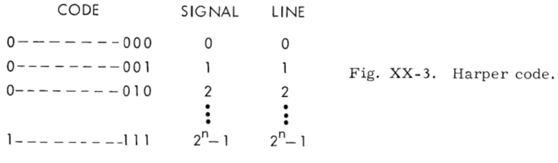
THEOREM. The codes obtained by the Harper scheme form an equivalence class. The details of the proof will be omitted, but it hinges on the fact that in a serial listing of a Harper code corresponding to the signals 0, 1, . .. 2n - 1 (see Fig. XX-3) if the group of codes on lines £1= 0 mod fo through £1 + - 1; 0 < 0< 2n; 0 _ 1 2n - 2 are flipped around their mid-point, the average error for any particular combi-nation of errors does not change. These flipping operations generate all of the Harper codes starting from any particular one, if we consider the different permutations pos-sible on the columns of the codes.

It is conjectured that the above-mentioned class has the least average absolute error, but we have not been able to prove this yet.

THEOREM. The average absolute error for the class of codes obtained by the Harper scheme is p(2n-(l-p)n)/(l+p).

Proof: We shall prove this _{by calculating the average absolute error for a specific} member of the class of codes obtained by the Harper scheme, namely the so-called

"natural code" that assigns to each number its binary representation.

CODE

SIGNAL

LINE

0---000

0___ -

-- -- 001

I

0---001

0---01

0

I_----111

Consider the occurrence of

binary representation is at the

0

2

2n

1

Fig. XX-3. Harper code.

2n

k errors in the codes such that the leftmost error in the mth bit from the right. For each signal there are _{ar k-1 J} m-such possible errors. We note that for any signal I with binary representation

nxn-1 ... Xm+l

lXm-l

I'

x

m m-1

X X

m2 m2 -1 mk-I mk-1-1

(-1) 2 . - (-I) 2 . For this same combination of errors in

I'

x

_{m1 2m-}

x

1

mk-1

k

absolute error in ' is 2 + (-1) 2 +... + (-1) 2 The proba-bility of occurrence of such an error is (-p) n - k

pk for both f and ', and these two are assumed to be equiprobable themselves. _{It follows that the average absolute error for} any k error with leftmost error at bit m is 2 m - _,

as all of the other terms cancel out in computing the average over the ensemble.

- n

The average absolute error is E = pm I

E

m= 1

the leftmost error is on bit m, and CmE _{is the average absolute error with leftmost}

error on bit m. Now we have just shown that m= 2m - and p is (1-p)n p so

n = (l-p)n - m p2 m= 1 = p(i-p)n 2 aPR No. 82 n (2/(l-p))m m= l 226

(XX. COGNITIVE INFORMATION PROCESSING)

1E = p(l-p)n (2/(1-p))n+

_

(2/(1-p))-

1

= p(2n-(1-p)n)/(l+p)

Q. E. D. Calculation of the number of equivalence classes and, in fact, a complete classifica-tion of them in terms of their associated errors appear to be within the realm of possi-bility and will form part of the further investigation of this problem.

A. Gabrielian, T. S. Huang

References

1. H. Harper, "Optimal Assignment of Numbers to Vertices," J. Soc. Indust. Appl. Math., Vol. 12, No. 1, 1964.

3. EFFECT OF BSC ON PCM PICTURE QUALITY Introduction

The current trends in communication point in the direction of PCM.1 In particular, the transmission of pictures by PCM has attracted wide attention.2 In order to design a PCM picture-transmission system efficiently, it is desirable to collect data on the effects of system parameters on received picture quality.

An important factor in a communication system is the channel noise. The subjec-tive effects of noise in analog picture-transmission systems have been studied

exten-sively.3 - 8 No data are available, however, on digital systems. For binary PCM transmission systems, a first approximation to many practical channels is the binary symmetric channel (BSC) without memory. The error probability, p, of the BSC is a parameter which can be traded off with other system parameters such as the energy per bit of the signal.

The purpose of the present report is to give some results on the subjective effect of the noise introduced in the received pictures of a PCM system by the BSC. Specif-ically, such noise was compared, with regard to its subjective effect, with noise intro-duced by an additive white Gaussian channel to a PAM transmission system. The latter was chosen as a standard because its appearance is similar to that of the familar "snow" that is observed on a home television screen. It was assumed that the pictures were of a general nature, and were transmitted for the purpose of entertainment.

The two systems were simulated on an IBM 7094 computer to produce noisy pictures. Subjective tests were then carried out to compare the objectionability of the two types

of noise. Three original pictures, varying in the amount of details, were used. It was found true of all three pictures that for high signal-to-noise ratios the white Gaussian noise is more objectionable than the BSC noise, while for low signal-to-noise ratios the

reverse is true. The crossover point lies approximately in the range 16-20 db peak signal-to-rms-noise ratio, and tends to occur at a higher signal-to-noise ratio for a picture having more details. The noise used in the signal-to-noise ratio calculation was the difference between the brightness of the received picture and that of the transmitted

picture.

Generation of Noisy Pictures

The noisy pictures were generated on an IBM 7094 digital computer.

a. Digitalization of Pictures

A digital scanner 9 was used to sample and quantize pictures and to record the digit-alized data on magnetic tape in a format compatible with the IBM 7094 computer. For the present study, 256 X 256 samples were taken of each picture, and the brightness of

(XX. COGNITIVE INFORMATION PROCESSING)

each sample was quantized to 128 levels, or 7 bits.

The magnetic tape was used as input

for computer processing. The processed picture was written on an output magnetic tape

by the computer.

The digital scanner was again used to display the processed picture

from the output magnetic tape on a cathode-ray tube, from which a hard copy of the

picture was taken.

b.

PAM Picture Transmission through an Additive White Gaussian Channel

Independent Gaussian random variates with mean zero and variance one were

gen-erated, and then the received picture r(x, y) was obtained from the transmitted picture

s(x, y) by the following equation:

r(x, y)

=

s(x,y) + n(x,y)

s(x, y) + rnl (x, y),

(1)

where x and y are the spatial coordinates of a picture sample, and nl(x,y)

=

Gaussian

random variates with mean zero and variance one, independent from sample to sample,

and independent of S(X, Y).

The peak signal-to-rms noise of the received picture r(x, y)

then is

N)db = 20 log

,

(2)

where A is the peak signal value.

In our case, A

=

127.

c.

PCM Picture Transmission through a BSC

We assumed that a straight binary code was used for the brightness levels of the

picture.

The binary symmetrical channel (with error probability 0 -- p

<

1) was

sim-ulated as follows.

For each signal bit, an independent random variate with uniform

dis-tribution (over the unit interval [0, 1] was generated.

The received bit was set to be the

same as or different from the transmitted bit, according as this random variate was

greater than p, or was less than or equal to p.

Again, we use s(x, y) to denote the transmitted picture, and r(x, y), the received one.

The noise is defined as

n(x, y) = r(x,y) - s(x,y) (3)

Young and Mott-Smithl0 have shown that, under certain conditions (in particular, if the

probability distribution of the brightness levels in the picture s(x, y) is flat, or if it is

symmetrical with respect to the mean), the noise power n2 is related to the error

prob-ability by

B

2

4

where B is the number of bits in each code word. In our case, B = 7. The probability distributions of the pictures used in our study did not exactly satisfy the conditions for the validity of Eq. 4; however, actual computer calculations of nZ yielded results that fitted Eq. 4 almost perfectly.

d. Pictures Generated for This Study

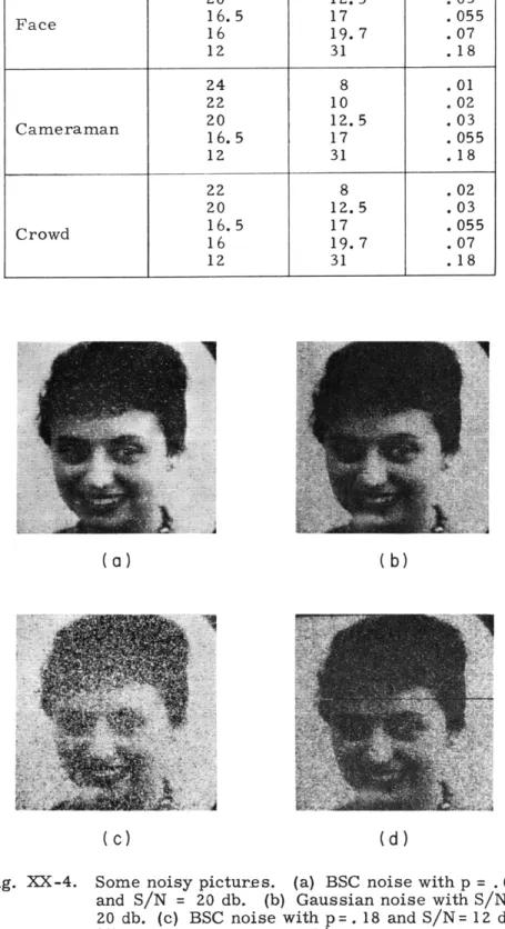
Three original pictures were used: a face of a girl, a scene with a cameraman as a central object, and a crowd. Four signal-to-noise ratios were used for the face, and five each for the cameraman and the crowd. For each original picture and each signal-to-noise ratio, two noisy pictures were generated: one containing white Gaussian noise and the other BSC noise, resulting in eight noisy pictures for the face, and ten noisy pictures each for the cameraman and the crowd. The signal-to-noise ratios used are listed in Table XX-1. Some of the noisy pictures are shown in Fig. XX-4.

Subjective Tests and Results

Two types of subjective tests were carried out: paired comparison, and matching. In all tests, hard copies of the pictures were shown to the observers, and the viewing

distance was 15 inches, which is six times the picture height. The size of the pictures was 2. 5 in. X 2. 5 in.

a. Paired Comparison Tests

The objective of these tests was to find out, for a given signal-to-noise ratio, which of the two types of noise, Gaussian or BSC, was more objectionable to human observers.

Each observer was shown two noisy pictures at a time. These two pictures had the same subject matter and the same signal-to-noise ratio, but one picture had Gaussian noise and the other, BSC noise. The observer was asked to choose the picture he pre-ferred to watch, say, on a television screen. Forty observers took the tests with the picture of the cameraman. For the pictures of the face and the crowd, there were 15 observers.

The results of these tests are given in Table XX-2. The number corresponding to (i. e. , at the intersection of) a particular noise type and a particular S/N represents the total number of observers who preferred that noise type to the other type at that S/N. For example, 21 observers preferred BSC noise to Gaussian noise at an S/N of 24, for the picture of the cameraman.

b. Matching Tests

The objective of these tests was to find out, for two pictures with the same subject matter but different types of noise (Gaussian noise in one, and BSC noise in the other) to be equally objectionable to human observers, what should be the relation between their

Table XX- 1. Peak signal-to-rms noise ratios, S/N, used in

this study, with the corresponding rms noise,

a, and the error probability of the BCS, p.

(a)

(b)

(c)

(d)

Fig. XX-4.

Some noisy pictures.

(a) BSC noise with p

= .03

and S/N

=

20 db.

(b) Gaussian noise with S/N

=

20 db. (c) BSC noise with p=. 18 and S/N= 12 db.

(d) Gaussian noise with S/N = 12 db.

()N db P 20 12.5 .03 16.5 17 .055 16 _19.7 .07 12 31 .18 24 8 .01 22 10 .02 20 12.5 .03 16.5 17 .055 12 31 .18 22 8 .02 20 12.5 .03 16.5 17 .055 16 19.7 .07 12 31 .18

(a) Face

(b) Cameraman

(c) Crowd

Total number of preferences for picture with various (S/N)db Type of noise 22 20 16.5 16 12 BSC 11 13 6 4 0 Gaussian 4 2 9 11 15

QPR No. 82

Total number of preferences for picture with various (S/N)db Type of noise

20 16.5 16 12

BSC 13 8 4 0

Gaussian 2 7 11 15

Table XX-3. Results of matching tests.

(a) Face

(b) Cameraman

Rank for picture with various (S/N)db

24

22

20

16.5

12

BSC

1

2

3

4

5

Gaussian

1.7

2.5

3. 2

3. 7

4.5

(c) Crowd

Rank for picture with various (S/N)db

22

20

16.5

16

12

BSC

1

2

3

4

5

signal-to-noise ratios.

The pictures with BSC noise were ordered according to their signal-to-noise ratios. The picture with the highest S/N was given rank 1, the picture with the second highest S/N was given rank 2, and so forth. This set of pictures was put in front of the observer. He was then shown a picture chosen at random from the set of pictures with Gaussian noise, and asked to match it, according to noise objectionability, with the set of pictures with BSC noise. The Gaussian picture was assigned a rank equal to that of the BSC picture to which it was matched. If the Gaussian picture was rated between two BSC pictures, it was given a rank equal to the average of the ranks of the two BSC pictures.

Thirty-five observers were tested for the picture of the cameraman, and 15 for the pictures of the face and the crowd. The ranks of the Gaussian pictures averaged over all observers are given in Table XX-3.

Evaluation of Data a. General Trends

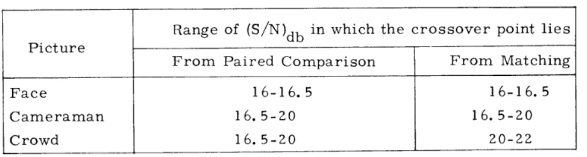
From Tables XX-2 and XX-3, we see that for high signal-to-noise ratios, more observers preferred BSC noise to Gaussian noise, while the reverse was true for low signal-to-noise ratios. The ranges in which the crossover points lie can be obtained from either Table XX-2 or Table XX-3. They are listed in Table XX-4.

Table XX-4. Crossover points.

Range of (S/N)db in which the crossover point lies

Picture

From Paired Comparison From Matching

Face 16-16.5 16-16.5

Cameraman 16. 5-20 16. 5-20

Crowd 16. 5-20 20-22

We see that the results from the two methods agree with each other except in the case of the crowd. Even in that case, however, inspection of Table XX-3(c) reveals that the crossover point according to the matching tests is very close to 20 db. The data of Table XX-4 indicate that as the amount of detail in a picture increases, the crossover point moves to a higher signal-to-noise ratio.

The general trends discussed here may probably be explained in the following man-ner. It is evident from Fig. XX-4 that the Gaussian noise degrades the entire picture

(XX. COGNITIVE INFORMATION PROCESSING)

uniformly and creates a blurring effect, while the BSC noise appears to consist of iso-lated white and black dots. At a high signal-to-noise ratio these dots, since they are scattered over the picture, do not obscure any picture details; but when the signal-to-noise ratio decreases, the density of the dots becomes large, and details in the picture

begin to be obscured, and therefore the BSC noise becomes very objectionable.

25 - _{Also, at a given signal-to-noise ratio,}

more details would tend to be obscured

20 -/ by the dots (and therefore the noise would

appear more objectionable) in a picture

5 / with a large amount of detail such as

u fthe crowd picture, than in a picture with

'u

S/ a small amount of detail such as a face 3 O 10

-0o / picture.

0 5 10 15 20 25

PEAK SIGNAL-TO-RMS NOISE RATIO OF GAUSSIAN PICTURE (db)

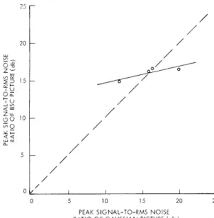
Fig. XX-5.

b. Isopreference Curves

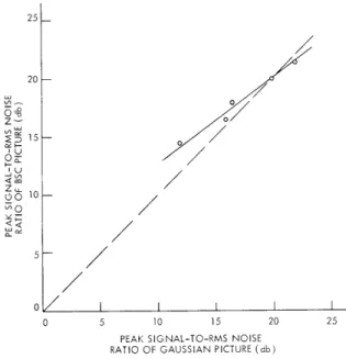
Isopreference curves (i. e. , curves expressing the relation that the signal-to-noise ratios of Gaussian and BSC pic-tures must satisfy for the two picpic-tures to be equally preferable) were obtained from Table XX-3. This was done by estimating the signal-to-noise ratios of BSC pictures corresponding to the ranks of the Gaussian pictures listed in Table XX-3. If a rank m satisfied

k<m <k+ 1,

where k was an integer, and if the signal-to-noise ratios of BSC pictures corre-sponding to ranks k and k + 1 were a and b, then, c, the signal-to-noise ratio of the BSC picture corresponding to rank m

was estimated as

0 / I I I I I

0 5 10 15 20 25

PEAK SIGNAL-TO-RMS NOISE RATIO OF GAUSSIAN PICTURE (db)

Fig. XX-6. Isopreference curve for the

picture of the cameraman.

c = a - (m-k)(a-b).

The isopreference curves for the three original pictures are plotted in Figs. XX-5, XX-6, and XX-7. The solid

20 S15 U cc Z 1 ,

25 20 D 15 Z' 0 0 5 0 I I I I 0 5 10 15 20 25

PEAK SIGNAL-TO-RMS NOISE RATIO OF GAUSSIAN PICTURE (db)

Fig. XX-7. Isopreference curve for the picture of the crowd.

lines are the linear least-mean-square fit to the data points. The dotted lines are the lines with unit slope on which the Gaussian and BSC pictures have the same signal-to-noise ratios. These plots express in a quantitative way the general trends that we have discussed.

T. S. Huang, M. T. Chikhaoui

References

1. E. M. Deloraine and A. H. Reeves, "The 25th Anniversary of Pulse Code Modu-lation," IEEE Spectrum, Vol. 2, No. 5, pp. 56-63, May 1965.

2. T. S. Huang, "PCM Picture Transmission," IEEE Spectrum, Vol. 2, No. 12, pp. 57-63, December 1965.

3. J. M. Barstow and H. N. Christopher, "The Measurement of Random Monochrome Video Interference," Trans. AIEE, Vol. 73, Part 1, pp. 735-741, January 1954. 4. J. M. Barstow and H. N. Christopher, "The Measurement of Random Video

Inter-ference to Monochrome and Color Television Pictures," Trans. AIEE, Communica-tions and Electronics, Vol. 63, pp. 313-320, November 1962.

5. R. C. Brainard, F. N. Kammerer, and E. G. Kimme, "Estimation of the Subjective Effects of Noise in Low-Resolution Television Systems," IRE Trans., Vol. IT-8, No. 2, pp. 99-106, February 1962.

6. T. S. Huang, "The Subjective Effect of Two-Dimensional Pictorial Noise," IEEE Trans., Vol. IT-11, No. 1, pp. 43-53, January 1965.

7. P. Mertz, "Perception of Television Random Noise," J. SMPTE, Vol. 54, pp. 8-34, January 1950.

8. P. Mertz, "Data on Random-Noise Requirements for Theater Television," J. SMPTE, Vol. 57, pp. 89-107, August 1951.

(XX. COGNITIVE INFORMATION PROCESSING)

9. T. S. Huang and O. J. Tretiak, "Research in Picture Processing," in Optical and Electro-Optical Information Processing, edited by J. Tippet, et al. (The M. I. T. Press, Cambridge, Mass. , 1965).

10. I. T. Young and J. Mott-Smith, "On Weighted PCM," IEEE Trans., Vol. IT-11, No. 4, pp. 596-597, October 1965.

C. PATTERN-RECOGNITION STUDIES

1. COMPUTER SIMULATION OF BIOLOGICAL PATTERN GENERATION: A PRELIMINARY REPORT

Introduction

A complete survey of the field will not be attempted here. Rather, reference is made to the excellent book by C. H. Waddington1 which discusses in some detail the problems of biological pattern generation, or morphogenesis, and its relation to genetic information.

Several lines of evidence suggest that although the DNA base sequence in the genome may only be specifying a particular sequence of bases in RNA molecules, and through it a collection of amino-acid sequences in proteins, the over-all pattern of development and morphogenesis is the result of a hierarchically ordered set of interactions between genes and gene products, and between genes and the external environment. This set of interactions is analogous to an ordered list of instructions concerning the way in which any particular pattern is going to be generated. This contrasts sharply with the old-fashioned notion that morphogenetic information is like a blueprint of the generated pattern.

In the work reported here, an attempt is made to simulate the generation processes of a variety of biological patterns. A successful simulation of a generation process is an analog of the natural process. Such an analog may contribute toward the understanding of the following problems.

(i) The setting of an upper limit to the minimal amount of information required to specify any particular pattern. This limit could then be expressed as a number of genes, or an amount of DNA, and compared with what is known to be required.

(ii) The organized set of generation rules may be the most economical language with which to describe and classify complex biological patterns. Any particular pattern in a class would then be described by the set of values of the adjustable parameters of the generation program for its class.

(iii) Although several different simulation programs may generate the same pattern, it is very likely that the characteristics of such programs might suggest

some general requirements for the natural generation process of any one class of pat-terns. More definite conclusions might be reached about the minimal degree of

complexity which is required.

(iv) _{For complex biological patterns, the simulating analog programs may be very} useful in suggesting plausible hypotheses to explain the mechanisms of the natural gen-eration processes, and in designing experiments to test these hypotheses.

Problems of Determinism, Randomness, Autonomy, and Resolution in Pattern Generation

Many natural biological patterns contain a great deal of redundancy in terms of repeating substructures. _{They also vary a great deal in the degree of deterministic} reproducibility which they attain. _{A hierarchically ordered list of morphogenetic} instruction seems to be the most efficient way to generate such patterns with a minimal amount of information in their specifications. Following the Dancoff-Quastler principle of the natural tendency of stored information to be degraded unless balanced by selection, we may expect therefore that the generation of any particular pattern will contain the minimum amount of determinism and resolution which is compatible with an optimal performance of its task or function.

We may now classify biological patterns according to their performance functions and the type and amount of information which they can receive while they are being gen-rated.

a. CLASS I

In this class, performance depends critically on accurate matching or complementing an existing pattern with no possibility of interaction or exchange of information during the generation process. _{In this class of patterns, the generation process must be accurately}

specified intrinsically and be free from noise above the level of tolerance.

Common examples are genetically determined morphological or behavioral patterns that are important in the interaction between individuals, either of the same species,

such as sexual or parental patterns of color and innate behavior, or of different species, such as in parasite-host interactions or in mimicry.

The level of tolerance of deviation from the norm must be measured by different scales in different cases. We may consider the elementary building blocks to be of the size of the average protein molecule, i. e. , 105 A3 or -10-18 m , or possibly the size

3 3 -20 3

of an 'active site,' which is of the order of ~10 A or -20 cm3 This degree of res-olution in the specification of patterns may be reached in the structure of viruses and in structures that are responsible for specificity in cellular interaction, including ferti-lization and conjugation. _{In most other patterns, however, the degree of resolution is} much coarser, being of the order of cell size, i. e. , ~10 - 9

cm , or even of the order

-3

3

of organ pattern, i. e. , ~10 cm . _{For each pattern it should be possible to relate loss} of performance with increasing relative variance, or relative noise, at each level of

(XX. COGNITIVE INFORMATION PROCESSING)

resolution. Alternatively, loss of performance can be related to the absolute magnitude of the deviation from the norm. A better way to express and compare deviations may be by using a relative scale. This takes care of the tremendous range of size of different patterns, and is intuitively in agreement with a natural scale for comparing amplitudes.

b. CLASS II

Performance in this class depends on an accurate matching or complementing by a forming pattern of another pre-existing pattern with which it has considerable interaction during the generation process. Examples are many patterns of differentiation in which patterns develop in intimate contact with each other and are regulated one by another.

In this class of patterns, the generation processes must be specified in terms of intrinsic responses to external signals from neighboring pre-existing patterns. The information content of a pattern in this class is derived in part from adjacent pre-existing patterns. The dependence on signals from other patterns may be restricted to some limited phases of the generation process. Thus, it is possible that the general layout of a branching pattern is the result of signals received from a pre-existing branched pattern, but that the details of the pattern are determined autonomically.

c. CLASS III

Patterns in this class have a performance function that depends only on certain few properties of the patterns and does not depend on detailed structure. Such patterns are, for example, the distribution of small vessels in many tissues of both animals and plants, the distribution of hairs, small feathers, and so forth. It is suggested that the generation process of such patterns involves a repeated operation of a few generation rules under

some specific boundary conditions and constraints. It might also respond to signals from other pre-existing patterns or from the external environment.

Hierarchical Patterns and Their Generation by a Sequential Process

One useful assumption about many patterns seems to be that they have a hierarchical structure. By this is meant that they appear to have several levels of organization which are only loosely interdependent. For example, the pattern of distribution of many mul-tiple organs, such as hairs, may have little effect on the structure of each hair and on its associated structures. Thus it is most likely that the generation process determines at first the spatial distribution of such organs and only later on, and somewhat independ-ently, it determines the detailed structure of each organ, apparently by applying repeat-edly an identical subroutine. In many cases, the distribution at some levels varies with only a few constraints on spacing and angles of branching, while the detailed structure of each element or the large-scale distribution is highly deterministic and autonomous.

and is accurately specified genetically. The intermediate level of detailed spacing is,

in many instances, much less deterministic, the detailed pattern having a large random

component.

The level of organization of specific small patterns may again be highly

deterministic.

Finally, at the intercellular level, the patterns are again less precisely

determined.

In plants, on the other hand, the large-scale level of organization is much more

plastic.

It usually follows some branching rules and interacts strongly with the

envi-ronment.

This is similar to the case of colonial forms of corals, in which the form of

the colony is the result of the interaction of some branching rules with external signals.

One would expect to find in general that (I) At those levels of organization in which

the generation process is less accurate there is a greater tolerance of deviationfrom the

mean. (II) On the other hand, when the generation process is deterministic and accurate,

one might expect to find (a) that small induced deviations from the norm will cause a

large decrease in performance or viability; (b) alternatively, an accurate and

deter-ministic generation process may be the result of a simple deterdeter-ministice generating

pro-cedure may be most economical in the information content of its instructions. In such a

case, it would be possible to modify extensively the detailed outcome without decreasing

very much the viability.

The above-mentioned expectations may be restated so as to predict equal changes in

expectation of reproduction when relatively equal changes are induced in patterns, as

measured in units of relative variance.

These expectations could hold independently

for different hierarchical levels of a pattern. Thus, the tolerance at one level may be

very different from the tolerance at another level, which is in agreement with observed

differences in natural variance at different hierarchical levels.

Developmental and Genetic 'Noise' or Variance

Developmental variance may be defined as made up of two parts. The first part is

the variance of the pattern when both genetic and environmental factors are uniform. The

second part is the additional variance that results when the genetic factors are uniform

and the environmental factors vary within their normal range.

The first part may be

called the 'intrinsic' developmental variance, and the second part, the 'normal' or

nat-urally induced variance.

Both the intrinsic and the induced developmental variances are under genetic control

and are subject to selection.

An optimal distribution of developmental variances is

expected to be reached and remain stable under any particular combination of genetical

and environmental conditions.

The measurement of variance can be made between or within patterns of a single

organism, or between organisms in a population.

The genetic variance can only be

measured between different organisms in a population.

It is the additional variance in

(XX. COGNITIVE INFORMATION PROCESSING)

a population when all normally occurring genotypes are taken into account. The expression of genetical factors usually depends on evironmental conditions during devel-opment. Alternatively, genetic variance may be looked upon as a factor determining the developmental variance. When genetic constitution is identical, such as in identical twins, pure inbred lines, and so forth, and under identical external conditions, the variance between organisms may be expected to approach the variance within organisms.

Methods

The generation of particular biological patterns has been simulated by the application of an ordered set of generation rules. The set of rules has been derived for any par-ticular pattern from what was thought to be known about the way this pattern was gen-erated naturally. The rules were modified and extended so as to increase the resemblance between the output of the simulation and the natural pattern which was being

simulated. Furthermore, alternative sets of rules have been tried in order to test their uniqueness in generating the pattern.

Simple patterns in two dimensions were tried first, because of the relative simplicity of their generation and representation. Success with this class of patterns will be followed by exploring the possibilities of generating more complex, interacting patterns in three dimensions. Special display techniques will be needed in order to represent computer output for three-dimensional patterns in a form that could be simply and clearly visu-alized and recognized.

Thus far, our results deal only with simulation of two-dimensional branching patterns. This class of patterns is characteristic of venation patterns in leaves and in other flat or layered structures. As we have said, we attempted to simulate the generation process of such patterns by using the smallest number of arbitrary parameters, and the simplest possible generation rules.

a. Growth Rules

(i) Growth occurs at the tips of branches.

(ii) The amount and angle of growth is determined by the intensity of the local density field, the direction and magnitude of the gradient of this field, the previous angle of the free end of the branch, and the tendency of the growing branch to persist in its original direction in spite of the gradient in density field.

(iii) The density field around a point is computed by taking 36 sample points at 100 intervals at a unit distance from the central point and taking as a measure of the density at each sample point the sum of the squares of the reciprocals of the distances to all neighboring parts of the pattern. The direction of the negative gradient and its magni-tude are then computed by interpolation.

DGT - DMIN UG = U

DGT

where U is the unit distance, DMIN is the local minimum in the density field, and DGT is a limiting density above which no growth can occur. (Negative growth is not allowed.) The value of DGT determines the limiting density of the pattern as a whole.

(v) Growth angle GA is given by SA • ST + GRA - GR GA =

ST + GR

where SA is the angle of the free end of the branch, ST is the inertial factor for growth direction, GRA is the direction of the negative gradient of the local density field, and

GR is the magnitude of the gradient.

A continuous iterative application of these growth rules leads to unlimited growth except when the minimum local density exceeds the limiting density for growth, i. e., when DMIN > DGT. In general, the growth will be directed toward the unoccupied space

in the periphery of the already existing pattern.

(vi) Growth may be directed to various extents by biasing the density field in any one direction in space, or in the direction of a particular area or boundary in the growth space.

b. Branching Rules

It is the branching rules that, to a large extent, determine the final form and texture of the generated pattern.

(i) The density is computed for each potentially branching point in the pattern in exactly the same way as for the growing points.

(ii) Branching probability PRB is computed according to the equation PR DBT - DMIN DB - DBL DD - DDL

DBT DB DD

where DBT is the limiting density for branching, DB and DD are the distance from base and apex of the segment, respectively, and DBL and DDL are the respective limiting distances. DMIN has the same meaning as in the growth equation.

(iii) A random trial decides in each iteration whether branching will actually occur. (iv) Branching angle BRA is determined in the same way as growth angle with the addition of a standard angle BRAS and a persistence factor, STBR. Thus

BRAS

*

STBR + GR

A continuous application of these branching rules, together with the unidirectional growth rules (i)-(v), will generate uniformly spreading patterns which will assume an approximately circular shape, irrespective of the initial direction and asymmetry.

(a)

(c) (d)

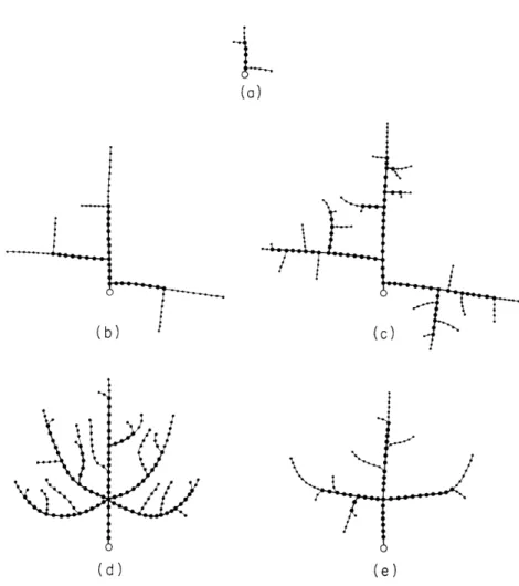
Fig. XX-8.

Several stages in the growth of a simulated branching

pat-tern (a-d). The persistence factors for growth and branching,

ST and STBR respectively, are both zero, so that both growth

and branching always follow the negative gradient of the local

density field.

An intermediate spacing of the branches is

caused by intermediate distances between branching points,

DBL for the distance from a basal branching point and DDL

for the distance from the distal end of the segment.

caused by low values of the limiting distances between branching points, DBL = 1.0 and DDL = 1.0. The tend-ency to assume a diffuse circular shape is obvious.

Fig. XX-10.

This treelike pattern is caused by increasing the limiting

distance from the distal end of the segments, DDL = 10. 0,

while maintaining the limiting distance from the basal end

at a low level, DBL

=

1.0.

Fig. XX-11.

A directed treelike pattern is generated

by biasing both growth and branching in

the direction of the Y axis.

(a)

\u)

>2

(d)

(e)

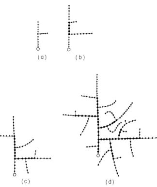
Fig. XX-12. (a-c) A hierarchically organized pattern is generated by having the limiting distances for branching vary with the total number of points in the pattern, NT. Both growth and branching are undirected.

NT range 0-20 20-100 100-200 DBL 1.0 8.0 1.0 DDL 1.0 1.0 1.0 Figure (a)

(d-e) These patterns are generated by the operation of a special branching rule once early in the generation process. This rule generates a number of branches symmetrically spaced in relation to the primary axis, and with equal angles between them. Growth is slightly biased upwards during some stage of the generation process to give a leaf-like pattern.

-i

I

(v) Branching may become directed in the same way as growth by introducing a bias in the local density field in any one direction in space or in the direction of a particular area or boundary. Growth bias and branching bias may be entirely independent, although they tend to reinforce each other if they are in the same direction. The whole pattern may thus be made to assume a directional asymmetric shape by growing and branching in a preferred direction.

Both growth and branching rules may have their parameters changed as a function of either some local property of the pattern or some property of the pattern as a whole.

This introduces a hierarchical element into the generation process, as required for the simulation of biological pattern generation. Thus, a specific branching subroutine may be applied only once at a particular early stage in the growth of the pattern which will determine the shape and relations of the primary branches of the pattern. Alternatively, the parameters may be a function of distance from a local perturbation in the growth space, which may result in specific morphogenetic effects of the perturbation. Also, branching may be completely inhibited in segments that have some particular connec-tivity characteristics, such as having a particular rank order, being a side branch to a main branch, or not having a free growing end, and so forth.

Results and Conclusions

Some representative examples of stages in the growth of the simulated patterns are shown in Figs. XX-8 through XX-12. Detailed descriptions and explanations are given in the legends for each figure or group of figures.

Note that in all figures a circle indicates the initiation point. Segments marked with a thick line are 'old' segments, i. e. , they no longer branch or grow.

Although preliminary in nature, our results seem to show the usefulness of the approach: First, by demonstrating the variety and richness of patterns that can be

gen-erated by a very limited set of adjustable parameters; second, by establishing an unam-biguous and quantitative method for investigating the generation process of an important

class of patterns; and third, by providing a working language for a synthetic approach to the problem of specification and classification of growing patterns in general.

D. Cohen

References

1. C. H. Waddington, New Perspectives in Genetics and Development (Columbia University Press, New York and London, 1962).