HAL Id: hal-00329412
https://hal.archives-ouvertes.fr/hal-00329412
Submitted on 22 Dec 2004
HAL is a multi-disciplinary open access
archive for the deposit and dissemination of
sci-entific research documents, whether they are
pub-lished or not. The documents may come from
teaching and research institutions in France or
abroad, or from public or private research centers.
L’archive ouverte pluridisciplinaire HAL, est
destinée au dépôt et à la diffusion de documents
scientifiques de niveau recherche, publiés ou non,
émanant des établissements d’enseignement et de
recherche français ou étrangers, des laboratoires
publics ou privés.
Distributed under a Creative Commons Attribution - NonCommercial| 4.0 International
License
of multi-satellite CLUSTER data
J. Soucek, Thierry Dudok de Wit, M. Dunlop, Pierrette Décréau
To cite this version:
J. Soucek, Thierry Dudok de Wit, M. Dunlop, Pierrette Décréau. Local wavelet correlation:
applica-tionto timing analysis of multi-satellite CLUSTER data. Annales Geophysicae, European Geosciences
Union, 2004, 22 (12), pp.4185-4196. �10.5194/angeo-22-4185-2004�. �hal-00329412�
SRef-ID: 1432-0576/ag/2004-22-4185 © European Geosciences Union 2004
Annales
Geophysicae
Local wavelet correlation: application to timing analysis of
multi-satellite CLUSTER data
J. Soucek1,2, T. Dudok de Wit2, M. Dunlop3, and P. D´ecr´eau2 1Institute of Atmospheric Physics, Prague, Czech Republic
2LPCE, CNRS and University of Orl´eans, 3A, avenue de la Recherche Scientifique, F–45071 Orl´eans cedex 2, France 3Space Science and Technology Department, CCLRC Rutherford Appleton Laboratory, Chilton, Oxfordshire OX11 0QX, UK
Received: 9 December 2003 – Revised: 31 August 2004 – Accepted: 9 September 2004 – Published: 22 December 2004
Abstract. Multi-spacecraft space observations, such as those
of CLUSTER, can be used to infer information about local plasma structures by exploiting the timing differences be-tween subsequent encounters of these structures by individ-ual satellites. We introduce a novel wavelet-based technique, the Local Wavelet Correlation (LWC), which allows one to match the corresponding signatures of large-scale structures in the data from multiple spacecraft and determine the rela-tive time shifts between the crossings. The LWC is especially suitable for analysis of strongly non-stationary time series, where it enables one to estimate the time lags in a more ro-bust and systematic way than ordinary cross-correlation tech-niques. The technique, together with its properties and some examples of its application to timing analysis of bow shock and magnetopause crossing observed by CLUSTER, are pre-sented. We also compare the performance and reliability of the technique with classical discontinuity analysis methods.
Key words. Radio science (signal processing) – Space
plasma physics (discontinuities; instruments and techniques)
1 Introduction
Consider a fleet of spacecraft that is crossing a plasma dis-continuity (e.g. a shock front, a large-scale structure), yield-ing a series of measurements that show resemblyield-ing patterns with different crossing times. The correct identification of these patterns and the resulting crossing times are key in-gredients for determining the orientation and the velocity of the discontinuity. This timing problem has received consid-erable attention in the analysis of multi-point measurements from the four CLUSTER (Escoubet et al., 1997) spacecraft.
Usual solutions to this timing problem involve direct visu-alization or, more exceptionally, correlation analysis between the different signals or explicit modeling (Paschmann and Daly, 1998; Haaland et al., 2004). The simplicity of these
Correspondence to: J. Soucek
approaches often stands out against the sophistication of the techniques used for later analysis, such as the inference of the spatial geometry of the plasma structures (Mottez and Chanteur, 1994). Timing problems are easy to handle when the same sharp discontinuity is observed by all satellites. This is sometimes the case with quasi-perpendicular shock crossings. Unfortunately, the situation quickly degrades as soon as the four spacecraft do not see the same structures, or if the discontinuity has a finite extension.
Our objective is to show that the concept of local correla-tion (Bendat and Piersol, 2000) can be successfully applied in such cases and is much more appropriate than classical correlation techniques that require a certain degree of sta-tionarity of the data. We introduce a local wavelet correla-tion (LWC) technique suitable for correlating non-stacorrela-tionary time series, such as those obtained from space plasma ex-periments. This multiscale method, based on the continuous wavelet transform (CWT), allows for a more flexible iden-tification of discontinuities, offering both higher resolution and better robustness. After a description of the method in Sect. 2, and of its properties in Sects. 3 and 4, we shall focus on a series of examples taken from CLUSTER data (Sect. 5) and make comparisons with other approaches.
2 The local wavelet correlation: description of the method
The timing problem described above is often solved using an ordinary time domain cross-correlation by choosing a sec-tion of each time series containing the structure of interest and shifting those two signals in time with respect to each other, until the cross-correlation of the shifted signals is max-imized. The time shift maximizing the correlation is then used as an estimate of the time lag between the observations of the same structure by the two satellites. This technique, however, requires that the time lag does not change within the correlation window. Since the time series under con-sideration are strongly non-stationary, this assumption is not
satisfied and the result depends significantly on the choice of this window. The local correlation technique described be-low is much better suited to analysis of non-stationary data and eliminates this major drawback of the traditional method. The concept of local correlation function (LCF) as a tool for correlating two time series f (t) and g(t) locally in the neighborhood of two fixed points (t1for f (t ) and t2for g(t ))
is well known from the classical literature on signal process-ing (Bendat and Piersol, 2000; Boashash, 1992). This local approach is perfectly appropriate for the timing analysis of strongly non-stationary data sets, like those shown in this article, where the correlation varies significantly over time. Due to the limited statistical content of the data, the question of the choice of the proper estimator of the local correlation is critical to the analysis.
In Perrin et al. (1999) the authors introduced a wavelet-based estimator of the local correlation and they applied it successfully to match stereoscopic images. A similar wavelet technique was described previously in Kawata and Arimoto (1996). In this article we introduce a similar wavelet based estimator of LCF, the local wavelet correlation (LWC), which is more appropriate for timing analysis of the time series from multiple spacecraft.
To estimate the LCF, we perform a multiscale decom-position using the Continuous Wavelet Transform (CWT), decomposing the time series into a set of components that contain information about the data at different scales. For each time step, we obtain a set of wavelet coefficients that uniquely describe the signal and its local properties at that time, such as the signal level, the slope, the smoothness, etc. If a similar pattern or structure appears at two different times, then the wavelet coefficients at these times of occur-rence should also match. The degree of matching thereby provides a measure of similarity between the two structures. At this point, no assumptions are made on what may cause dissimilarity (shock acceleration, spatial structures, ...). The procedure thus consists in taking a pair of records, comparing their wavelet coefficients pairwise and looking for possible coincidences. Structures that undergo modifications can still be recognized (Perrin et al., 1999), making the LWC really a pattern matching tool.
The LWC is a multiscale method in the sense that it op-erates simultaneously on different time scales (in contrast to the cross-correlation function, where the dominant scale is set by the length of the window). Indeed, the method auto-matically adapts itself to the dominant scales of the record: it focuses on small scales if the signal locally contains small-scale structures only, and on large small-scales otherwise. Sev-eral studies have shown that the human eye essentially pro-ceeds in the same way, always trying to extract the most rel-evant scales (Marr, 1982). Owing to this, the method can achieve a much better time resolution than classical correla-tion approaches, going as far as the sampling period. Further-more, by properly choosing the wavelet, one can automati-cally get rid of trends and offsets. All these properties make the method much more amenable to a systematic analysis of multi-satellite data.
Let f (t) and g(t) represent two time series to be compared and let their CWT be defined as (Daubechies, 1991; Mallat, 1998):
W[f ](a, τ ) = Z +∞
−∞
f (t )ψa,τ∗ (t ) dt , (1)
where ψa,τ(t ) is the base wavelet derived by shifting and
rescaling a chosen mother wavelet function ψ and * denotes complex conjugation. ψa,τ(t ) = 1 √ aψ ( t − τ a ) . (2)
The CWT can be understood as a generalization of the win-dowed Fourier transform in the sense that it yields the spec-tral decomposition of the signal as a function of time. The concept of spectral decomposition is more general in this context where various shapes of base functions may be used, but the wavelet scale a still roughly corresponds to the in-verse value of frequency 1/f , since it specifies the width of the base function. The most important advantage of the wavelet transform is its optimal trade-off between time res-olution and frequency resres-olution. Since the mother wavelet function ψa,τ(t )is localized in time and its effective width is
given by its scale a, each wavelet coefficient W[f ](a, τ ) car-ries information about the input signal f in a neighborhood of time τ , with the width of this neighborhood being pro-portional to the scale a. As the width of the neighborhood decreases with decreasing scale (increasing frequency), the time resolution increases, yielding the above mentioned rela-tion between spectral and temporal resolurela-tion.
In our study we shall use real wavelets, but the expressions remain valid for complex signals. Let us first normalize the wavelet coefficients at each time step τ , in order to remove any dependence of the LCF on the local signal power:
W[f ](a, τ ) = W[f ](a, τ ) / Z ∞
0
|W[f ](α, τ )|2dα
α . (3)
We then compute the cross-correlation between the normal-ized wavelet transforms of f (t ) and g(t ), as measured, re-spectively, at times t1 and t2. The definition of the LWC
simply reads γ (t1, t2) = Z ∞ 0 W[f ](a, t1) W ∗ [g](a, t2) da a . (4)
Values of the LWC range between −1 and 1 and can thus be interpreted as a measure of similarity between the func-tion f (t) in a neighborhood of the point t1and function g(t )
in a neighborhood of t2. Given a pattern that is observed in
f around time t1, we can say that it matches a similar
pat-tern observed in g around time t2if γ (t1, t2)exceeds a given
threshold. The difference δt =t2−t1then corresponds to the
time lag of interest.
The above definition is appropriate for the matching of any type of time series; for our purposes, it is often desirable to make the results more robust, at the expense of the time reso-lution, as we know that the time lag should not vary abruptly
in time. To do so, we slightly modify the definition of the LWC by averaging the integrand in Eq. (4) over a short time interval. This averaging first yields
s(t1, t2) = Z ∞ 0 da a Z 1τ −1τ W[f ](a, t1+τ ) W ∗ [g](a, t2+τ ) u(a, τ ) dτ , (5)
where the averaging is carried out over a two-dimensional window u(a, τ ); the constant 1τ defines the maximum width of this window. Finally, the LWC is obtained by nor-malizing the local correlation between −1 and 1
γ (t1, t2) = s(t1, t2) / s Z Z |W[f ](a, t1+τ )|2u(a, τ ) dadτ a · Z Z |W[g](a, t2+τ )|2u(a, τ ) dadτ a . (6)
The window u(a, τ ) should be designed consistently with the properties of the wavelet transform: its width in time should be proportional to the wavelet scale in order to keep the time-frequency resolution trade-off provided by the CWT. For example, such a window can be built from an arbitrary one-dimensional window function w(t ) (rectangular, trian-gular, Gaussian, etc.) by rescaling it proportionally to the wavelet scale a and normalizing the window so that the inte-gralR u(a, τ ) dτ remains independent of a:
u(a, t ) = 1
aw(t /a) . (7)
Using this window we achieve the goal of adapting the win-dow size to the wavelet scale but keeping equal weights for each scale.
The LWC can be tuned in several ways to the properties of a data set. The main parameters are: the choice of mother wavelet function ψ , the width and shape of the averaging window (given by 1τ and the function w(t ) in Eq. 7), and the upper and lower bounds aminand amax of the range of scales over which the wavelet coefficients are integrated.
In real world applications, one always deals with finite-length discretely sampled signals and a discrete form of the above expressions, in which integrals are replaced by sums. The resolution of the data already sets some limitations on the choice of the above parameters. A minimum value of
aminis determined by the sampling frequency to be approxi-mately equal to 2Tsamp, where Tsampis the sampling period. One may occasionally want to take a larger value of aminto discard small scales, which are easily affected by noise.
The maximum scale amaxshould be significantly smaller than the size of the data set, to reduce the impact of the boundary errors of the CWT. Such boundary effects, how-ever, can be significantly reduced by using wavelets that have a sufficiently large number of vanishing moments (N >4). With such wavelets, the CWT is invariant with
respect to polynomial trends of the order of N −1 (Mal-lat, 1998). We may therefore detrend the original data with a 4th order polynomial (forcing its value and its first derivative at the end points to vanish), to eliminate bound-ary effects without losing any pertinent information. Fi-nally, as is usual with the CWT, the scales a should be log-arithmically spaced. A good compromise between redun-dancy and computational burden is provided by the array
a=[amin, √
2amin,2amin, . . . , amax].
3 Application to timing analysis to satellite data
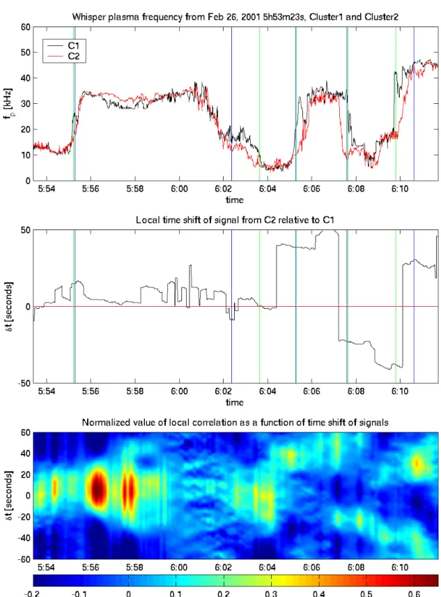
Before analyzing the timing of various CLUSTER data sets, let us first consider a test case that illustrates the properties and the potential pitfalls of the method. The data set consists of local electron plasma frequency measurements made by the WHISPER instrument (D´ecr´eau et al., 1997) on board the CLUSTER spacecraft during multiple magnetopause cross-ings – see the top panel of Fig. 1. Since the closely separated spacecraft are crossing the same discontinuities, both signals exhibit similar structures with a mere shift in time. Our final objective will be the accurate assessment of this time shift.
A visual inspection of the time series in Fig. 1 already sug-gests that the time lag continuously evolves in time (even changing sign). Note also that the two spacecraft rarely see the same type of structure, which makes the timing analysis quite a challenge here.
We estimate the time lag as follows: first the LWC is com-puted from the CWT using Eqs. (3), (5) and (6). The function
f (t )denotes the record from spacecraft C1 and g(t ) is from C2. Next, we compute the local correlation γ (t, t +δt ) for a range of lags −1T <δt<1T (where 1T is an upper bound set by the user) and for all the samples of the record. The re-sults are stored in a matrix which is displayed in the bottom panel of Fig. 1. For each time step, we now determine the lag δtmaxthat maximizes the local correlation. This will be our estimate of the timing difference; see the middle panel of Fig. 1. Note that the values of δtmaxare not restricted to inte-ger multiples of the sampling period, as better resolution may be achieved by locally fitting a parabola to the maximum of the LWC. In this example, the reference signal is from space-craft C1, so the results can be interpreted as the time it takes for patterns observed by C1 at time t to reappear at C2.
Before interpreting these results, let us comment on how the LWC analysis proceeds. As specified before, the LWC is data-adaptive in the sense that it automatically selects the range of scales in which the power content is the largest. At the magnetopause crossing of 06:05:20 UT, the dominant pattern is the step-like discontinuity, which affects all scales alike. The LWC clearly reaches a single and well-defined maximum with a peak correlation of 0.3. The value of corre-lation may seem rather low here, but note that the signals are significantly dissimilar in the neighborhood of the disconti-nuity (a decrease in density behind the crossing is seen only at C1). Regardless of this dissimilarity, the LWC identified the correct time lag between the fronts of the MP crossings.
Fig. 1. Example of LWC timing, applied to the electron density measured by WHISPER during repetitive magnetopause crossings on 26
February 2001, from 5:54–6:11 UT. The upper panel shows the plasma frequency as measured by spacecraft C1 and C2. The middle panel provides the time lag for which the LWC is maximum. Positive values imply that C1 is preceding C2. The bottom panel displays the LWC versus lag and time; the color scale ranges from −0.2 to 0.65. The approximate location of five magnetopause crossings are indicated by vertical green lines. In this example, 10th order Daubechies wavelets were used with a window derived from a 1-D Gaussian window.
A similar situation, where a correct time shift is identified correctly by a single sharp maximum of the LCF, occurs for the next crossing (06:08 UT).
A different situation occurs at 6:00 UT, where the LWC tries to lock on small scales associated with weak wave ac-tivity. The small amplitude of these fluctuations is not prob-lematic per se, since the wavelet coefficients are normalized versus local power. The main problem comes from the lack of similarity between the two records. Not surprisingly, the absolute value of local correlation remains rather low (typi-cally −0.1 to 0.1). It also exhibits multiple maxima and the estimated lag varies erratically. The concept of LCF is inap-plicable here.
4 Pitfalls and validation of the results
The preceding example reveals several potential pitfalls, whose understanding is the key to a proper interpretation of the LCF analysis results.
In the first place, we must stress that a time lag can be properly and unambiguously defined only for signals that are identical up to a shift in time. In the more realistic situation, when the signals are similar but not identical, pattern match-ing is required. A threshold must be selected below which the patterns are too dissimilar to justify the definition of a time lag. This occurs between 05:57 and 06:00 UT in Fig. 1. A different problem is raised by the magnetopause cross-ing at 05:55 UT. Spacecraft C1 observes in the middle of the ramp a small dip that goes unseen by C2. The LWC algo-rithm correctly matches the ramp of C2 with the first part of C1’s ramp, yielding a time lag of approximately 10 sec-onds. However, it fails to resolve the second part of the ramp, where the two signals almost coincide.
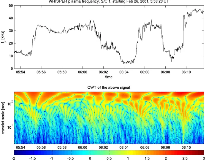
These effects are a direct consequence of the properties of the CWT. Each wavelet coefficient W(a, t ) contains in-formation about the input signal in a neighborhood of the point t . The width of this neighborhood is given by the wavelet width which is proportional to the scale. Discontinu-ities or abrupt changes in the signal contribute to wavelet co-efficients at a wide range of scales, analogously to a Fourier decomposition of a step function. The localization of this contribution in time is again given by the scale of the wavelet. In Fig. 2 the spiky structures corresponding to such disconti-nuities in the signal can be clearly recognized.
When the LCF is estimated using Eq. (5), we match 2-D arrays of wavelet coefficients. Obviously, the spiky struc-tures discussed above contribute very significantly to the re-sult, since they cover a wide range of scales. The presence of such structures may influence the wavelet coefficients at large scales (and consequently the LWC), considerably far from the discontinuity. Now assume that a relatively smooth structure appears in the signal at a time t, close to a sharp discontinuity at a time t0. The contribution of the nearby discontinuity at t0 to the wavelet transform at t may actu-ally be stronger than that of the smoother structure present at time t. Consequently, the LWC at the time t may reflect the
correlation of stronger nearby structures. These different ef-fects explain the behaviour of the LWC at the magnetopause crossing of 5:55 UT. They also explain the unusually high level of correlation that appears just after the magnetopause crossing, from 05:56 to about 05:58 UT. The signals here are barely correlated, but since their variance is low most wavelet coefficients are contaminated by the presence of the nearby magnetopause discontinuity.
Another consequence of this contamination is the appear-ance of multiple maxima of comparable magnitude in LCF. An example of this multi-modality appears in the magne-topause crossing at 06:10 UT (see Fig. 1). The correlation matrix (bottom panel) exhibits two ridges: one in the region of positive shifts, which corresponds to the true 06:10 UT crossing, and another ridge that is simply a consequence of the overlap from the previous magnetopause crossing. As one moves further away from the crossing, the overlap cor-relation becomes weaker and finally, the correct local maxi-mum gets selected. Again, the problem does not really come from the method itself, but from the comparison of two struc-tures that are dissimilar.
From the examples discussed above, it becomes evident that the peak value of the correlation is not a sufficient indica-tion of the reliability of the time shift estimate. Specifically, a high level of correlation may not correspond to a correct es-timate, since multiple possibilities of pattern matching often exist.
Most of the discussed effects can be significantly reduced by feeding physical information into the algorithm, such as the range of scales over which the LWC is integrated. Be-forehand, we need some independent criterion to assess the validity of the results. Two such criteria are proposed below.
4.1 First validation criterion: multi-wavelet statistics
The first validation criterion is based on the idea that the es-timated time shift should depend on the input signals only, and not on the wavelets1. Tests carried out on synthetic sig-nals indeed do not show significant differences between var-ious families of wavelets, with orders ranging from 4 to 20. Some noticeable exceptions are the Haar, the Morlet and the Gaussian hat wavelets, whose performance is systematically lower.
We built a statistical ensemble by computing the time shifts δt from a set of different wavelet functions and deter-mined the distribution function (histogram) of the multiple
δt for each time t. Such a histogram is shown in the bottom panel of Fig. 3. For strongly correlated structures, the time lags are independent of the mother wavelet and so the
his-1This is not exactly true: different families of wavelets
(Daubechies, symlets, Haar, Morlet, . . . ) will not capture the fea-tures of the data in the same way. The order of the wavelets also affects the outcome. Low order wavelets (say, N <4) are more suit-able for irregular signals, whereas large order wavelets offer a better resilience against trends.
Fig. 2. The continuous wavelet transform of the density data of spacecraft C1 from Fig. 1. The lower panel shows the logarithm of W(a, τ ).
The CWT was computed using 10th order Daubechies wavelets.
togram should exhibit a single narrow peak. The width of this peak can be quantified by its standard deviation:
smw(t ) = s
X wavelet s
(δt − δtmax)2p(t, δt ) , (8)
where p(t, δt ) is the empirical probability of observing a lag
δtat time t (estimated from a statistical ensemble described above) and δtmaxis defined as in Sect. 3.
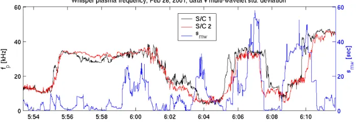
A necessary (but not sufficient) condition for the reliability of the time lag estimates is obtained by comparing the stan-dard deviation smw with a given threshold. Every time the value of smwexceeds this threshold the estimated time lags should be considered invalid. Figure 3 indeed shows that this criterion flags out the ambiguous magnetopause crossings at 06:05, 06:08 and 06:10 UT. With this criterion, however, the ambiguous magnetopause crossing between 06:02 and 06:04 is not rejected. That particular crossing does not suffer from multimodality, so an additional criterion is needed.
4.2 Second validation criterion: triangular differences
The second validation criterion is more specific to the CLUS-TER experiment with its four spacecraft arranged in a tetra-hedral configuration; it may also be adapted to other con-figurations. Given the four satellites, the time shifts can be estimated from 6 satellite pairs. Let 1tijdenote the time shift
from the signal of spacecraft i with respect to the signal of spacecraft j . Out of the 6 time shifts, only 3 are independent; their linear dependence can be expressed by the following set of equations:
1t21−1t31+1t32=0 (9)
1t31−1t41+1t43=0 (10)
1t42−1t41+1t21=0 (11)
1t32−1t42+1t43=0 . (12)
Geometrically, the above relations express the conservation of the oriented sum of the time shifts along the edges of each of the four sides of the tetrahedron, hence the name “triangu-lar differences”.
Fig. 3. The multi-wavelet criterion as applied to the density data of Fig. 1. The upper panel displays the density measurements, together with
the standard deviation smw. The bottom panel displays the histogram of the time shifts estimated using an ensemble of 15 different mother wavelets.
The application of the above relations to the validation problem is immediate: we compute all four left-hand sides of Eqs. (9–12) and compare them with a selected threshold. Note, however, that the time shifts are computed with re-spect to different reference signals. In Eq. (9), for example, the values 1t21 and 1t31 evaluated at time t give the time
shift relative to a structure appearing in signal 1 at the time
t. However, the same structure appears at time t+1t21in the
signal 2, and so the corrected form of Eq. (9) should actually read:
TD1=1t21(t ) − 1t31(t ) + 1t32(t + 1t21) =0 . (13)
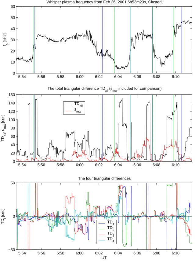
In Fig. 4 we plot the four triangular differences T Di
(bot-tom panel), as well as their sum T Dall=P4
i=1|T Di|
(mid-dle panel – black line). The smaller this quantity, the more consistent the lags are. One can check that all 6 time shifts are consistent for the magnetopause crossings at 05:55, 06:05 and 06:08 UT. The ambiguous crossing around 06:03 is now correctly identified.
When analyzing plasma discontinuities, it is desirable to know both the lag and the time of occurrence of the
discontinuity. For sharp discontinuities, this is straightfor-ward, as one simply takes the lag δt (tD)at the time when the discontinuity is strongest in the reference signal. If, how-ever, the discontinuity has a finite width, then the validation criteria can help by letting us take instead the time near the discontinuity when the lags are most reliable. These times are marked by the blue vertical lines in Fig. 4. Comparing them with the green lines obtained by visualization, we can check that the estimates are indeed consistent.
5 Estimating normal velocity vectors of discontinuities
We finally consider a series of examples where the LWC tim-ing is used to estimate the orientation and normal velocity of the Earth’s bow shock and the magnetopause. These results are compared to those obtained by standard methods (copla-narity and minimum variance techniques). All examples are based on the data collected by the four CLUSTER satellites when the latter were in an approximately tetrahedral config-uration, with a spacecraft separation of about 600 km.
5:54 5:56 5:58 6:00 6:02 6:04 6:06 6:08 6:10 0 10 20 30 40 50 60
Whisper plasma frequency from Feb 26, 2001 5h53m23s, Cluster1
f p [kHz] 5:54 5:56 5:58 6:00 6:02 6:04 6:06 6:08 6:10 0 20 40 60 80 100 120 140 160
The total triangular difference TD
all (smw included for comparison)
TD all , s mw [sec] TD all s mw 5:54 5:56 5:58 6:00 6:02 6:04 6:06 6:08 6:10 −50 0 50
The four triangular differences
TD i [sec] UT TD 1 TD 2 TD 3 TD 4
Fig. 4. The triangular differences between the time lags, as computed between all six satellite pairs. The data are the same as in Fig. 1. The
upper panel shows the density data from spacecraft C1 only. The bottom panel displays all four triangular differences. The sum TDall of the triangular differences, and the standard deviation smw are displayed in the central panel.
0 2 4 6 8 10 12 14 20 40 60 80 100 |B| [nT] time [sec]
Bow shock crossing on March 31, 2001, 19:00:38 − 19:00:50, FGM data
0 2 4 6 8 10 12 14 20 40 60 80 100 |B| [nT] time [sec]
The above dataset, time−aligned using LCF timing SC1 SC2 SC3 SC4 SC1 SC2 SC3 SC4
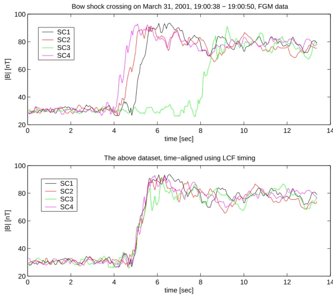
Fig. 5. A LWC analysis of a sharp, quasi-perpendicular bow shock crossing of 31 March 2001, from 19:00:38–19:00:50 UT. The upper panel
shows a magnetic field magnitude observed by the FGM instrument on CLUSTER during the bow shock crossing. The bottom panel shows the same data but with the shock fronts shifted by the lags obtained from the LWC. The sampling frequency of the magnetic field data is 22.5 Hz.
The normal velocity vector is inferred from the timing in-formation using the classical method (Paschmann and Daly, 1998; Dunlop et al., 2001): let 1tij denote the time shift
es-timated between signals from satellites i and j , as defined in Sect. 4.2. Let also ri denote the position of spacecraft i.
As-suming that the crossed boundary or structure is planar and moving with uniform velocity, we can now estimate its unit normal vector n and magnitude of normal velocity |V | by solving a simple set of linear equations:
1
|V |(ri −rj) ·n = 1tij(t ), i, j =1 . . . 4, i < j . (14)
In the case of four satellites this results in an overdetermined set of 6 linear equations with 3 unknowns, which can be solved using standard least-squares techniques.
The above method relies on the rather strong assumptions of planarity and uniform velocity. Recent studies based on
CLUSTER data (Horbury et al., 2002) suggest that in the case of terrestrial bow shock, and for a satellite separation of several hundred kilometers, the above assumptions are usually satisfied with reasonable accuracy. On the other hand, the magnetopause can still be approximated by a planar structure, but its acceleration is often significant enough to invalidate the uniform velocity approximation (Dunlop et al., 2001).
5.1 First example: quasi-perpendicular shock crossing
Figure 5 illustrates an application of the LWC timing to mag-netic field measurements obtained by the FGM magnetome-ter (Balogh et al., 1997) during a quasi-perpendicular bow shock crossing. The shock ramp is relatively steep and the profile is very similar on all spacecraft. Not surprisingly, the timing is well defined and no fine tuning is necessary. We
5:54 5:56 5:58 6:00 6:02 6:04 6:06 6:08 6:10 0 20 40 60 f p [kHz] / |B| [nT]
WHISPER plasma frequency and FGM magnetic field, 26/02/2001, Cluster 1
5:54 5:56 5:58 6:00 6:02 6:04 6:06 6:08 6:10 −1 −0.5 0 0.5 1 n x 5:54 5:56 5:58 6:00 6:02 6:04 6:06 6:08 6:10 −1 −0.5 0 0.5 1 n y 5:54 5:56 5:58 6:00 6:02 6:04 6:06 6:08 6:10 −1 −0.5 0 0.5 1 n z 5:54 5:56 5:58 6:00 6:02 6:04 6:06 6:08 6:10 0 20 40 60 80 time |v| [km/s] f p − WHISPER |B| − FGM n x − fp n x − |B| n x − fp n x − |B| n z − fp n z − |B| |v| − f p |v| − |B|
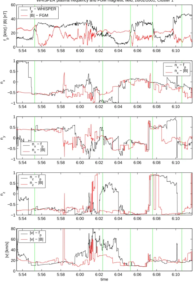
Fig. 6. Application of the LWC to multiple magnetopause crossings on 26 February 2001, from 05:53:30–06:11:30 UT. The upper panel
shows the input data from spacecraft C1: total magnetic field from FGM (resampled at 4 Hz), and plasma frequency from WHISPER (sampled at 2 Hz). Panels 2 to 4 display the three components of the normal vector n of the discontinuities as determined from the magnetic field and the electron density data. The bottom panel shows the magnitude of the velocity.
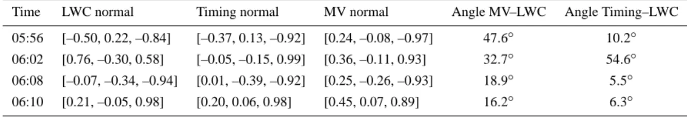
Table 1. Normals from various methods.
Time LWC normal Timing normal MV normal Angle MV–LWC Angle Timing–LWC
05:56 [–0.50, 0.22, –0.84] [–0.37, 0.13, –0.92] [0.24, –0.08, –0.97] 47.6◦ 10.2◦ 06:02 [0.76, –0.30, 0.58] [–0.05, –0.15, 0.99] [0.36, –0.11, 0.93] 32.7◦ 54.6◦ 06:08 [–0.07, –0.34, –0.94] [0.01, –0.39, –0.92] [0.25, –0.26, –0.93] 18.9◦ 5.5◦ 06:10 [0.21, –0.05, 0.98] [0.20, 0.06, 0.98] [0.45, 0.07, 0.89] 16.2◦ 6.3◦
used 10th order Daubechies wavelets. Averaging was per-formed over 52 logarithmically spaced wavelet scales from
amin=0.4 s to amax=30 s.
5.2 Second example: multiple magnetopause crossings
Let us now return to the multiple magnetopause crossings of 26 February 2001, which served before as a test case. Fig-ure 6 shows the normal components of the the magnetopause crossings (three panels in the middle) estimated using the LCF timing both from FGM magnetic field data and from WHISPER plasma frequency data. As before, green lines in-dicate the approximate locations of the magnetopause cross-ings.
Clearly, there is a good agreement between the normal es-timates based on the density data and on the magnetic field data for the crossings at 05:55, 06:08 and 06:10 UT. The discrepancies between the results for the other two cross-ings are a consequence of the problems described above in Sect. 4. Note that the two estimates often significantly differ and tend to agree only in the vicinity of magnetopause cross-ings, where significant correlated structures are present in all signals. This comparison of multi-instrument data represents an ultimate test of the correctness of the LWC technique.
Minimum variance analysis (Paschmann and Daly, 1998) is a single spacecraft technique for estimating the direction of a discontinuity normal from a magnetic field measure-ment. This method is completely independent from the inter-spacecraft timing technique, so we use it as another valida-tion test for the LCF timing-technique. The properties of this classical method are thoroughly studied in the literature (Paschmann and Daly, 1998). Like the timing based tech-niques, the minimum variance is known to suffer from errors introduced by deviation from the assumptions of planarity and time stationarity of the discontinuity, but the assumption of uniform velocity of the discontinuity is not used in this approach.
Table 1 summarizes magnetopause normals obtained by the two different techniques for the event of 26 February 2001 (see also Fig. 6). The second and third columns of the table contain normals computed from the timing information using Eq. (14). The second column normals use the timing obtained automatically by the LWC and in the third column the timing is estimated by traditional visual comparison and by manual shifting of data sets. The table also shows the
normal vector obtained by minimum variance and angles be-tween different normal estimates.
By comparing the LWC timing normals and the normals calculated from timing obtained by visual matching of data, we can evaluate the correctness of the LCF estimates. This comparison confirms the conclusions stated above: for all magnetopause crossings, except for the one at 06:02, the re-sults obtained from the LWC fully agree with the visual tim-ing observations. The relative angles between those normals range form 5◦to 10◦. In the case of the 6:02 crossing, the LWC technique fails, as was indicated by the validation cri-teria in Sect. 4 and the resulting normal is therefore incor-rect. Comparing the timing normals with minimum variance normals, we can deduce some information about the accel-eration of the magnetopause between the crossings by indi-vidual satellites. Following the approach by Dunlop et al. (2001), we assume that the magnetopause is approximately planar but its acceleration on the scale of spacecraft separa-tion may not be negligible. From Table 1, it is evident that for the last two MP crossings the minimum variance and timing normals agree within 20◦, so the assumptions of planarity and uniform velocity of the discontinuity are satisfied to a reasonable extent and Eq. (14) is applicable. On the other hand, the first crossing at 05:56 shows a significant deviation of 47.6◦ and we can conclude that this is either caused by an acceleration of the magnetopause or by a localized spatial structure.
6 Summary and conclusions
In this paper we introduced the Local Wavelet Correlation (LWC) as a novel tool for estimating the timing differences from multi-satellite data. This technique was designed to cor-relate input signals over a wide range of scales while putting equal weight on each scale. When applied to non-stationary signals, the LWC is more robust than ordinary linear correla-tion methods, which tend to be biased by large-scale struc-tures of the size of the averaging window. Secondly, the correlation coefficient can be calculated locally, yielding the level of correlation between two time series as a function time, with a very good time resolution.
The LWC was used here to determine the relative time shift between observations of the same plasma structures by
each of the four CLUSTER satellites. Tests based on a col-lection of events show that the LWC correctly matches sim-ilar patterns and provides consistent time differences when-ever these patterns can be unambiguously identified by eye. The method fails when the compared patterns become too dissimilar to justify a matching. We developed for that purpose two independent validation techniques, which allow one to determine the intervals in which the timing results are unreliable.
In the context of multi-point space plasma observations, timing information is essential for determining the orienta-tion and the normal velocity of the bow shock or the mag-netopause. Using several examples, we demonstrated that the results obtained by LWC are fully consistent with those obtained by classical methods. One major advantage of the LWC, however, is that it requires no guidance, making it more amenable to a systematic statistical study of large num-bers of discontinuity crossings.
Future work includes the possible application of this method to the timing of complex patterns containing sub-structures of different origin with possibly different veloc-ities. Here we can take advantage of the high time reso-lution of the LWC and the possibility to focus the corre-lation on a selected range of scales. A 2-D version of the LWC is presently under development for computing flow ve-locity fields from SoHO coronagraph images and for doing stereoscopic matching on image pairs from the future Stereo mission.
Acknowledgements. The first author was supported by Program for International Scientific Cooperation (PICS 1175), ESA PRODEX Contract No. 14529 and grant 205/01/1064 of Grant Agency of the Academy of Sciences of the Czech Republic.
Topical Editor T. Pulkkinen thanks two referees for their help in evaluating this paper.
References
Balogh, A., Dunlop, M. W., Cowley, S. W., Southwood, D. J., et al.: The Cluster magnetic field investigation, Space Sci. Rev., 79, 65– 92, 1997.
Bendat, J. S. and Piersol, A. G.: Random data, analysis and mea-surement procedures, Wiley, New York, 2000.
Boashash, B.: Time-frequency signal analysis – methods and appli-cations, John Wiley Press, New York, 1992.
Daubechies, I.: Ten lectures on wavelets, SIAM, 1991.
D´ecr´eau, P., Fergeau, P., Krasnoselskikh, V. et al.: WHISPER, a resonance sounder and wave analyser: Performances and per-spectives for the Cluster mission, Space Sci. Rev., 79, 157–193, 1997.
Dunlop, M. W., Balogh, A., Cargill, P., et al.: Cluster observes the Earth’s magnetopause: coordinated four-point magnetic field measurements, Ann. Geophys., 19, 1449–1460, 2001.
Escoubet, C. P., Russel, C. T., Schmidt, R. et al.: The Cluster and Phoenix Missions, Kluwer Academic Publishers, Dodrecht, 1997.
Haaland, S., Sonnerup, B. U. ¨O., Dunlop, M. W., Balogh, A., Hasegawa, H., Klecker, B., Paschmann, G., Lavraud, B., Dan-douras, I., and R`eme, H.: Four-spacecraft determination of magnetopause orientation, motion and thickness: Comparison with results from single-spacecraft methods, Ann. Geophys., 22, 1347–1365, 2004.
Horbury, T., Cargill, P. J., Lucek, E. A., Eastwood, J., et al.: Four spacecraft measurements of the quasiperpendicular terres-trial bow shock: Orientation and motion, J. Geoph. Res., 107, SSH 10–1, 2002.
Kawata, K. and Arimoto, S.: Signal matching using wavelet corre-lation, Electronics and Comm. in Japan, 79 (9), 23–34, 1996. Mallat, S.: A wavelet tour of signal processing, Academic Press,
London, 1998.
Marr, D.: Vision: a computational investigation into the human rep-resentation and processing of visual information, Freeman, New York, 1982.
Mottez, F. and Chanteur, G.: Surface crossing by a group of satel-lites: A theoretical study, J. Geoph. Res., 99, 13 499–13 508, 1994.
Paschmann, G. and Daly, P. W.: Analysis methods for multi-spacecraft data, Kluwer, Amsterdam, 1998.
Perrin, J., Torresani, B., and Fuchs, P.: A localized correlation func-tion for stereoscopic image matching, Traitement du Signal, 16, 3–14, 1999.