HAL Id: hal-00299061
https://hal.archives-ouvertes.fr/hal-00299061
Submitted on 1 Jan 2003
HAL is a multi-disciplinary open access
archive for the deposit and dissemination of
sci-entific research documents, whether they are
pub-lished or not. The documents may come from
teaching and research institutions in France or
abroad, or from public or private research centers.
L’archive ouverte pluridisciplinaire HAL, est
destinée au dépôt et à la diffusion de documents
scientifiques de niveau recherche, publiés ou non,
émanant des établissements d’enseignement et de
recherche français ou étrangers, des laboratoires
publics ou privés.
S. Hergarten
To cite this version:
S. Hergarten. Landslides, sandpiles, and self-organized criticality. Natural Hazards and Earth System
Science, Copernicus Publications on behalf of the European Geosciences Union, 2003, 3 (6),
pp.505-514. �hal-00299061�
Natural Hazards and Earth System Sciences (2003) 3: 505–514
© European Geosciences Union 2003
Natural Hazards
and Earth
System Sciences
Landslides, sandpiles, and self-organized criticality
S. Hergarten
Institute of Geology, University of Bonn, Germany
Received: 19 September 2002 – Accepted: 25 October 2002
Abstract. Power-law distributions of landslides and
rock-falls observed under various conditions suggest a relation-ship of mass movements to self-organized criticality (SOC). The exponents of the distributions show a considerable vari-ability, but neither a unique correlation to the geological or climatic situation nor to the triggering mechanism has been found. Comparing the observed size distributions with mod-els of SOC may help to understand the origin of the variation in the exponent and finally help to distinguish the govern-ing components in long-term landslide dynamics. However, the three most widespread SOC models either overestimate the number of large events drastically or cannot be consis-tently related to the physics of mass movements. Introduc-ing the process of time-dependent weakenIntroduc-ing on a long time scale brings the results closer to the observed statistics, so that time-dependent weakening may play a major part in the long-term dynamics of mass movements.
1 Power-law distributions in natural hazards
Some natural hazards have been recognized to exhibit scale-invariant size statistics. Earthquakes are the most prominent example. World-wide monitoring of seismic activity has led to extensive statistics concerning the frequency of earthquake occurrence. Gutenberg and Richter (1954) found that log10N (m) = a − b m, (1) where N (m) is the number of earthquakes per unit time in-terval with a magnitude greater than or equal to m, and a and
bare parameters. The Gutenberg-Richter law has been sup-ported by an enormous amount of data and has been found to be applicable over a wide range of earthquake magnitudes globally as well as locally. The parameter b slightly varies from region to region, but is generally between about 0.8
Correspondence to: S. Hergarten
(hergarten@geo.uni-bonn.de)
and 1.2 (Frohlich and Davis, 1993). In contrast, the param-eter a quantifies the regional seismic activity and thus varies strongly. The scale-invariant character of the Gutenberg-Richter law becomes evident if it is transformed into a sta-tistical distribution of the sizes A of the rupture areas that reads
N (A) ∼ A−b, (2)
where N (A) is the number of earthquakes per unit time inter-val with a rupture area greater than or equal to A. The theory behind this transformation was introduced by Kanamori and Anderson (1975); brief reviews are given in almost all text-books on seismology (e.g. Aki and Richards, 2002; Lay and Wallace, 1995) and in some books on fractals in earth sci-ences (e.g. Turcotte, 1997; Hergarten, 2002a).
Relations that quantify the number of events as a func-tion of their size, such as Eqs. (1) and (2), are frequency-magnitude relations. In this context, the term frequency-magnitude is not restricted to earthquakes, but an arbitrary measure of the size of an event. Equations (1) and (2) define cumulative frequency-magnitude relations since they refer to the num-ber of events above a given size and not to the numnum-ber of events within a certain interval of sizes.
The statistical distribution defined by Eq. (2) is a power-law distribution. In general, power-power-law distributions are not restricted to the sizes of areas; A may be replaced with any measure of the size of an object or an event. A power-law distribution is free of characteristic scales: If we compare the number of events of size A or greater with the number of events of size λA or greater where λ is an arbitrary factor, the numbers always differ by the same factor λ−b, regardless of the absolute size of the considered events. For this rea-son, power-law distributions are also called fractal or scale-invariant distributions. Discussing the inevitable limitations of scale invariance at small and large scales would go beyond the scope of this paper, but there is a variety of literature ad-dressing the properties of fractal distributions (e.g. Turcotte, 1997; Sornette, 2000; Hergarten, 2002a).
Forest fires are another example of power-law distributed natural hazards. In contrast to earthquakes, the fractal prop-erties of forest fires were recently discovered (Malamud et al., 1998). As a consequence, available statistics are rather poor compared to earthquake data. This concerns the num-ber of studied areas as well as the range of scales covered by the studies. There is still a considerable uncertainty about the validity of power-law distributions in forest-fire statistics and concerning the exponents b of the distributions. The range of exponents reported so far is 0.31 ≤ b ≤ 0.49, but due to the limited number of available data sets, this result must be con-sidered with some caution. However, the exponent b of forest fires is considerably lower than that of earthquakes. A lower exponent means that the decay of the distribution (Eq. 2) at large sizes is slower. In other words, the relative number of large events in forest fires is higher than it is in earthquake statistics.
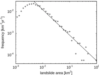
Concerning their statistical basis, landslides are between earthquakes and forest fires. Several studies addressing the frequency of landslide occurrence as a function of their size have been carried out, although the statistics still cannot com-pete with earthquake statistics. Apart from the fact that earth-quake monitoring has a longer history than making landslide statistics, the difference arises from different techniques of observation. While monitoring seismic activity is almost automatized, landslide statistics are mainly obtained from a combination of field work and analyzing aerial photographs. Extensive studies on fractal landslide statistics have been conducted since the 1990s. In a quite comprehensive study (Hovius et al., 1997), more than 7000 landslides in the west-ern Southwest-ern Alps of New Zealand were mapped. Figure 1 shows the resulting frequency-magnitude relation, obtained from those 4984 landslides located in the montane zone. It should be noted that the plot does not directly refer to a cumulative distribution according to Eq. (2), but repre-sents non-cumulative data in bins of sizes which increase lin-early with the event size (logarithmic binning). However, in case of a power-law distribution, both representations lead to straight lines with identical slopes in a double-logarithmic plot (e.g. Hergarten, 2002a). Therefore, the straight line with a slope of −1.16 suggests a power-law distribution with an exponent b = 1.16 in the cumulative sense.
A similar study performed in Taiwan (Hovius et al., 2000) resulted in a fractal distribution with b = 0.70. Later, the same authors (Stark and Hovius, 2001) investigated the ef-fect of censoring in the process of observation. As a result, they corrected the exponents to b = 1.46 (New Zealand) and
b = 1.11 (Taiwan), respectively. However, their approach is rather an improved fit of the data than a physically based model of censoring, and it may be biased as well as their orig-inal analysis (Hergarten, 2002a). In this sense, the modified exponents should not be overinterpreted; and the discrepancy shows that the uncertainty in determining the exponents is still large. Under this aspect, their results are in agreement with earlier studies.
More than 30 years ago, Fuyii (1969) found a power-law distribution with b = 0.96 in 650 events induced by heavy
10-4 10-3 10-2 10-3 10-2 10-1 100 frequency [km -2 yr -1 ] landslide area [km2]
Fig. 1. Frequency-magnitude relation obtained from landslide
map-ping in the central western Southern Alps of New Zealand (Hovius et al., 1997). The non-cumulative data were binned logarithmically. The straight line shows a power law with an exponent of 1.16.
rainfall in Japan. Even measuring the areas of landslide de-posits instead of those of the landslide scars leads to similar results; Sugai et al. (1994) obtained a power-law distribution with b = 1.0.
From some recent studies, exponents b which are larger than the values listed above have been obtained. Pelletier et al. (1997) compiled and analyzed landslide data from Japan (Ohmori and Sugai, 1995), California (Harp and Jib-son, 1995, 1996), and Bolivia. They obtained power-law dis-tributions over a quite narrow range (not much more than one order of magnitude in area) with exponents b between 1.6 and 2.0. Again, the quality of the power-laws is not suf-ficient for determining the exponent precisely; e.g. the ex-ponent from the California data was estimated to b = 1.6 first, but later to b = 1.3 (Guzzetti et al., 2002). Recently, rather comprehensive analyses of 16 809 landslides in Italy resulted in an exponent of about 1.5 (Guzzetti et al., 2002). A quite large exponent b = 2.3 was found for 709 earthquake-triggered landslides in Eden Canyon, California (Malamud and Turcotte, 1999).
In summary, there is evidence for fractal statistics in land-slides. Figure 2 compares the observed range of exponents with those of earthquakes and forest fires. The variation in the exponents of landslide size distributions is stronger than in the two other examples. We have already seen that a part of the variation may arise from statistical fluctuations or from applying different methods. The findings discussed above suggest that these uncertainties may amount up to a differ-ence δb ≈ 0.4.
Taking into account this uncertainty, it may be reasonable to assume a range of b between about 1 and 1.6 since the majority of the results falls into this range. The exponents of landslide distributions seem to be larger than those of earth-quakes in the mean. Therefore, the relative importance of large landslides is lower than it is in the example of
earth-S. Hergarten: Landslides, sandpiles, and self-organized criticality 507
0 0.5 1 1.5 2
exponent b
forest fires earthquakes
rockfalls
landslides
BTW model OFC model
forest-fire model
Fig. 2. Power-law exponents of the cumulative size distribu-tions of some natural hazards (upper part) and results of the most widespread self-organized critical models (lower part). The tick-marks refer to the studies on landslides mentioned in the text, the rockfall data analyzed and reviewed by Dussauge-Peisser et al. (2002), the four forest-fire data sets analyzed by Malamud et al. (1998), and 38 earthquake catalogs from various geographic regions (Frohlich and Davis, 1993, Table 1, last column).
quakes and much lower than in the example of forest fires. Geology, climate, type of landslides, and triggering mech-anisms seem to be good candidates to account for the ob-served variations in the power-law exponents. However, none of them has been clearly recognized to affect the land-slide size distribution. The number of available studies seems to be too low for a systematic analysis of the variety of po-tential influences.
A few studies address the triggering mechanism. Among the data discussed above, there are two data sets of earthquake-triggered landslides. One of them is that with the highest exponent b = 2.3 (Malamud and Turcotte, 1999), while the other leads to lower exponents of 1.6 or 1.3, respec-tively (Pelletier et al., 1997; Guzzetti et al., 2002). Although these values may suggest that the power-law exponents of earthquake-induced landslides tend to be higher than for hy-drologically triggered events, the statistics are not sufficient to provide a sound basis of such a speculation. In the study of the Italian landslides (Guzzetti et al., 2002), a second data set of 4233 landslides triggered by just one rapid snow melt event was considered, too. No significant difference concern-ing their size distribution compared to the long-term inven-tory was detected. Although the triggering mechanism may be crucial for the total number of landslides per time, its in-fluence on the size distribution seems to be negligible.
Due to the limited statistics, deriving reliable size distribu-tions for different types of landslides is difficult. Frequency-magnitude relations of rockfalls, a type of gravity-driven mass movements which strongly differs from most other types (e.g. slides in the strict sense or flows) have been in-vestigated in several studies. Dussauge-Peisser et al. (2002) compiled data on the sizes of rockfalls from various sources, obtaining power-law distributions for the rockfall volume
10-3 10-2 10-1 100 100 101 102 103 104 105 cumulative probaility P n number of fissions n q = 0.400 q = 0.490 q = 0.499 q = 0.500 q = 0.501 q = 0.510 q = 0.600
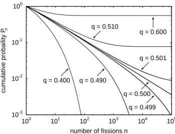
Fig. 3. Cumulative size distribution of a nuclear chain reaction
re-leasing two neutrons per fission for different values of the fission-ating probability q. A power-law distribution occurs at the critical point q =12.
with exponents between 0.4 and 1.0. Although these val-ues show a strong variability, a relationship to the geolog-ical setting was not found. Assuming that rockfall volume is proportional to A32, i.e. that small and large rockfalls are
geometrically similar, the volume distribution can be trans-formed to areas (Eq. 2) with exponents b in a range between about 0.6 and 1.5. As illustrated in Fig. 2, this range is not much smaller than that of landslides, but the exponents of rockfalls seem to be smaller than those of landslides in the mean. As a consequence, the relative importance of large events in rockfall statistics is more pronounced than in land-slide statistics, although still less than in the size distributions of forest fires.
Understanding the origin of the power-laws in mass move-ment statistics is a major challenge, both from a theoretical point of view as well as for hazard assessment. This aim leads from statistical descriptions towards physically based models. As a second step, it should be examined whether the observed variability in the power-law exponents is real or whether there is a universal value for all kinds of gravity-driven mass movements. In the first case, models may be helpful to attribute the variations to any kind of geological or climatic conditions.
2 Self-organized criticality
Power-law distributions are often attributed to critical phe-nomena. In classical thermodynamics, the existence of criti-cal points has been known for a long time. Instead of going into the theory of critical phenomena, let us consider a quite simple example of a nuclear chain reaction, which we will take as a prototype of an avalanche. Assume that a nucleus is fissionated, and that this process releases two neutrons. Each of these neutrons may fissionate another nucleus at a given
probability q. This process releases further neutrons (up to four), and so on, so that avalanches may occur. The statisti-cal distribution of these avalanches strongly depends on the parameter q which is related to the density of fissionable ma-terial in the considered sample. This model can easily be simulated on a computer or even be solved analytically in major parts. The resulting size distribution of the avalanches is given in Fig. 3 for some values of q; Pndenotes the prob-ability that an avalanche involves at least n nuclei.
The behavior changes drastically at q = 12. For q < 12, the probability of large avalanches decreases rapidly, so that the avalanches are in fact limited in size. This situation is called subcritical. On the other hand, Pn does not tend to-wards zero in the limit n → ∞ if q > 12. In this case, a certain fraction of fissions causes chain reactions of infinite size, although this is, strictly speaking, only true for infinite samples. This unstable situation is denoted overcritical. The situation where q = 12 is called critical point; it is charac-terized by a power-law decay of the event size distribution which indicates fractal properties. In the critical state, events of all sizes occur, and their statistical relationship is scale-invariant.
In this sense, considering the examples of natural hazards discussed in Sect. 1 in the context of critical phenomena is tempting. However, there is one major problem: Bring-ing the system to its critical point requires a precise tunBring-ing. In the model considered above, the size distribution of the avalanches considerably deviates from a power law even if q slightly deviates from its critical value. So why should the land surface be tuned to a hypothetic critical point almost everywhere on earth?
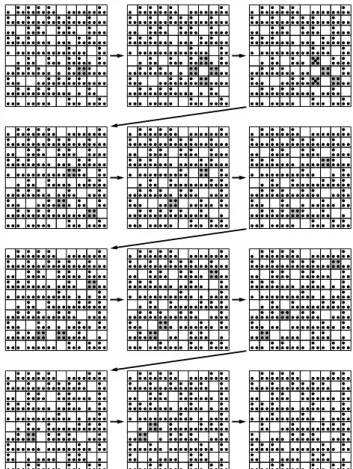
This is the point where the idea of self-organized critical-ity (SOC) starts. Fifteen years ago, Bak et al. (1987, 1988) found a system which organizes itself towards a critical state without any tuning. This system is a simple cellular automa-ton defined on a two-dimensional, quadratic lattice. Each site may be occupied by a number of grains (or any other objects, the physical context of these objects is not important for the model). In each step of the model, a grain is added to a ran-domly chosen site. If this site still contains no more than three grains, nothing happens, and another site is selected for a grain to be added. If, in contrast, the site contains four grains, it becomes unstable, and these four grains are redis-tributed among the four adjacent sites. Grains passing the boundaries of the model domain are lost. Afterwards, some sites may contain four or even more grains; they are relaxed by redistributing four grains according to the same rule. This may lead to avalanches; Fig. 4 shows an example. During the avalanche, 28 sites became unstable; and it took 11 re-laxation cycles until all sites became stable again. A total of 27 sites participated in the avalanche; so one cell became unstable twice.
This model is called Bak-Tang-Wiesenfeld (BTW) model. Its properties are discussed in every book on SOC (e.g. Bak, 1996; Jensen, 1998; Hergarten, 2002a). It was found that the BTW model organizes towards a state where the mean density (number of grains per site) fluctuates around a value
Fig. 4. Example of an avalanche in the Bak-Tang-Wiesenfeld model. Grains are represented by dots; unstable sites are marked with grey. The avalanche starts from one cell containing four grains and ceases after 11 relaxation cycles.
of about 2.1. This result is independent of the initial con-dition, so that the model in fact self-organizes towards this state. This state was found to be critical, i.e. the sizes of the avalanches are power-law distributed. This led to the term self-organized criticality which seems to have become some kind of magic word in several fields.
If transferred to a cumulative size distribution (Eq. 2), the exponent of the obtained distribution is very low. Measur-ing avalanche sizes in terms of the number of affected sites leads to b = 0.05. This value is much lower than the expo-nents of the power-law distributed natural hazards discussed in Sect. 1. In other words, the BTW model generates too many large events compared to earthquakes, landslides, rock-falls, and forest fires.
The forest-fire model is even simpler than the BTW model. Strictly speaking, several different forest-fire models were developed in the 1990s. SOC was discovered in the model introduced by Drossel and Schwabl (1992). Today, a slightly modified version (Grassberger, 1993; Clar et al., 1994) is mostly referred to; it is based on the following rules: Each site (of a mostly two-dimensional, quadratic lattice) is either empty or occupied by a tree. In each step, θ sites are ran-domly selected. Those of them which are empty give rise to
S. Hergarten: Landslides, sandpiles, and self-organized criticality 509
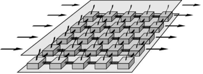
Fig. 5. Setup of a two-dimensional spring-block model. Blocks
are connected with each other and with a rigid driver plate through springs and leaf springs, respectively.
new trees. Then, a randomly chosen site is ignited. If this site is occupied by a tree, this tree and the cluster of trees connected to it is burned down.
The forest-fire model exhibits SOC in the limit θ → ∞, which means that the rate of ignition is low compared to the rate of tree growth. However, there is still uncertainty about the size distribution of the burnt clusters of trees. For fi-nite values of θ , the distribution significantly deviates from a power law at large event sizes, which makes the extrapolation for θ → ∞ difficult. Thus, there is still a strong variation in the estimated exponents b. Interestingly, the range is marked by recently published results, from b = 0.08 (Pastor-Satorras and Vespignani, 2000) to b = 0.45 (Schenk et al., 2002). Very recent results (Hergarten, 2002b) suggest b = 0.20, but raise doubts whether the forest-fire model fits into the frame-work of SOC because the destruction of trees is governed by a second class of fires which is exponentially distributed. In summary, the exponents b of the forest-fire model seem to be smaller than those obtained from nature. However, the dis-crepancy is not so strong that one should conclude that the forest-fire model is not at all applicable to forest fires.
The Olami-Feder-Christensen (OFC) model is the third widespread SOC model. From its physical background it be-longs to a large class of spring-block models developed for understanding the dynamics of earthquakes. Figure 5 shows the setup of a two-dimensional spring-block model.
The first spring-block model was introduced by Burridge and Knopoff (1967); numerous other followed which are more or less similar in their spirit. A review is given, e.g. by Turcotte (1999). Blocks are connected with each other and with a rigid driver plate through springs and leaf springs, respectively. They are held at their position by the static fric-tion at the bottom. The forces acting on the blocks are uni-formly increased by slowly moving the upper plate. As soon as the force acting on any block exceeds the maximum static friction, this block becomes unstable and is displaced. As a result, the forces acting on its neighbors change, which may give rise to avalanches.
The OFC model is a cellular automaton realization of such a model. Due to its fundamental character in the framework of SOC, it is discussed in all books on this field, too. Us-ing non-dimensional variables, its rules can be written in the form:
(i) Long-term driving as long as all blocks remain stable:
∂ui
∂t =1 as long as ui <1. (3)
(ii) Instantaneous relaxation of unstable blocks:
uj →uj+α ui for j ∈ N (i)
ui →0
if ui ≥1. (4)
For simplicity, the blocks are numbered with a single index
i, and N (i) denotes the nearest neighborhood of the block
i. The variable ui is the force acting on block i, normalized with respect to the maximum static friction force. The trans-mission parameter α depends on the strengths of the springs; it is not larger than14.
When the model was introduced (Olami et al., 1992), it was not essentially new, but OFC recognized the role of the upper leaf springs which connect the blocks to the upper plate not only for long-term driving, but also for the relaxation of unstable blocks. If a block is relaxed, a part of the force ui is transferred to the neighbors. Apart from boundary sites, this part is 4α. If the upper leaf springs are weak compared to the springs between the blocks. α converges to 14, so that the total amount of force is preserved during the relaxation. This case is denoted conservative limiting case; it was inves-tigated by Brown et al. (1991) and Matsuzaki and Takayasu (1991) before OFC published their results. However, it leads to a power-law size distribution with an exponent b = 0.23 (e.g. Hergarten, 2002a), which is too low compared to real earthquakes.
In case the upper springs are of finite strength, a certain amount of force is transferred to the driver plate, so that the relaxation rule is non-conservative. OFC recognized that the model still exhibits SOC in the non-conservative regime, but that the power-law exponent strongly depends on the level of conservation, i.e. on the parameter α. If all springs are identical α takes the value15. In this case, the exponent seems to be close to 0.7 (e.g. Hergarten, 2002a). For smaller values of α, the results apparently approach the range of b (between 0.8 and 1.2) observed in nature, although recently evidence for a universal value b ≈ 0.8 which is independent of α (at least for α ≥ 0.17) was found (Lise and Paczuski, 2001). No matter where this discussion will lead to, the OFC model has become a powerful tool for understanding the scale-invariant statistics of earthquakes.
3 Are landslides sandpile avalanches or earthquakes?
Two out of the three natural hazards discussed in Sect. 1 can be related to SOC with the help of the fundamental models discussed in the previous section: The OFC model (and sim-ilar spring-block models, too) has become a valuable tool in seismology, and the results of the forest-fire model are not too far of from the fire size statistics observed in nature, al-though the model may be somewhat oversimplified.
Thus, the idea of understanding fractal size distributions of landslides and rockfalls within the framework of SOC is
tempting. The models discussed in the previous section de-scribe of avalanching processes. The idea of avalanching was introduced into the theory of slope stability long ago. Bjer-rum (1967) found that instability in clays often does not oc-cur at the entire slip surface simultaneously, but starts from a small region. Slip occurring there destabilizes the neighbor-hood, so that instability may propagate. This phenomenon is called progressive slope failure; it seems to be quite similar to the spreading of avalanches in the fundamental models of SOC.
Interestingly, the BTW model is often called the sandpile model. However, if we recall its rules, we immediately rec-ognize that its relationship to sandpile dynamics is rather vague. The stability of a sandpile mainly depends on the local slope gradient, but not on the absolute number of sand grains at any location as assumed in the BTW model. Thus, the stability criterion of the BTW model hinges on the abso-lute surface height rather than on the slope gradient.
With respect to its applicability to landsliding, a second problem arises from the long-term driving mechanism. In nature, tectonic uplift and fluvial incision are the main coun-terparts to erosive processes. While the latter in general re-duce surface heights and slope gradients, the former are able to increase heights and gradients, so that finally a long-term equilibrium may be achieved. In this sense, tectonic up-lift and fluvial incision are the long-term driving processes of erosion and gravity-driven mass movements. In contrast, the BTW model is driven by randomly adding grains, which cannot be directly related to either tectonic or fluvial pro-cesses. In fact there is a second interpretation of the BTW model where the model variable does not describe a num-ber of grains, but a slope gradient (Bak et al., 1988; Jensen, 1998). This interpretation fixes these problems partly. But even if a physically consistent relationship between the BTW model and landform evolution could be found, the quantita-tive results are disheartening: The value b = 0.05 obtained from the BTW model is far away from the range observed for landslides and rockfalls in nature.
However, we may try to keep at least the essence of the sandpile idea. Let us start from a quadratic lattice where the state of each site is characterized by a surface height. Let
1i be the absolute value of the slope gradient at the site i. In order to keep the model as simple as possible, it is as-sumed that a site becomes unstable if its slope gradient 1i reaches a given critical value 1c. In this case, material shall move in downslope direction towards the nearest neighbors until 1i has decreased to a given residual slope gradient 1r. Some further simplifications are necessary in order to derive a simple relaxation rule from these assumptions (Hergarten, 2002a), finally leading to
1j →1j+14(1i−1r) for j ∈ N (i)
1i →1r
if 1i ≥1c. (5)
Both the parameters 1rand 1c can be eliminated from the relaxation rule and from the stability criterion by introducing
the variables
ui =
1i−1r
1c−1r
. (6)
This leads exactly to the stability criterion and the relaxation rule of the OFC model (Eq. 4), except for the parameter α occurring there. Instead of a parameter describing physical properties of the system, the relaxation rule of this simpli-fied landslide model has a constant transmission parameter of 14. This corresponds to the conservative limiting case of the OFC model.
As all SOC models, this landslide model needs some kind of long-term driving. Otherwise, the slopes will decrease through time and landsliding will cease. Interpreting the size distribution of landslides in the context of SOC requires that the slopes are maintained over long times, so that a long-term equilibrium between the dissipative process of landsliding and driving can be achieved. In the simplest approach, long-term driving is introduced by homogeneously tilting the sur-face, as it may result from tectonic uplift at large scales. As a result, the slope gradients increase uniformly through time. By rescaling the time axis of the model, the driving rule of the OFC model (Eq. 3) can be exactly reproduced.
In summary, this simple landslide model coincides with the conservative limiting case of the OFC model. The model seems to be physically reasonable, although somewhat over-simplified. The strong analogy to the OFC model may be surprising; it is at least a good example for different model approaches finally leading to the same mathematical model.
However, the quantitative results are again disappointing. As mentioned in the previous section, the model exhibits SOC, but the exponent b = 0.23 is significantly too low com-pared to landslides and rockfalls in reality. Comcom-pared to the BTW (sandpile) model, the results are better, but the over-estimation of the number of large events is still too large for any serious application to gravity-driven mass movements.
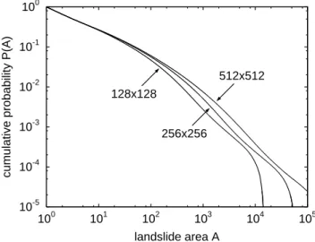
Blaming the poor results on the oversimplification of the physical model is tempting. However, this is somewhat dan-gerous: Points where the model is oversimplified are read-ily found, but finding out whether spending more effort on these aspects improves the results is often difficult. For in-stance, long-term driving by uniformly tilting the surface ap-pears to be unrealistic since it may describe large-scale tec-tonic processes, but disregards fluvial erosion. As a result, the surface will evolve towards one large slope, while flu-vial erosion generally subdivides it into a pattern of smaller slopes. This problem can be either fixed by coupling a model of fluvial erosion or by restricting the model scale to indi-vidual slopes and use simple assumptions for fluvial incision there. For simplicity, we switch towards individual slopes and assume a constant rate of fluvial incision at some edges of the model domain. The model can easily be modified in this way; it turns out that the driving rule (Eq. 3) must not be applied to all sites then, but only to those at the bound-aries where the river acts (Hergarten, 2002a). Figure 6 gives the size distribution obtained from simulating this model on
S. Hergarten: Landslides, sandpiles, and self-organized criticality 511 10-5 10-4 10-3 10-2 10-1 100 100 101 102 103 104 105
cumulative probability P(A)
landslide area A 128x128
256x256
512x512
Fig. 6. Landslide size distribution obtained from the sandpile-like
model under long-term driving by fluvial incision. The landslide sizes are measured in terms of the number of affected sites. The different curves correspond to lattices of different sizes.
quadratic lattices assuming that fluvial incision takes place at two adjacent edges.
At landslides sizes above about 100 sites, the distributions show a rough power-law behavior within a narrow range of scales (less than two orders of magnitude in area) with an exponent of about 1.2. This value fits well into the range il-lustrated in Fig. 2. However, the quality of the power laws is poor, and the shape of the distribution depends on the size of the lattice. As the size of the lattice is related to the size of the considered slope and the spatial resolution, this result is not very promising. In fact, a more detailed analysis (Her-garten, 2002a) has shown that the power-law behavior is a spurious effect of considering cumulative distributions and vanishes if the data are plotted in a non-cumulative diagram. Thus, assuming long-term driving by fluvial incision makes the results even worse, at least if it is introduced in this sim-ple form.
The problems might arise from disregarding the triggering mechanisms of landslides, such as rainfall, snow melt, and earthquakes. However, as discussed in Sect. 1, available data do not indicate any correlation between the size distribution and the triggering mechanism. Since SOC models often yield surprising results, incorporating triggering mechanisms into the model might improve the results, but this seems not to be very likely.
Effects of inertia are another candidate. In real sandpile dynamics, effects of inertia are quite important. As soon as a sandpile exceeds a critical size, grains toppling down-slope pick up enough kinetic energy to set many other grains in motion. As a result, the SOC behavior is lost then; the power-law distribution turns into a distribution where large events are preferred. As it makes the overestimation of large avalanches even worse, this is still not what we are looking for.
So there seems to be a fundamental problem with the
sand-Fig. 7. Setup of a spring-block model placed on a tilted plate.
pile-like landslide model which hinges on the conservative character of the conservation rule. The power-law expo-nents of earthquakes and landslides are not far away from each other, and the non-conservative OFC model has been successfully applied to earthquakes. Thus, relating the non-conservative OFC model to landslides might be the major step towards understanding landslide dynamics in the con-text of SOC. However, the conservative character of the re-laxation rule is closely related to the conservation of mass during an event (Hergarten, 2002a), so it seems to be im-possible to derive a non-conservative relaxation rule from a sandpile analogy.
So let us for the moment switch to an entirely different view on the landsliding process. If we assume a distinct slip surface, as it is present in translational and rotational slides, we may consider the forces acting on this surface. A spring-block model placed on an inclined plate (Fig. 7) may be the simplest physically reasonable description of this situation. However, the sketch immediately reveals the major problem of this approach, apart from the question how long-term driv-ing is realized: The drivdriv-ing force actdriv-ing on the blocks results from the inclination of the lower plate, but not from an addi-tional driver plate as in the original setup illustrated in Fig. 5. As a consequence, the upper leaf springs have vanished, and this makes the relaxation rule conservative. Thus, this model suffers from the same problem as the sandpile analogy, al-though the physical background of both approaches is en-tirely different.
In summary, neither the sandpile analogy nor the transfer of spring-block earthquake models to landslide or rockfall dynamics works on a quantitative level.
4 The role of time-dependent weakening
The findings of the previous section suggest that the sur-face gradient alone cannot be responsible for the fractal size statistics of landslides in a sandpile-like model; there must be another component. In principle, this result is not sur-prising since it is well-known that landslide abundance does not increase constantly with the terrain gradient in any given
area. Often, steep slopes which are more stable than ad-jacent slopes with a lower gradient are found. In general, slope stability depends on a variety of influences beside the gradient. Skipping everything except for the slope gradient was a first approach which has turned out to be too simple; we must introduce a second component in the model. The most straightforward idea is assigning the second component to the mechanical properties of the soil or rock which may change through time.
Early approaches in this direction were developed for dif-ferent topics in landform evolution. Bouchaud et al. (1995) introduced a two-state approximation for modeling sandpile dynamics. Grains are assumed to be either at rest or rolling with a pre-defined velocity; so the evolution of the sandpile is governed by both the slope gradient and the number of rolling grains. On a larger scale, a similar approach was introduced for modeling erosion processes (Hergarten and Neugebauer, 1996). Here, grains are assumed to be either tightly connected to their neighbors or mobile; the number of mobile grains is the second variable beside the slope gradi-ent. Later, this approach was transferred to landslide dynam-ics by replacing the number of loose grains with an amount of mobile material (Hergarten and Neugebauer, 1998, 1999). Although this approach is based on partial differential equa-tions, which makes it numerically demanding, it results in a fractal size distribution over a reasonable range of scales with exponents b close to unity. However, criticality occurs only within a quite narrow range of parameter combinations, so that the model behavior is somewhere between SOC and (tuned) criticality in the classical sense.
At the same time, Densmore et al. (1998) introduced an approach to landsliding as a component of a rather compre-hensive landform evolution model. Similar to the approaches discussed above, slope stability is governed by two compo-nents. One of them describes the surface geometry, while the other uniformly increases through time and introduces some kind of weakening. Instability occurs as soon as the sum of both components exceeds a given threshold. However, the landslides do not propagate in this model like the avalanches in the sandpile model; instead an explicit rule for their size was introduced. Motivated by experiments (Densmore et al., 1997), it is assumed that the size of a landslide being initi-ated at a certain location depends on the time span since the previous landslide at the location. The model yields power-law distributions with realistic exponents for the landslide volumes, but clean power laws can be recognized only over about one order of magnitude in landslide volume, which is in fact a very narrow range.
The idea of time-dependent weakening can be applied to both the sandpile-like model and the spring-block model by introducing a time-dependent criterion of stability instead of the condition ui < 1. The simplest time dependence con-cerns a linearly decreasing threshold, so that the slope re-mains stable as long as ui < 1 − λτi where τi is the time span since the last event at the site i and λ is a parame-ter characparame-terizing the rate of weakening. This approach is quite similar to that introduced by Densmore et al. (1998).
This criterion cannot be realistic on a long time scale as the threshold decreases to or even below zero through time. This means that every site will finally become unstable, even if its slope gradient is zero. But still more severe, this model was shown to exhibit SOC only in the trivial limiting case where time-dependent weakening becomes negligible (Hergarten and Neugebauer, 2000), at least under driving by tilting the slope. The case of long-term driving by fluvial incision was recently investigated (Hergarten, 2002a). A clean power-law distribution was not observed; the results are rather complex and considerably affected by the grid size. Thus, assuming a linearly decreasing threshold does not provide any new in-sights compared to the simple sandpile-like model or the sim-ple spring-block model.
The approach involving time-dependent weakening is some kind of two-variable model, while the established SOC models involve just one variable. The second variable is the time span τi since the last event at the site i. Obviously, τi increases through time according to ∂τi
∂t =1, which exactly coincides with the driving rule of the OFC model (Eq. 3). As soon as the site i becomes unstable, τi is reset to zero. This rule can also be related to the the relaxation rule of the OFC model (Eq. 4);i it is the completely dissipative limiting case
α =0 where transfer to the neighbors is inhibited. Thus, the two-variable model involving time-dependent weakening is a combination of two OFC models where one is conserva-tive, while the other is entirely dissipative. Both models are coupled by the criterion of stability which consists of a linear combination of the variables:
ui+λ τi <1. (7) There are several other ways of combining two variables than this one. Using the product of both variables according to
uiτi < µ (8)
is simple, too. According to this criterion, the threshold of in-stability decreases through time likeτ1
i. Transferred to slopes
(Eq. 6), the product criterion means that the slope remains stable as long as
1i < 1r+
µ (1c−1r)
τi
. (9)
Even a very steep slope would be stable immediately after a landslide. However, this is a merely theoretical problem as the gradients decrease during a landslide, so that they cannot be very high immediately after an event. After a sufficiently long time, each slope which is steeper than the residual slope
1rbecomes unstable, while shallower slopes will remain sta-ble forever.
The product approach was recently investigated, too (Her-garten and Neugebauer, 2000; Her(Her-garten, 2002a). It was found to differ strongly from the linear combination (Eq. 7). The model shows SOC, and the exponent b of the size dis-tribution is close to unity. This result is independent of the parameter µ and holds for driving by tilting the slope as well as for driving by fluvial incision. Thus, the model predicts
S. Hergarten: Landslides, sandpiles, and self-organized criticality 513 SOC with a universal power-law exponent which is within
the range observed in nature, but it cannot explain the ob-served variability. Combining both variables to a more com-plex criterion of stability such as
ui(1 + λ τi) < µ (10)
might be the next step.
5 Discussion and conclusions
There is growing evidence that gravity-driven mass move-ments exhibit fractal size statistics. The exponents of the observed power-law distributions are comparable to those found for earthquakes, although they are exposed to a con-siderable variability. The available data suggest that the size statistics of the two major classes of mass movements dis-cussed here – landslides and rockfalls – show considerable differences. The exponents of rockfall distributions seem to be lower than the exponents of landslide distributions, which means that the relative importance of large events is more pronounced in rockfall statistics than in landslide statistics. The observed variability of the exponents within each of both classes can be neither attributed to climatic or geological con-ditions nor to the triggering mechanism so far.
Since power-law distributions are often related to SOC, applying the SOC concept to gravity-driven mass movements is tempting. However, the most widespread models of SOC, namely the BTW model, the forest-fire model, and the OFC model, are either not applicable to mass movements in a physically consistent way or fail on a quantitative level, i. e., strongly overestimate the number of large events.
Introducing time-dependent material properties consider-ably improves the results. Time-dependent weakening can be incorporated into both sandpile-like models and spring-block models. However, the results strongly depend on the way weakening is regarded in the criterion of stability. The prod-uct approach discussed in the previous section shows SOC with a power-law exponent close to unity, which is within both the ranges found for landslides and for rockfalls in na-ture. Since the exponents of rockfalls seem to be lower than those of landslides in the mean, one may speculate that time-dependent weakening could be more important for landslides than for rockfalls. However, the model cannot account for the variability observed in nature. Models involving mechanics on a higher physical level may help to find out whether the observed variability reflects climate, geology or triggering mechanism, or whether it is just a matter of statistics.
Finally, we should be aware that SOC is a promising con-cept in many fields, but not the only one. In some cases, frac-tal size distributions may also be the result of a pre-defined structure which may not be related to the considered pro-cess. Fractures are ubiquitous in rocks, and a relationship between their pattern and the size distribution of rockfalls cannot be excluded. In the example of landslides, fractal properties of the spatial soil moisture distribution may con-tribute to the observed size distribution, too. In combination
with a fractal surface topography, this idea was applied to landslide size distributions (Pelletier et al., 1997), and the re-sults are as promising as those obtained from the SOC mod-els with time-dependent weakening. So there are different theories accounting for one phenomenon, and available field data are not yet sufficient to decide which one comes closest to nature.
Acknowledgements. The author would like to thank B. D. Malamud and F. Guzzetti for their helpful comments and suggestions.
References
Aki, K. and Richards, P. G.: Quantitative Seismology, University Science Books, Sausalito, California, 2nd edn., 2002.
Bak, P.: How Nature Works – the Science of Self-Organized Crit-icality, Copernicus, Springer, Berlin, Heidelberg, New York, 1996.
Bak, P., Tang, C., and Wiesenfeld, K.: Self-organized criticality. An explanation of 1/f noise, Phys. Rev. Lett., 59, 381–384, 1987. Bak, P., Tang, C., and Wiesenfeld, K.: Self-organized criticality,
Phys. Rev. A, 38, 364–374, 1988.
Bjerrum, L.: Progressive failure in slopes of over-consolidated plas-tic clays and clay shales, J. Soil Mech. Fdns. Div. Am. Soc. Civ. Engnrs., 93, 3–49, 1967.
Bouchaud, J.-P., Cates, M. E., Prakash, J. R., and Edwards, S. F.: Hysteresis and metastability in a continuum sandpile model, Phys. Rev. Lett., 74, 1982–1985, 1995.
Brown, S. R., Scholz, C. H., and Rundle, J. B.: A simplified spring-block model of earthquakes, Geophys. Res. Lett., 18, 215–218, 1991.
Burridge, R. and Knopoff, L.: Model and theoretical seismicity, Bull. Seismol. Soc. Am., 57, 341–371, 1967.
Clar, S., Drossel, B., and Schwabl, F.: Scaling laws and simulation results for the self-organized critical forest-fire model, Phys. Rev. E, 50, 1009–1018, 1994.
Densmore, A. L., Anderson, R. S., McAdoo, B., and Ellis, M. A.: Hillslope evolution by bedrock landslides, Science, 275, 369– 372, 1997.
Densmore, A. L., Ellis, M. A., and Anderson, R. S.: Landsliding and the evolution of normal-fault-bounded mountains, J. Geo-phys. Res., 103, 15 203–15 219, 1998.
Drossel, B. and Schwabl, F.: Self-organized critical forest-fire model, Phys. Rev. Lett., 69, 1629–1632, 1992.
Dussauge-Peisser, C., Helmstetter, A., Grasso, J.-R., Hantz, D., Desvarreux, P., Jeannin, M., and Giraud, A.: Probabilistic ap-proach to rock fall hazard assessment: potential of historical data analysis, Natural Hazards and Earth System Sciences, 2, 15–26, 2002.
Frohlich, C. and Davis, S. C.: Teleseismic b values; or, much ado about 1.0, J. Geophys. Res., 98, 631–644, 1993.
Fuyii, Y.: Frequency distribution of the magnitude of landslides caused by heavy rainfall, Seismol. Soc. Japan J., 22, 244–247, 1969.
Grassberger, P., On a self-organized critical forest fire model, J. Phys. A, 26, 2081–2089, 1993.
Gutenberg, B. and Richter, C. F.: Seismicity of the Earth and Asso-ciated Phenomenon., Princeton University Press, Princeton, 2nd Ed., 1954.
Guzzetti, F., Malamud, B. D., Turcotte, D. L., and Reichenbach, P.: Power-law correlations of landslide areas in central Italiy, Earth and Planetary Science Letters, 195, 169–183, 2002.
Harp, E. L. and Jibson, R. W.: Inventory of landslides triggered by the 1994 Northridge, Califonia earthquake, Open File Report 95-213, US Geol. Survey, Washington D.C., 1995.
Harp, E. L. and Jibson, R. W.: Landslides triggered by the 1994 Northridge, Califonia earthquake, Bull Seismol. Soc. Amer., 86, 319–322, 1996.
Hergarten, S.: Self-Organized Criticality in Earth Systems, Springer, Berlin, Heidelberg, New York, 2002a.
Hergarten, S.: Exponentially and power-law distributed events in the self-organized critical forest-fire model, submitted to Phys. Rev. E, 2002b.
Hergarten, S. and Neugebauer, H. J.: A physical statistical approach to erosion, Geol. Rundsch., 85, 65–70, 1996.
Hergarten, S. and Neugebauer, H. J.: Self-organized criticality in a landslide model, Geophys. Res. Lett., 25, 801–804, 1998. Hergarten, S. and Neugebauer, H. J.: Self-organized criticality in
landsliding processes, in Process Modelling and Landform Evo-lution, edited by S. Hergarten and H. J. Neugebauer, vol. 78 of Lecture Notes in Earth Sciences, pp. 231–249, Springer, Berlin, Heidelberg, New York, 1999.
Hergarten, S. and Neugebauer, H. J.: Self-organized criticality in two-variable models, Phys. Rev. E, 61, 2382–2385, 2000. Hovius, N., Stark, C. P., and Allen, P. A.: Sediment flux from a
mountain belt derived by landslide mapping, Geology, 25, 231– 234, 1997.
Hovius, N., Stark, C. P., Chu, H.-T., and Lin, J.-C.: Supply and re-moval of sediment in a landslide-dominated mountain belt: Cen-tral Range, Taiwan, J. Geol., 108, 73–89, 2000.
Jensen, H. J.: Self-Organized Criticality – Emergent Complex Be-haviour in Physical and Biological Systems, vol. 10 of Lecture Notes in Physics, Cambridge University Press, Cambridge, New York, Melbourne, 1998.
Kanamori, H. and Anderson, D. L.: Theoretical basis of some empirical relations in seismology, Bull. Seismol. Soc. Am., 65, 1072–1096, 1975.
Lay, T. and Wallace, T. C.: Modern Global Seismology, vol. 58 of International Geophysics Series, Academic Press, San Diego,
1995.
Lise, S. and Paczuski, M.: Self-organized criticality and univer-sality in a nonconservative earthquake model, Phys. Rev. E, 63, 036 111, 2001.
Malamud, B. D. and Turcotte, D. L.: Self-organized criticality ap-plied to natural hazards, Natural Hazards, 20, 93–116, 1999. Malamud, B. D., Morein, G., and Turcotte, D. L., Forest fires: an
example of self-organized critical behavior, Science, 281, 1840– 1842, 1998.
Matsuzaki, M. and Takayasu, H.: Fractal features of the earthquake phenomenon and a simple mechanical model, J. Geophys. Res., 96, 19,925–19,931, 1991.
Ohmori, H. and Sugai, T.: Toward geomorphometric models for estimating landslide dynamics and forecast landslide occurrence in Japanese mountains, Z. Geomorph. N. F., Suppl. 101, 149– 164, 1995.
Olami, Z., Feder, H. J. S., and Christensen, K.: Self-organized criti-cality in a continuous, nonconservative cellular automation mod-eling earthquakes, Phys. Rev. Lett., 68, 1244–1247, 1992. Pastor-Satorras, R. and Vespignani, A.: Corrections to scaling in the
forest-fire model, Phys. Rev. E, 61, 4854–4859, 2000.
Pelletier, J. D., Malamud, B. D., Blodgett, T., and Turcotte, D. L.: Scale-invariance of soil moisture variability and its implications for the frequency-size distribution of landslides, Engin. Geol., 49, 255–268, 1997.
Schenk, K., Drossel, B., and Schwabl, F.: Self-organized critical forest-fire model on large scales, Phys. Rev. E, 65, 026 135, 2002. Sornette, D.: Critical Phenomena in Natural Sciences – Chaos, Fractals, Selforganization and Disorder: Concepts and Tools, Springer, Berlin, Heidelberg, New York, 2000.
Stark, C. P. and Hovius, N.: The characterization of landslide size distributions, Geophys. Res. Lett., 28, 1091–1094, 2001. Sugai, T., Ohmori, H., and Hirano, M.: Rock control on the
magnitude-frequency distribution of landslides, Trans. Japan. Geomorphol. Union, 15, 233–251, 1994.
Turcotte, D. L.: Fractals and Chaos in Geology and Geophysics, Cambridge University Press, Cambridge, New York, Melbourne, 2nd Ed., 1997.
Turcotte, D. L.: Self-organized criticality, Rep. Prog. Phys., 62, 1377–1429, 1999.