HAL Id: insu-02406694
https://hal-insu.archives-ouvertes.fr/insu-02406694
Submitted on 17 Feb 2021
HAL is a multi-disciplinary open access
archive for the deposit and dissemination of
sci-entific research documents, whether they are
pub-lished or not. The documents may come from
teaching and research institutions in France or
abroad, or from public or private research centers.
L’archive ouverte pluridisciplinaire HAL, est
destinée au dépôt et à la diffusion de documents
scientifiques de niveau recherche, publiés ou non,
émanant des établissements d’enseignement et de
recherche français ou étrangers, des laboratoires
publics ou privés.
during OAE 2
Lauren O’Connor, Hugh Jenkyns, Stuart Robinson, Serginio R.C.
Remmelzwaal, Sietske Batenburg, Ian Parkinson, Andy Gale
To cite this version:
Lauren O’Connor, Hugh Jenkyns, Stuart Robinson, Serginio R.C. Remmelzwaal, Sietske Batenburg,
et al.. A re-evaluation of the Plenus Cold Event, and the links between CO 2 , temperature, and
seawater chemistry during OAE 2. Paleoceanography and Paleoclimatology, American Geophysical
Union, 2020, 35 (4), pp.e2019PA003631. �10.1029/2019PA003631�. �insu-02406694�
A Re
‐evaluation of the Plenus Cold Event, and the Links
Between CO
2, Temperature, and Seawater Chemistry
During OAE 2
Lauren K. O'Connor1,2, Hugh C. Jenkyns1, Stuart A. Robinson1, Serginio R. C. Remmelzwaal3, Sietske J. Batenburg1,4, Ian J. Parkinson3, and Andy S. Gale5
1Department of Earth Sciences, University of Oxford, Oxford, UK,2Department of Geosciences, University of Arizona,
Tucson, AZ, USA,3School of Earth Sciences, University of Bristol, Bristol, UK,4Université de Rennes, CNRS, Géosciences
Rennes, Rennes, France,5School of Earth and Environmental Sciences, University of Portsmouth, Portsmouth, UK
Abstract
The greenhouse world of the mid‐Cretaceous (~94 Ma) was punctuated by an episode of abrupt climatic upheaval: Oceanic Anoxic Event 2. High‐resolution climate records reveal considerable changes in temperature, carbon cycling, and ocean chemistry during this climatic perturbation. In particular, an interval of cooling has been detected in the English Chalk on the basis of an invasive boreal fauna and bulk oxygen‐isotope excursions registered during the early stages of Oceanic Anoxic Event 2—aphenomenon known as the Plenus Cold Event, which has tentatively been correlated with climatic shifts worldwide. Here we present new high‐resolution neodymium‐, carbon‐, and oxygen‐isotope data, as well as elemental chromium concentrations and cerium anomalies, from the English Chalk exposed at Dover, UK, which we evaluate in the context of >400 records from across the globe. A negative carbon‐isotope excursion that correlates with the original “Plenus Cold Event” is consistently expressed worldwide, and CO2proxy records, where available, indicate a rise and subsequent fall in CO2over the
Plenus interval. However, variability in the timing and expression of cooling at different sites suggests that, although sea‐surface paleotemperatures may reflect a response to global CO2change, local processes
likely played a dominant role at many sites. Variability in the timing and expression of changes in water mass character, and problems in determining the driver of observed proxy changes, suggest that no single simple mechanism can link the carbon cycle to oceanography during the Plenus interval and other factors including upwelling and circulation patterns were locally important. As such, it is proposed that the Plenus carbon‐isotope event is a more reliable stratigraphic marker to identify the Plenus interval, rather than any climatic shifts that may have been overprinted by local effects.
1. Introduction to Oceanic Anoxic Event 2 and the Plenus Cold Event
At a global scale, the latest Cenomanian–earliest Turonian interval was characterized by the most significant environmental perturbation of the Late Cretaceous: Oceanic Anoxic Event 2 (OAE 2; Schlanger & Jenkyns, 1976; Arthur et al., 1990; Jenkyns, 2010). OAE 2 was an interval of extreme greenhouse conditions, with high temperatures and high atmospheric pCO2(Arthur et al., 1988; Jarvis et al., 2011; Jenkyns et al., 1994; Kuypers
et al., 1999). The leading hypothesis for the initiation of the OAE invokes the submarine emplacement of large igneous provinces releasing vast quantities of CO2into the ocean and atmosphere, leading to an
inten-sified greenhouse climate that caused an accelerated hydrological cycle and enhanced nutrient flux to the oceans (e.g., Jenkyns, 2003). Volcanism and/or other types of basalt–seawater interaction may also have sup-plied biologically significant metals directly into seawater (Du Vivier et al., 2014; Jenkyns et al., 2017; Orth et al., 1993; Snow et al., 2005; Turgeon & Creaser, 2008). Nutrient input is credited with enhancing organic productivity on a global scale, increasing the carbonflux to the sea floor to form the characteristic black‐shale record and a distinctive positiveδ13C excursion—together constituting the hallmark of the OAE—as well as progressively leading to significant regional deoxygenation in many parts of the world ocean, particularly the North Atlantic (e.g., Jenkyns, 2010; Pearce et al., 2009). Bottom‐water anoxia and hypoxia possibly affected 40–50% of the global ocean, but with euxinic (sulfidic) bottom waters affecting a much smaller percentage (Dickson et al., 2016, 2017; Monteiro et al., 2012; Ostrander et al., 2017; Owens et al., 2013).
Accelerated burial rates of planktonic organic matter, whose biosynthesis led to preferred incorporation of the lighter 12C isotope, resulted in a marked positive carbon‐isotope excursion recorded in different
©2019. American Geophysical Union.
All Rights Reserved.
RESEARCH ARTICLE
10.1029/2019PA003631
Key Points:
• This study is the first to review mechanistic interactions, and temporal leads and lags, between temperature, seawater chemistry, and CO2within the Plenus interval
• The negative carbon‐isotope excursion during the Plenus interval was a global event driven by a CO2
increase, and appears decoupled from cooling and circulation changes
• Cooling was not globally synchronous; local climatic and environmental responses to the CO2
change are more complex than previously understood Supporting Information: • Supporting Information S1 Correspondence to: L. K. O'Connor, [email protected] Citation: O'Connor, L. K., Jenkyns, H. C., Robinson, S. A., Remmelzwaal, S. R. C., Batenburg, S. J., Parkinson, I. J., & Gale, A. S. (2020). A re‐evaluation of the Plenus cold event, and the links between CO2, temperature, and
seawater chemistry during OAE 2. Paleoceanography and
Paleoclimatology, 35, e2019PA003631. https://doi.org/10.1029/2019PA003631
Received 17 APR 2019 Accepted 26 NOV 2019
sedimentary archives around the world (e.g., Bowman & Bralower, 2005; Jarvis et al., 2011; Jenkyns et al., 1994; Schlanger et al., 1987; Scholle & Arthur, 1980; Tsikos et al., 2004; Voigt et al., 2006; Wendler, 2013). The canonical model suggests that, eventually, increased rates of organic‐carbon burial would have caused a drawdown of atmospheric CO2, ultimately triggering global cooling that led to a weakening of the factors
promoting carbon burial (Arthur et al., 1988; Gale et al., 2019; Jenkyns et al., 1994; Kuypers et al., 1999; Sinninghe Damsté et al., 2010; van Bentum et al., 2012).
Lithium‐ and calcium‐isotope records suggest that, in addition to organic‐carbon burial, enhanced silicate weathering in both subaerial (under conditions of an accelerated hydrological cycle) and submarine envir-onments during the OAE may have aided in the drawdown of CO2and the termination of the OAE (Blättler
et al., 2011; van Bentum et al., 2012; Pogge von Strandmann et al., 2013; Jenkyns et al., 2017; Jenkyns, 2018). However, it has recently been argued that the persistence of high temperatures globally throughout the latter stages of OAE 2 and into the early Turonian suggests that CO2did not decline, and that some other
mechan-ism was responsible for the termination of the event, rather than a cessation of climatic factors favorable for “black shale” formation (Robinson et al., 2019).
While the sedimentary expression of the OAE 2 interval varies worldwide, the carbon‐isotope evolution of OAE 2 is broadly similar in all investigated sites across the world where the stratigraphic record is tolerably complete (Figure 1):first buildup, trough, second buildup, plateau with spikes, followed by decay toward background (Paul et al., 1999; Tsikos et al., 2004; Wendler, 2013).
In the early stages of OAE 2, between peaks“a” and “b” (Figure 1), a brief (~40 kyr; Jarvis et al., 2011) inter-val of cooling occurred that wasfirst recognized in the chalk of the Anglo‐Paris Basin by the southerly incur-sion of boreal fauna (notably the belemnite Praeactinocamax plenus) into the paleo‐European midlatitudes (Jefferies, 1962, 1963). This interval was later discovered to be coeval with a positive oxygen‐isotope excur-sion, and it was found that the spread of boreal fauna extended southward into the Tethys (southern France; Gale & Christensen, 1996). This period of cooling was termed the“Plenus Cold Event” (PCE) after the Plenus Marls, a relatively clay‐rich interval in the English Chalk where the fall in temperature is regis-tered (Figure 1; Jenkyns et al., 2017). Cooling during OAE 2 has been identified from a number of sea‐surface temperatures (SST) proxies from marine sections across the Northern Hemisphere (e.g., Desmares et al., 2016; Forster et al., 2007; Gale et al., 2019; Jarvis et al., 2011; Sinninghe Damsté et al., 2010; van Helmond et al., 2016), suggesting that the entire North Atlantic Ocean and its surrounding epicontinental seas were affected. Broadly synchronous with the PCE, a period of extensive bottom‐water re‐oxygenation occurred throughout the Western Interior Seaway of North America and the North Atlantic (Eicher & Diner, 1985; Eicher & Worstell, 1970; Eldrett et al., 2014; Forster et al., 2007; Friedrich et al., 2006; Keller et al., 2008; Keller & Pardo, 2004; Leckie, 1985; Zhou et al., 2015). The strata affected by re‐oxygenation have been referred to as pertaining to the“Benthic Oxic Zone,” although this event is typically equated with the Plenus Cold Event (e.g., Eldrett et al., 2014; Jenkyns et al., 2017; van Helmond et al., 2016), suggesting a glo-bal forcing mechanism for both climatic and redox changes.
Many authors have attributed the PCE to a decline in atmospheric pCO2(e.g., Barclay et al., 2010; Gale et al.,
2019; Jarvis et al., 2011; Sinninghe Damsté et al., 2010), suggesting that the transient negativeδ13C excursion signifies reduced global burial of organic carbon under more oxygenated conditions, recorded at sites around the world (Erbacher et al., 2005; Hasegawa et al., 2013; Jarvis et al., 2011; Voigt et al., 2008). Estimates of the magnitude of the atmospheric pCO2decrease during OAE 2 range from 20–25% (Freeman & Hayes, 1992;
Jarvis et al., 2011) to 40–80% (Kuypers et al., 1999). Ongoing volcanism and/or basalt–seawater interaction during the early part of OAE 2 and the resultant input of greenhouse gases to the atmosphere is thought to have counterbalanced the carbon drawdown, maintaining relatively high temperatures except during the onset of the PCE, ultimately allowing the return to greenhouse conditions only when the rate of carbon diox-ide supply exceeded the rate of its sequestration (Jenkyns et al., 2017). While a causal relationship has been postulated between carbon‐cycle dynamics and cooling during the Plenus interval (e.g., Forster et al., 2007; Jarvis et al., 2011; Kuypers et al., 1999; Sinninghe Damsté et al., 2010), the existing records are from wide-spread locations and, as such, explanations of the PCE are sensitive to the stratigraphic correlation between sites. Understanding the timing of paleoenvironmental changes, both local and global, is therefore critical for disentangling the driver of climate change during this perturbation of the carbon cycle. As such, we seek here to investigate the synchroneity of environmental changes at the location where the PCE wasfirst
recognized, and to contextualize these data by synthesizing all available records to investigate the global responses of carbon‐cycling, temperature, and seawater chemistry around the time of the PCE.
2. Materials and Methods
2.1. Plenus Marls, DoverThis study was conducted on the ~3 m‐thick Plenus Marls section near Shakespeare Cliff (Dover, UK; Figure 1), a well‐known section for the study of OAE 2 (Schlanger et al., 1987). This site was located at a paleo-latitude of ~42°N during the OAE (van Hinsbergen et al., 2015), within the main part of the Anglo‐Paris Basin. Across the basin, the Plenus Marls generally consist of a discrete unit of clay‐rich chalks sandwiched between clay‐poor chalks; the section at Dover comprises rhythmically bedded chalks and marls, rich in
Figure 1. The composite“type‐section” recording OAE 2 and the Plenus Cold Event from the English Chalk, using δ13Ccarbfrom Eastbourne (Tsikos et al., 2004),
and bulkδ18O and boreal fauna from Dover (Gale & Christensen, 1996; Lamolda et al., 1994), correlated using the beds of the Plenus Marl member (for details see Jarvis et al., 2006). Points“a–d” show globally consistent positions on the δ13C curve (Jarvis et al., 2006). The gray box shows the interval of OAE 2 (Jenkyns et al., 2017) extending from the uppermost Cenomanian to the lowermost Turonian. The red band indicates the Plenus carbon‐isotope excursion, as defined in this study. The blue bands indicate cooling, with the upper band defined in this study as the PCE in a strict sense (Gale & Christensen, 1996).
10.1029/2019PA003631
planktic foraminifera, nannofossils, macrofauna, and clays (Jeans et al., 1991; Jefferies, 1962, 1963). Jefferies (1962, 1963) introduced a numbering system for these beds (numbered 1–8), which has been generally adopted and followed in this study. The Shakespeare Cliff exposure at Dover is one of the best onshore sec-tions for geochemical studies, as there has been relatively little diagenetic alteration of the chalk (Scholle, 1974). Previous studies argued that, although foraminiferalδ18O had been lowered by burial diagenesis, the relative trends were still reliable for paleoclimatic interpretation (Corfield et al., 1990; Jeans et al., 1991; Jenkyns et al., 1994; Lamolda et al., 1994).
The Plenus Marls were deposited in an epicontinental pelagic shelf sea during a major transgressive phase (Hancock, 1993). During the mid‐Cretaceous, this location was connected with the Boreal Sea to the north, the Tethys to the south, and the North Atlantic to the west (Hancock, 1975; Hancock & Kauffman, 1979). 2.2. Sampling and Sample Preparation
Samples were collected every 10 cm from above and below the erosional base of the Plenus Marls up to Bed 8, with two additional samples at a 30 cm spacing from the overlying chalk. Samples were oven‐dried for 48 hr at 40 °C to remove residual water and the edges were scraped clean using a metal spatula to remove any loose rock debris or other detritus. Samples were then ground to afine powder using an agate pestle and mortar, and homogenized.
2.3. Stable Carbon and Oxygen Isotopes
Bulk carbonate samples were oxidized to remove organic matter by means of H2O2(15%, pH 8) being added
to each sample and allowed to react for 30 min, then oven‐dried at 40 °C. Measurements were performed on a Delta V Advantage isotope mass spectrometerfitted with a Gas Bench II in the Department of Earth Sciences (University of Oxford); the carbonates were converted to CO2with 100% H3PO4. Three internal
standards were used that have previously been calibrated to international reference materials: CarreraCam, Wiley, and NOCZ (n = 2, 2, 5, respectively). Respective ±1σ values are 0.04, 0.02, and 0.03% forδ13C, and 0.02, 0.07, and 0.02% forδ18O. In‐house marble standard NOCZ has a long‐term external repeatability of 0.07% forδ13C and 0.09 forδ18O. Theδ18O andδ13C values are expressed in per mil variations relative to VPDB.
2.4. Neodymium Isotopes
Nd was extracted from bulk chalk using the method of Zheng et al. (2013), followed by the standard two‐stage ion‐exchange column separation technique (Pin & Zalduegui, 1997). In short, 20 mL of 10% acetic acid was added to 5 g of powdered sample, and allowed to react for 2 hr. The samples were centrifuged, after which the supernatant was pipetted off, dried down, re‐dissolved in 6 M HCl and dried down again, and finally re‐ dissolved in 1 M HCl before column chemistry. Rare earth elements were separated from major cations using 0.8 mL AG50W‐X12 (200–400 μm) resin with 6 M HNO3as an eluent. On a second column, Nd was separated
from other REEs using 125μL of Ln spec (20–40 μm) resin with 0.25 M HCl as an eluent.
Nd isotopes (εNd(t)) were analyzed on an MC‐ICP‐MS (NuPlasma) in the Department of Earth Sciences
(University of Oxford). Mass bias was corrected by using146Nd/144Nd = 0.7219 with an exponential law. Samples were measured by bracketing with the JNdi‐1 Nd isotope standard, and the instrument drift was corrected by normalizing143Nd/144Nd ratios of the bracketing JNdi‐1 to a reference value of 0.512115 (Tanaka et al., 2000). Total procedural blanks yielded≤355 pg Nd, which is negligible compared to the mini-mum sample yield of 27 ppb Nd (sample DPM 140). The JNdi‐1 standard had an external long‐term repro-ducibility of ~0.4εNd(2σ), without application of a drift correction.
2.5. Chromium and Rare Earth Element Concentrations
Approximately 0.01 g of the bulk carbonate sample was dissolved in 0.5 M acetic acid. The solutions so pro-duced were subsequently dried down and re‐dissolved in 2% HNO3to form a solution containing
approxi-mately 100 ppm Ca. Standard solution mixtures containing a suite of synthetic standards of 40 trace elements including chromium and the rare earth elements (REE) and doped with 100 ppm Ca were used to produce a calibration curve. Cr, Ce, Pr, and Nd concentrations were measured on an Agilent 7500 s ICP‐QQQ‐MS at the Open University in O2and He collision mode, respectively. Cerium concentrations were
normalized to post‐Archaean Australian Shale (PAAS) concentrations (Taylor & McLennan, 1995). Cerium anomalies are expressed as Ce/Ce* = (Cesample/CePAAS)/[Prsample/PrPAAS*(Prsample/PrPAAS)/(Ndsample/
NdPAAS)] (Tostevin et al., 2016). Measurements are reproducible within 2% for Cr and 9% for Ce/Ce* based
on replicate analyses of JDo‐1 (a carbonate standard reference material).
3. Results
3.1. Stable Carbon and Oxygen Isotopes
Theδ13Ccarbranges from 2.57 to 5.21‰ (Figure 2), with a minor negative excursion at the level of the lower–
middle part of Bed 7 in the Plenus Marls. The record shows positive shifts at Beds 3 (peak“a”) and 8 (peak“b”), although the trough between Beds 4 and 8 is not well expressed. The excursion documented here corresponds to excursions seen in otherδ13Ccarbrecords from Dover and Eastbourne (Gale et al., 2005; Gale
& Christensen, 1996; Jarvis et al., 1988; Jeans et al., 1991; Lamolda et al., 1994; Paul et al., 1999; Pearce et al., 2009; Tsikos et al., 2004; Voigt et al., 2006; Zheng et al., 2016).
The new Dover record showsδ18O varying between−4.14 and − 1.98‰ with a positive shift at Bed 2 and a more significant positive excursion across Beds 6–8 characterized by a double peak indicating two phases of relatively greaterδ18O values, which coincide with the main marls (Figure 2).
3.2. Neodymium Isotopes
Thirty‐five samples had sufficient neodymium concentrations to allow measurement of Nd isotopes, which ranged from−10.3 to −8.4 ε units (Figure 2). This record shows a well‐resolved 1.5 ε unit positive excursion, synchronous with the main cooling event, suggesting a change in water mass chemistry in the Chalk Sea across southern England in the latest Cenomanian. The timing and magnitude of the positive excursion cor-relates well with theεNdrecord from Eastbourne; however, the new data do not show the earlier negative
excursion recorded in Beds 2–4 at Eastbourne (Zheng et al., 2013), possibly owing to the presence of hiatuses and condensed horizons in the Dover section (cf. Gale et al., 1993; Jarvis et al., 2006). In a previous study of the Plenus Marls at Eastbourne,fish debris and bulk carbonates from the same stratigraphic levels were found to record nearly identicalεNd(t)values (Zheng et al., 2013, 2016). As such, theεNd(t)record here is
inter-preted dominantly to reflect bottom‐water values. 3.3. Chromium and Cerium Concentrations
Chromium and REE concentrations were determined in 35 samples, with chromium concentrations ranging from 0.32 to 5.48 ppm, with the highest values found in Beds 6–8 of the Plenus Marls (Figure 2). Chromium concentrations peak during the uppermost Plenus interval, reflecting the pattern observed in δ18O. However, the response of Cr lags slightly behind the peaks inδ18O. Previous studies on the Plenus Marls
Figure 2. New geochemical data from the Plenus marls at Dover, UK. Points“a” and “b” are identified on the δ13C curve. With the exception ofεNd, error bands are smaller than the data points. The red dotted line indicates the onset of OAE 2,
the red band indicates the Plenus carbon‐isotope excursion, and the blue band indicates the PCE in a strict sense.
10.1029/2019PA003631
at Eastbourne, Sussex have also identified pulses of Cr enrichment during the Plenus interval (Orth et al., 1993; Pearce et al., 2009; Jenkyns et al., 2017).
REE patterns yielded Ce/Ce* data with Ce anomalies between 0.5 and 0.85. The Ce/Ce* anomalies generally decrease upsection, mirroring the generally increasing pattern ofδ13C. While Cerium anomalies are lower during the Plenus interval than prior to the event, there are no observable excursions superimposed onto the decreasing trend (cf. Lu et al., 2010).
4. Discussion of Plenus Cold Event Records
Because the Plenus event wasfirst identified in the Chalk of southern England, these exposures will be con-sidered as comprising a composite type‐section (Figure 1), using the δ13Ccarbrecord of Tsikos et al. (2004)
from Eastbourne and theδ18O record of Lamolda et al. (1994) from Dover, which also yielded the boreal fauna identified by Gale and Christensen (1996). All other records will be correlated to and compared with this composite record. The negativeδ13C excursion between peaks“a” and “b” is henceforth referred to as the Plenus carbon‐isotope excursion (P‐CIE), and the interval of cooling during the “second buildup” will be called the Plenus Cold Event, in a strict sense (after Gale & Christensen, 1996). Using this definition, and based on the age model of Kuhnt et al. (2017), the P‐CIE lasted ~65 kyr, while the main phase of the cool-ing (as seen at Eastbourne) lasted ~40 kyr.
4.1. Evidence for Change in the Carbon Cycle
Across the globe, negative carbon‐isotope excursions recording the P‐CIE are registered in bulk carbonate, bulk marine and terrestrial organic matter, and compound‐specific materials (Figure 3). Notably, the Plenus CIE shows remarkable consistency in its timing and expression across the world in terms of its rela-tionship to, and position in, the overarching positive excursion characteristic of the Cenomanian–Turonian interval. However, care must be taken when interpreting these records in terms of global changes in carbon cycling as local processes may overprint any global signal. For example, short‐term local variations in δ13
C may reflect a direct response to transgression–regression cycles, which affect the area of shelf and marginal seas as major sinks for organic matter, or changes in oceanic12C storage in response to changing ocean cir-culation (Jenkyns et al., 1994; Voigt, 2000). Changes in local upwelling may also affect theδ13C record, with waters coming from oxygen‐minimum zones having lower seawater δ13C than near‐surface dissolved inor-ganic carbon (Berger & Vincent, 1986). As such, local oceanographic feedback may have produced carbon‐ isotope excursions partially decoupled from the isotopic composition of the global ocean–atmosphere carbon reservoir.
The carbon‐isotope signature of bulk organic matter is especially susceptible to modification by shifts in its composition due to changes in source, preservation, and diagenetic alteration (e.g., Voigt et al., 2006). In many studies, diagenesis has been noted as potentially producing false excursions that make it difficult to determine whether theδ13Corgrecords reflect paleoenvironmental change or simply local overprinting
(Jarvis et al., 2006; Voigt, 2000; Voigt et al., 2006). Changing the ratio of terrestrial to marine organic matter, by either increased input or preferential preservation, will shift theδ13C of the bulk material, potentially giving a false excursion unrelated to global or local carbon cycling. In several instances, bulk‐ organic and compound‐specific δ13
C records from a single section show differences between these archives in the structure of the excursion through the OAE 2 interval (e.g., ODP Site 1276, Cape Verde Basin; Sinninghe Damsté et al., 2010; Figure 4), possibly owing to differences in local carbon‐cycle processes, as well as changes in the relative abundance of different organic components (Gale et al., 2019; Kolonic et al., 2005; Sinninghe Damsté et al., 2010; Tsikos et al., 2004). Furthermore, differences in the pattern of theδ13Ccarbandδ13Corgcurves can also be seen within a single section, such as at Tarfaya (Kuhnt et al.,
2017; Tsikos et al., 2004), which may indicate variable fractionation between organic and inorganic carbon, local changes in carbon cycling, and/or possibly diagenetic overprints on the carbonate and/or organic fractions (Jarvis et al., 2006). However, allowing for minor differences due to the aforementioned factors, δ13
C curves show a generally globally consistent evolution across the OAE and Plenus interval at most localities.
4.1.1. Evidence for Change in CO2
Reconstructions of atmospheric CO2across OAE 2 are few in number (Figure 5) and, in some cases, open to
interpretation. A reconstruction of pCO2based upon values of the stomatal index of fossil leaves from the
margins of the Western Interior Seaway indicates two increases in pCO2values during the early stages of
OAE 2, coincident with negativeδ13Corgexcursions (Barclay et al., 2010). These authors do not specify which
event they think correlates with the PCE, but do interpret the increased stomatal index values as reflecting a global decrease in atmospheric pCO2in response to carbon burial. Using integrated biostratigraphy and
che-mostratigraphy, we interpret the P‐CIE as the negative δ13C excursion between 25‐ and 50‐m height (Figure 5; cf. Laurin et al., 2019), consistent with the interpretation of Jarvis et al. (2011). While the stomatal data are very sparse across this interval, atmospheric CO2 appears to rise from point “a” (Figure 5).
Regardless of which negative excursion is interpreted to be the P‐CIE, a fall in δ13
C correlates with a rise
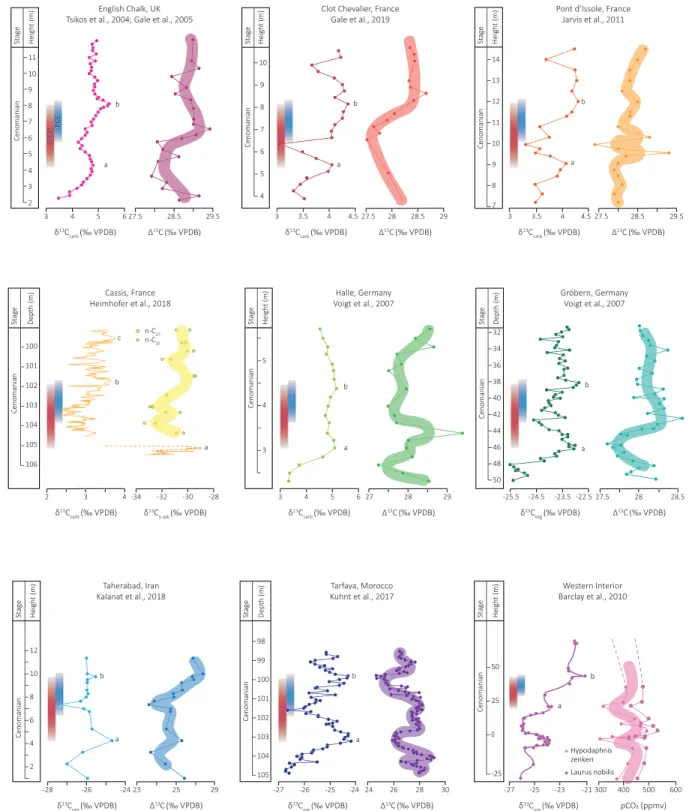
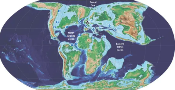
Figure 3. Global distribution of known records demonstrating the Plenus CIE (a negativeδ13C excursion between points“a” and “b” in Figure 1) or an excursion in CO2across the Plenus interval, as indicated byΔ13C, compound‐ specific δ13C, or leaf stomata. 1 Pratt's landing (van Helmond et al., 2016); Vermillion River, Well 10–35‐45‐2WA (Prokoph et al., 2013). 2 Cuba, KS (Bowman & Bralower, 2005); Pueblo (Barclay et al., 2010; Bowman & Bralower, 2005; Caron et al., 2006; Keller et al., 2008; Pratt, 1985; Sageman et al., 2006); USGS Portland‐1 core (Eldrett et al., 2017); Aristocrat Angus core (Joo & Sageman, 2014); Hot Springs, CO (Desmares et al., 2007); SH#1 core (Jones et al., 2019); generalized Western Interior Seaway (Orth et al., 1993). 3 Great Valley sequence, CA (Du Vivier et al., 2015). 4 Innes‐1 core, Iona‐1 core, Well X core (Eldrett et al., 2017). 5 Axaxacoalco, Barranca el Tigre, Barranco el Canon (Elrick et al., 2009). 6 Laurichocha, Piedra Parada, Uchucchacua (Navarro‐Ramirez et al., 2016, 2017). 7 Bass River, NJ (Bowman & Bralower, 2005; van Helmond et al., 2013). 8 ODP Site 1258 (Erbacher et al., 2005); ODP Site 1260 (Eldrett et al., 2017; Erbacher et al., 2005; Forster et al., 2007: Van Bentum et al., 2012); ODP Site 1261 (Eldrett et al., 2017; Erbacher et al., 2005). 9 DSDP Site 367 (Dickson et al., 2016; Forster et al., 2007; Kuypers et al., 1999; Sinninghe Damsté et al., 2008). 10 Tarfaya (Keller et al., 2008; Kolonic et al., 2005; Kuhnt et al., 2017; Kuypers et al., 2002; Tsikos et al., 2004); Mpl, S57, S75 (Kolonic et al., 2005); S13 (Kolonic et al., 2005; Kuypers et al., 1999). 11 ODP Site 1276 (Sinninghe Damsté et al., 2008; van Helmond et al., 2014). 12 Arobes, Ganuza, Menoyo (Kaiho et al., 2014); Manilvala (Mort et al., 2007); Puentedey (Barroso‐Barcenilla et al., 2011). 13 Dover (this study; Jeans et al., 1991; Lamolda et al., 1994); Eastbourne (Gale et al., 2005; Jenkyns et al., 1994; Paul et al., 1999; Pearce et al., 2009; Tsikos et al., 2004; Zheng et al., 2013); Culver cliff (Jarvis et al., 2001). 14 Gröbern (Voigt et al., 2006); Halle (Voigt et al., 2007); Wunstorf (Du Vivier et al., 2014; Voigt et al., 2008); Roter Sattel (Charbonnier et al., 2018). 15 Lambruisse (Takashima et al., 2009); Pont d'Issole (Grosheny et al., 2006; Jarvis et al., 2011); Les Lattes, Le Bourgeut (Grosheny et al., 2017); Cassis (Heimhofer et al., 2018); Clot Chevalier (Gale et al., 2019). 16 Pecínov, Czech Republic (Košťák et al., 2018). 17 Bottaccione (Kuroda et al., 2007); Furlo (Mort et al., 2007); Gubbio (Jenkyns et al., 1994; Tsikos et al., 2004); Raia del Pedale (Owens et al., 2013); Monte Coccovello, Monte Varchera (Parente et al., 2008). 18 Crimea (Fisher et al., 2005). 19 Jerissa (Zaghbib‐Turki & Soua, 2013); Oued Mellegue (Nederbragt & Fiorentino, 1999); Wadi Bahoul (Caron et al., 2006). 20 Wadi Feiran (El‐Sabbagh et al., 2011). 21 Ghawr Al Mazar (Wendler et al., 2016); Wadi Karak (Farouk et al., 2017). 22 Aimaki, Khadzhalmakhi, Levashi (Gavrilov et al., 2013). 23 Taherabad (Kalanat et al., 2018). 24 Tappu (Nemoto & Hasegawa, 2011); Yezo (Du Vivier et al., 2015). 25 ODP Site 530 (Forster et al., 2008). 26 Gongzha (Bomou et al., 2013); Tingri (Li et al., 2006). 27 Sawpit Gully, Mangaotane B (Gangl et al., 2019; Hasegawa et al., 2013); Mangaotane A (Hasegawa et al., 2013). Base map from Scotese, (2014).
10.1029/2019PA003631
in pCO2. Leaf‐wax δ13C records from the Cenomanian–Turonian organic‐
rich sediments from the equatorial Atlantic (Kuypers et al., 1999; Sinninghe Damsté et al., 2010) and France (Heimhofer et al., 2018) sug-gest a rise in CO2from point“a” to the trough of the P‐CIE and then a fall
to point“b” (Figure 5). Given the similarity in CO2trends indicated by
these two independent proxies for atmospheric CO2, we suggest that the
rise in pCO2from point“a” and fall across point “b” likely reflect global
changes in the atmosphere. Δ13C (the offset between δ13C
carb and δ13Corg in marine sediments)
reflects the degree of carbon fractionation during photosynthesis, which is pCO2‐dependent (Farquhar et al., 1989; Freeman & Hayes, 1992).
Δ13
C records changes in dissolved seawater CO2concentration, which is
assumed to be in equilibrium with atmospheric CO2, and thus can be used
as a pCO2proxy.Δ13C marine records from the UK, France, Germany,
and Morocco show a similar trend to the terrestrial records from the Western Interior Seaway: namely, a rise then fall in CO2over the P‐CIE
interval (Gale et al., 2005; Jarvis et al., 2011; Voigt et al., 2006, 2007). Two Δ13C records, from France (Gale et al., 2019) and Iran (Kalanat et al., 2018), show different trends: both indicate an increase in pCO2over
the P‐CIE, although both show poorly resolved Plenus CIEs owing to con-densation, diagenesis, or poorly resolved stratigraphy.
Despite their general agreement with the terrestrial proxies for pCO2,
Δ13C records must be treated with some caution when interpreted in the
context of atmospheric CO2changes. Changes in oceanography may have generated local variations in
ocean CO2fluxes and concentrations. For example, the incursion of a cold, oxygenated water mass across
a region would have led to the remineralization of buried organic matter, causing a localized increase in [CO2] in bottom waters and potentially, particularly in areas of upwelling, to CO2outgassing to the
atmo-sphere. As the total organic carbon (TOC) content of strata varied regionally, the degree of remineralization would have varied between sites, producing different CO2 concentrations in different locations.
Furthermore, as CO2solubility is dependent on water temperature (e.g., Broecker & Peng, 1974), a cold
water mass would contain higher concentrations of dissolved CO2compared with warmer waters, and this
alone would have affected the local pH without involving any atmospheric processes. Euxinic conditions may also affect local CO2concentrations, as the degradation of organic matter allows phosphate to be
released back to bottom waters, driving increased productivity and organic‐matter deposition (Jarvis et al., 2011; Mort et al., 2007). These local processes could potentially mask any signal of atmospheric pCO2change
and, if not recognized, could lead to erroneous interpretations of the drivers of the PCE. 4.2. Evidence for Changing Temperature
The Plenus Cold Event wasfirst recognized based on the southerly migration of boreal fauna coincident with two positiveδ18O excursions in the Chalk of Dover, UK (Gale & Christensen, 1996; Jefferies, 1962). In the Dover Chalk records, cooling is observed in Beds 2 and 4–8 of the Plenus Marls (Figures 1 and 2), supported by numerous other records of faunal assemblages andδ18O from southeast England, with some variation in the timing of the onset of cooling (this study; Gale et al., 2005; Jeans et al., 1991; Jefferies, 1962, 1963; Lamolda et al., 1994; Paul et al., 1999; Tsikos et al., 2004; Voigt et al., 2004, 2006). The main phase of cooling in south-east England, as exemplified by the carbon‐isotope record, extends from the trough of the P‐CIE to point “b”. The early stages of OAE 2 have been studied extensively across the Northern Hemisphere, with multiple quantitative and qualitative records indicating brief cooling around the P‐CIE interval (Figure 6). δ18O
(Kalanat et al., 2018; Kuhnt et al., 2017), TEX86(Forster et al., 2007; Sinninghe Damsté et al., 2010), faunal
assemblages (Eldrett et al., 2017; van Helmond et al., 2013, 2016), and foraminiferal coiling direction (Desmares et al., 2016) show clear evidence for cooling across the Tethyan margins, North Atlantic, and Western Interior Seaway. In France and Germany, incursions of boreal fauna and dinocysts also indicate cooling, as supported byδ18O and TEX86 records (Figure 7; Takashima et al., 2009; Voigt et al., 2006,
Figure 4. Comparison ofδ13Corgandδ13Chopanerecords from ODP Site
1276, Cape Verde Basin (adapted from Sinninghe Damsté et al., 2010) demonstrating a stratigraphic offset in the position of the negative excursion seen inδ13Corgat ~1,083.1 m below seafloor and in δ13Chopaneat
2007, 2008; van Helmond et al., 2015). However, some bulk δ18O records from hemipelagic clay‐rich carbonates (e.g., Pont d'Issole, Vocontian Basin, France) show no clear excursion across the PCE interval (Jarvis et al., 2011; Voigt et al., 2006), even though nearby sections, a few tens of kilometers away, show dis-tinct positive excursions of 1–1.5‰ locally alongside qualitative measures of cooling, such as changes in the direction of foraminiferal coiling (Gale et al., 2019; Grosheny et al., 2017).
Figure 5. Records of CO2change across the Plenus interval. The red bands indicate the P‐CIE, and the blue bands indicate the PCE in a strict sense; points “a” to
“c” of the OAE are labeled. Colored bands illustrate visual approximations of trends.
10.1029/2019PA003631
Although cooling appears to be geographically widespread, the precise timing of the falls in local paleotem-perature is not consistent globally, or even within a single basin. For example, in Germany, Pueblo and DSDP Site 367, cooling starts well before the P‐CIE and reaches its lowest temperature around point “a,” based on TEX86,δ18O, foraminiferal coiling, and faunal assemblages (Figure 7; Voigt et al., 2007; Forster
et al., 2007; van Helmond et al., 2015; Desmares et al., 2016). By contrast, in the Chalk records from southern England, and TEX86records from DSDP Site 367 (equatorial Atlantic) and ODP Site 1276 (North Atlantic),
the cooling apparently started later and peaked around point“b” (Forster et al., 2007; Gale & Christensen, 1996; Lamolda et al., 1994; Sinninghe Damsté et al., 2010). Other sites, such as Tarfaya and ODP Site 1260, suggest a more complex pattern of cooling, with multiple excursions in the TEX86andδ18O records
(Forster et al., 2007; Kuhnt et al., 2017). However, Tarfaya is recognized as a paleo‐upwelling area, which would have complicated the SST response (e.g., Einsele & Wiedmann, 1982; Kolonic et al., 2005). Although local diagenesis may have affected some of the SST records, in particular those deriving from oxy-gen isotopes, the existence of consistent differences in the relative timing between carbon‐isotope events and local paleotemperature minima (based on both geochemical and paleontological proxies) suggests that the cooling of water masses was diachronous.
4.3. Evidence for Changing Water Mass Character
Geochemical, lithological, and faunal records across OAE 2 demonstrate significant and variable changes in water mass character associated with the event, variously attributed to changes in redox, circulation, and/or volcanic activity (Figure 8; e.g., Eicher & Worstell, 1970; Orth et al., 1993; MacLeod et al., 2008; Martin et al., 2012; Thomas & Tilghman, 2014). However, few records are of sufficiently high resolution to both identify the Plenus interval and any oceanographic changes associated therewith and determine the precise cause of these changes.
Figure 6. Global distribution of known records demonstrating a change in temperature across the PCE interval, based on records of TEX86,δ18O, faunal assemblages, and foraminiferal coiling. 1 Pratt's Landing (van Helmond et al., 2016). 2
Hot Springs, SD (Desmares et al., 2016); Pueblo (Caron et al., 2006; Desmares et al., 2016); USGS Portland‐1 Core (Eldrett et al., 2017). 3 Iona‐1 core, Innes‐1 core, Well X core (Eldrett et al., 2017). 4 Bass River, NJ (van Helmond et al., 2013). 5 ODP site 1260 (Eldrett et al., 2017; Forster et al., 2007). 6 DSDP Site 367 (Forster et al., 2007). 7 Tarfaya (Kuhnt et al., 2017; Tsikos et al., 2004). 8 ODP Site 1276 (Sinninghe Damsté et al., 2008). 9 Arobes, Ganuza, Menoyo (Kaiho et al., 2014); Puentedey (Barroso‐Barcenilla et al., 2011). 10 Dover (this study; Jefferies, 1962; Jeans et al., 1991; Lamolda et al., 1994); Eastbourne (Jenkyns et al., 1994; Paul et al., 1999; Pearce et al., 2009; Tsikos et al., 2004; Voigt et al., 2004, 2006; Zheng et al., 2013). 11 Gröbern (Voigt et al., 2006); Halle (Voigt et al., 2007); Wunstorf (van Helmond et al., 2015). 12 Cassis (Heimhofer et al., 2018); Clot Chevalier (Gale et al., 2019); Lambruisse (Takashima et al., 2009); Les Lattes (Gale & Christensen, 1996); Pont d'Issole (Jarvis et al., 2011). 13 Gubbio (Jenkyns et al., 1994). 14 Crimea (Fisher et al., 2005). 15 Oued Mellegue (Nederbragt & Fiorentino, 1999); Wadi Bahoul (Caron et al., 2006). 16 Wadi Karak (Farouk et al., 2017). 17 Amaki, Khadzhalmakhi, Levashi (Gavrilov et al., 2013). 18 Taherabad (Kalanat et al., 2018). Base map from Scotese, (2014).
Chromium is a redox‐sensitive metal that may also be derived from basalt–seawater interactions, and as such is a useful tool for tracking changes in seawater chemistry (e.g., Bonnand et al., 2013; Holmden et al., 2016; Remmelzwaal et al., 2019). At Dover in SW England, carbonate‐fraction Cr concentrations show an approximatelyfivefold increase over the uppermost marls (this study; Figure 2). Similar spikes
Figure 7. Records of SSTs during the Plenus interval. The red bands indicate the P‐CIE, and the blue bands indicate the PCE in a strict sense; points “a” to “c” of the OAE are labeled. Dover stratigraphy from Lamolda et al. (1994); Wunstorf stratigraphy from Voigt et al. (2008). Colored bands illustrate visual approximations of trends.
10.1029/2019PA003631
in geochemical species (such as Cr, Mo, U, Mn) have been recorded at sites in the Chalk Sea and/or along the Tethyan margins (e.g., Orth et al., 1993; Jarvis et al., 2001; Kolonic et al., 2005; Pearce et al., 2009; Jenkyns et al., 2017; Charbonnier et al., 2018; Clarkson et al., 2018; Danzelle et al., 2018; Sweere et al., 2018; Gale et al., 2019), North Atlantic (Dickson et al., 2016; Eldrett et al., 2017; van Helmond et al., 2014), and the Western Interior Seaway (Eldrett et al., 2017; Holmden et al., 2016; Orth et al., 1993). These excursions have been attributed to a period of increased bottom‐water oxygenation during which the remineralization of organic matter either released trace metals into the water column and/or removed anoxic/euxinic sinks for hydrothermally enriched bottom waters (Jenkyns et al., 2017). However, some sites show excursions in certain geochemical species but not others (e.g., Danzelle et al., 2018; Eldrett et al., 2017; Owens et al., 2013; Sweere et al., 2018). These differences may be due to the different reduction potentials of various elements and the local redox conditions pertaining at any one site. Local redox conditions during the Plenus interval may have prevented certain elements from being enriched in discrete reduced phases, such as in sulfides, or substituting in pyrite or
Figure 8. Global distribution of known records demonstrating a change in water mass character across the Plenus inter-val, as indicated by elemental, isotopic, lithological, or faunal changes in the sedimentary record. 1 Vermillion River (Prokoph et al., 2013). 2 Angus Aristocrat core (Zhou et al., 2015); Cuba, KS (Bowman & Bralower, 2005; Eldrett et al., 2014); Hot Springs, SD (Desmares et al., 2016); USGS Portland‐1 core (Du Vivier et al., 2014; Eldrett et al., 2017; Holmden et al., 2016); generalized Western Interior Seaway (Orth et al., 1993); Pueblo (Bowman & Bralower, 2005; Caron et al., 2006; Keller et al., 2008; Elderbak et al., 2014). 3 Great Valley sequence, CA (Du Vivier et al., 2015). 4 Innes‐1 core, Iona‐1 core, Well X core (Eldrett et al., 2017). 5 Barranco el Canon (Elrick et al., 2009; Sweere et al., 2018). 6 Bass River, NJ (Bowman & Bralower, 2005). 7 ODP Site 1258 (Erbacher et al., 2005; Friedrich et al., 2006; Ostrander et al., 2017; Zhou et al., 2015); ODP Site 1260 (Du Vivier et al., 2014; Eldrett et al., 2017; Erbacher et al., 2005; Forster et al., 2007; Friedrich et al., 2006; Turgeon & Creaser, 2008); ODP Site 1261 (Erbacher et al., 2005; Friedrich et al., 2006). 8 DSDP Site 367 (Kuypers et al., 1999; Forster et al., 2007, 2008; Sinninghe Damsté et al., 2008; Du Vivier et al., 2014; Dickson et al., 2016). 9 Tarfaya (Dickson et al., 2016; Keller et al., 2008; Kuhnt et al., 2017; Kuypers et al., 2002; Tsikos et al., 2004); Mpl, S13, S57, S75 (Kolonic et al., 2005). 10 ODP Site 1276 (Sinninghe Damsté et al., 2008; van Helmond et al., 2014). 11 Puentedey (Barroso‐Barcenilla et al., 2011); Arobes (Kaiho et al., 2014); Ganuza (Kaiho et al., 2014; Peryt & Lamolda, 1996); Manivala (Mort et al., 2007); Menoyo (Kaiho et al., 2014; Peryt & Lamolda, 1996). 12 Dover (this study; Jeans et al., 1991); Eastbourne (Clarkson et al., 2018; Lu et al., 2010; Orth et al., 1993; Owens et al., 2013; Paul et al., 1999; Pearce et al., 2009; Sweere et al., 2018; Zheng et al., 2013; Zhou et al., 2015). 13 Wunstorf (van Helmond et al., 2015); Halle (Voigt et al., 2007); Roter Sattel (Charbonnier et al., 2018); Wunstorf (Du Vivier et al., 2014; van Helmond et al., 2015). 14 Clot Chevalier (Gale et al., 2019); Lambruisse (Takashima et al., 2009); Le Bourgeut (Grosheny et al., 2017); Pont d'Issole (Danzelle et al., 2018; Grosheny et al., 2006; Jarvis et al., 2011); Vocontian Basin (Du Vivier et al., 2014). 15 Bottaccione (Kuroda et al., 2007); Furlo (Mort et al., 2007); Gubbio (Tsikos et al., 2004); Raia del Pedale (Clarkson et al., 2018; Owens et al., 2013; Sweere et al., 2018; Zhou et al., 2015). 16 Crimea (Fisher et al., 2005). 17 Oued Mellegue (Nederbragt & Fiorentino, 1999); Wadi Bahoul (Caron et al., 2006). 18 Wadi Feiran (El‐Sabbagh et al., 2011). 19 Wadi Karak (Farouk et al., 2017). 20 Aimaki, Khadzhalmakhi, Levashi (Gavrilov et al., 2013). 21 Gharesu (Kalanat et al., 2016); Taherabad (Kalanat et al., 2016, 2017). 22 Tappu (Nemoto & Hasegawa, 2011); Yezo group (Du Vivier et al., 2015). 23 DSDP Site 530 (Du Vivier et al., 2014; Forster et al., 2008). 24 Gongzha (Bomou et al., 2013). Base map from Scotese, (2014).
adsorbed onto organic matter but not allowed them to be incorporated in carbonates in more oxidized form even if present in relative abundance in seawater. Regardless of the cause, these variable expressions of redox change across the Plenus interval make it difficult to deconvolve global from local drivers of paleoenvironmental change.
Neodymium‐isotope ratios, expressed as εNd, are a powerful tool for reconstructing changes in past ocean
cir-culation (Frank, 2002; Goldstein & Hemming, 2003). Roughly coeval with the Cr excursion in the Chalk of SW England, large (~1.5ε unit) excursions in neodymium isotopes across the PCE interval suggest changing circulation and/or possible input of magmatically derived radiogenic Nd (this study; Zheng et al., 2013, 2016). A link has been drawn between LIPs and oceanic anoxic events, particularly with respect to the Caribbean and High Arctic Large Igneous Provinces as possible triggers for OAE 2 (e.g., Snow et al., 2005; Tegner et al., 2011; Zheng et al., 2013). Osmium‐isotope records from across the world have identified per-iods of volcanism or some form of basalt–seawater interaction around the Cenomanian–Turonian boundary, indicating likely LIP activity immediately prior to the onset of OAE 2 (Du Vivier et al., 2014, 2015; Scaife et al., 2017; Schröder‐Adams et al., 2019; Turgeon & Creaser, 2008). Basalt–seawater interactions would not have just affected seawater Nd and Os but also other trace metals and isotopes, which further compli-cates the interpretation of their sedimentary records.
Ce anomalies reflect the oxidation state of seawater through the oxidation of Ce (III) to insoluble and particle‐reactive Ce (IV) (De Baar et al., 1988; Zhou et al., 2015; Remmelzwaal et al., 2019). In the Dover record, Ce* steadily decreases upsection, mirroring the generally increasing pattern ofδ13C. These data can be compared with trace‐element data from the Eastbourne section (Jenkyns et al., 2017; Lu et al., 2010). Cerium anomalies at Dover are generally lower during the PCE than prior to the event, but there is a significant increase in Ce/Ce* from 0.7 to 0.83 at the beginning of the OAE event in the Dover section. This rise is consistent with Mn/Ca data for the Eastbourne section, suggestive of an initial move to a less oxic subseafloor, whereas the overall decrease in Ce/Ce*, particularly during the PCE, is consistent with I/Ca ratios indicating a move to more oxic surface waters at this time (Lu et al., 2010). Seawater and carbo-nates in modern marine environments commonly have both Ce and La anomalies and this is best demon-strated by calculating Ce/Ce* and Pr/Pr* values, which also covary with each other (Webb & Kamber, 2000). Our new carbonate record indicates that the late Cenomanian seawater also has both Ce and La anomalies. While Ce/Ce* and Pr/Pr* (supp. info.) values vary smoothly through the section, they are prin-cipally indicative of variable redox conditions, whereas La/Pr ratios still retain information about source input and are much more variable. In this case, the La/Pr ratio is a useful guide to the amount of basaltic input to the seawater because average altered basaltic crust has La/Pr value of 1.65 (Kelley et al., 2003), whereas the upper continental crust has a value of 4.37 (Rudnick & Gao, 2003). Therefore, lower La/Pr ratios are indicative of an increased basaltic input, either from basalt–seawater interaction or re‐ oxygenation of seafloor sediment. La/Pr ratios decrease at the beginning of the OAE level and during the interval of the two cooling events, particularly the main PCE, at which level it is consistent with positive shifts in Nd isotopes.
Re‐oxygenation of bottom water has also been invoked as the cause of decreased TOC in Plenus records from the Tethys, North Atlantic, and even Japan (Bowman & Bralower, 2005; Dickson et al., 2016; Eldrett et al., 2014, 2017; Forster et al., 2007; Jarvis et al., 2011; Kuhnt et al., 2017; Nemoto & Hasegawa, 2011; Sinninghe Damsté et al., 2010; Tsikos et al., 2004; van Helmond et al., 2013, 2014). However, many sites record no change in the TOC, or in some cases an increase, suggesting locally sustained bottom‐water oxygenation or simply changes in productivity (e.g., Dickson et al., 2016; Gavrilov et al., 2013; Kolonic et al., 2005; Kuhnt et al., 2017; Kuypers et al., 2002; Mort et al., 2007; Tsikos et al., 2004).
Faunal records showing an increase in benthic organisms and bioturbation during the Plenus interval sug-gest increased bottom‐water oxygenation at sites across the Chalk Sea of northern Europe (Jarvis et al., 1988; Paul et al., 1999; Peryt & Lamolda, 1996; Takashima et al., 2009), Tethyan margin (Barroso‐Barcenilla et al., 2011; Kalanat et al., 2016), North Atlantic (Eldrett et al., 2017), and Western Interior Seaway (Desmares et al., 2007; Elderbak et al., 2014). However, as with the TOC records, some sites show no change in benthic faunal abundance over this interval, or in some cases a decrease, further suggesting locally sustained bottom‐ water anoxia (e.g., El‐Sabbagh et al., 2011; Friedrich et al., 2006; Grosheny et al., 2006, 2017; Keller et al., 2008).
10.1029/2019PA003631
Trace‐metal, isotope, TOC, and faunal records all suggest pockets of re‐oxygenation, but it remains difficult to link these directly to global changes in the carbon cycle or temperature. Furthermore, different water depths at different sites will have directly influenced bottom‐water oxygenation, and may determine whether anoxia could have occurred in thefirst place.
5. Implications for Understanding Environmental Changes During the Plenus
Cold Event
5.1. Carbon‐Cycle Perturbation
The remarkable consistency of the carbon‐isotope signature of OAE 2 across the globe allows for chemostra-tigraphic correlation of the event, albeit with the caveat that variable organic‐matter sources can affect bulk δ13C
organd variable diagenesis can affectδ13Ccarb, particularly in sediments containing potentially reactive
organic matter.
In a comparison of biostratigraphy and chemostratigraphy of OAE 2 between Europe and North America, Gale et al. (1993) found a consistent relationship between the two, which these authors took as evidence for effective synchroneity between certain paleontological markers and the carbon‐isotope events in Europe and North America (despite some endemism and preservation problems, particularly associated with facies changes). More recent and higher‐resolution studies support this contention, namely, global par-allels in the general patterns of microfossil and macrofossil biostratigraphy andδ13C correlations (Jarvis et al., 2006; Wendler, 2013). These records indicate a globally synchronous response of the biostratigraphic and chemostratigraphic record to the OAE, and that the characteristic carbon‐isotope signature can be reli-ably used in correlation.
The terrestrially derived CO2records and the majority of marine CO2records show a rise then fall in
atmo-spheric CO2across the P‐CIE, suggesting a global carbon‐cycle event. As such, we propose that the negative
δ13C excursion could—and should—be used as a stratigraphic marker to identify the Plenus interval in local
archives. This approach to stratigraphic correlation avoids potential miscorrelation issues caused by possible diachroneity of any cooling observed at different locations, which could have been impacted by the local oceanographic conditions.
The driver of this CO2change is more difficult to identify. Initially, it was proposed that increased organic‐
carbon burial during the initial stages of OAE 2 drove a drawdown of atmospheric CO2(Arthur et al., 1988;
Forster et al., 2007; Freeman & Hayes, 1992; Jarvis et al., 2011; Jenkyns et al., 1994; Kuypers et al., 1999; Sinninghe Damsté et al., 2010). Therefore, an increase in bottom‐water re‐oxygenation during the Plenus interval would have led to a temporary reduction of organic‐matter deposition and/or the remineralization of sedimentary carbon on the seafloor, driving an increase in CO2. The Cenomanian–Turonian boundary
was also a period of enhanced basalt–seawater interaction owing to the emplacement of at least two large igneous provinces (LIPs): the Caribbean Large Igneous Province (CLIP; Snow et al., 2005) and the High Arctic Large Igneous Province (HALIP; Tegner et al., 2011; Davis et al., 2016; Kingsbury et al., 2018; Schröder‐Adams et al., 2019). A cessation of this volcanic outgassing may have resulted in an overall decrease in pCO2(e.g., Du Vivier et al., 2014, 2015; Scaife et al., 2017; Turgeon & Creaser, 2008). Indeed,
Kuroda et al. (2007) suggested, based on a coeval shift in Pb isotopes indicative of an increase in hydrother-mal input of Pb, that the negative carbon‐isotope excursion observed during the Plenus interval reflects an increase in pCO2due to volcanism, rather than a drop in global burial rates of organic carbon. The changing
balance between CO2drawdown due to organic‐carbon burial versus volcanic and tectonic emissions of this
greenhouse gas is difficult to constrain. However, a rise in atmospheric CO2would drive an increase in
glo-bal temperatures—the opposite of what is observed. This apparent mismatch between theory and observa-tion highlights complicaobserva-tions in drawing causative links between putative CO2levels and the PCE, as it
was originally interpreted.
5.2. Accompanying Climatic Phenomena
There is a wealth of data indicating widespread paleoenvironmental change during the early stages of OAE 2 but the question remains as to what drove such phenomena in different parts of the globe. Accounting for problems inherent in biostratigraphic, chemostratigraphic, and lithostratigraphic correlation, the records show little consistency in the timing of temperature and seawater chemistry (Figures 5 and 7). The onset
of these changes apparently appeared much earlier at some sites than others, even locally preceding the negative carbon‐isotope excursion, suggesting that oceanic processes may have responded to forcing mechanisms other than just changes in ocean–atmosphere pCO2, such as a change in local circulation,
pro-ductivity, or basalt–seawater interactions. 5.2.1. Changing Water Mass Character
A change in circulation, bottom‐water re‐oxygenation, and basalt–seawater interactions have variously been proposed to drive the excursions seen in different proxy records discussed in section 4.3. However, records of seawater chemistry are difficult to interpret as the proxies may have responded to more than one process, or one process may have driven another. The neodymium‐isotopic signal of a water mass may reflect changes in circulation, but it can also be affected by basalt–seawater interaction introducing radiogenic Nd. Although complicating the interpretation ofεNdrecords, the geochemical imprint of basalt on seawater may be helpful
for tracing the source of a water mass to volcanically affected areas.
The positiveεNdexcursion in the Eastbourne record was interpreted by Zheng et al. (2016) to reflect the input
of strongly radiogenic Nd from volcanism through relatively oxygen‐poor water, citing the coeval emplace-ment of the Caribbean Large Igneous Province (Snow et al., 2005) and the High Arctic Large Igneous Province (Davis et al., 2016; Kingsbury et al., 2018; Tegner et al., 2011). Due to the lack of outcrop, the chem-istry and eruption history of these LIPs are poorly constrained, which makes it difficult to pinpoint the source of any volcanically derived radiogenic Nd. For CLIP to have acted as the source of radiogenic Nd would have required transfer of the geochemical bottom‐water signal from the Pacific Ocean to southern England across the eastern paleo‐Pacific and proto‐Atlantic (cf. Trabucho‐Alexandre, 2014). Given that the residence time of neodymium in the ocean today is roughly equal to the mixing time of the ocean (Frank, 2002; Goldstein & Hemming, 2003; Thomas, 2005), CLIP‐derived radiogenic Nd is unlikely to have induced such a large positive shift inεNdin such a distal location as southern England. Neodymium might
have had a longer residence time in relatively deoxygenated seawater because Fe‐Mn oxyhydroxides (a sink for Nd) would not have been stable under such conditions (Halliday et al., 1992); however, such conditions would have been less applicable during the apparently more oxygenated conditions (at least in southern England) of the PCE itself. If a water mass from the vicinity of the HALIP moved south, carrying a radiogenic Nd signature, it could have produced a positiveεNdexcursion while simultaneously causing a drop in water
temperature, as seen in the Dover record (Figure 2). Furthermore, as O2solubility is dependent on water
temperature (e.g., Broecker & Peng, 1974), a cold water mass would have contained higher concentrations of dissolved O2compared with warmer waters and could have induced a redox shift in bottom waters, as
sug-gested by the trace‐metal record at Dover (Figure 2) and Eastbourne (Jenkyns et al., 2017).
Trace‐metal and isotopic excursions have been ascribed to two factors: (1) bottom‐water re‐oxygenation dur-ing the PCE, whereby the remineralization of trace‐metal‐rich organic matter deposited durdur-ing the early stages of the OAE released metals into the water column, some of which were subsequently incorporated into nannofossil and foraminiferal carbonate (Jenkyns et al., 2017), and (2) alternatively, or additionally, the transient loss of the organic‐rich sink during re‐oxygenation events during the Plenus interval, with ongoing basalt–seawater interaction continuing to liberate volcanically derived trace metals, allowed their buildup in ocean waters (Orth et al., 1993; Pearce et al., 2009; Holmden et al., 2016; Jenkyns et al., 2017). Decreased TOC across the Plenus interval has also been suggested to indicate a redox shift (e.g., Eldrett et al., 2014, 2017; Jarvis et al., 2011; Tsikos et al., 2004), although organic‐matter content may be affected by changes in preservation, productivity, or dilution. Increased oxygenation of bottom waters would inhibit the deposition of organic matter, although this assumes a simple coupling between anoxia and organic‐ matter deposition in thefirst place, which is manifestly a gross simplification (e.g., Demaison & Moore, 1980; Pedersen & Calvert, 1990). Deposition of the characteristic black shales of OAE 2 was not a global phe-nomenon, but rather limited to environments that favorably supported organic‐matter burial, particularly the Atlantic and Tethyan regions and the equatorial Pacific (Schlanger et al., 1987; Takashima et al., 2009). Furthermore, local to regional variations in productivity, preservation, sedimentation rate, and sea-water chemistry led to differences in the timing of local maxima in organic‐carbon burial rates. Particularly in former upwelling areas, such as the western sides of continents or the paleo‐equator, increases in organic productivity, initially unrelated to bottom‐water or midwater redox, may have driven
10.1029/2019PA003631
an increase in organic‐matter deposition. An increased supply of biologically significant metals or minerals may also have resulted directly from basalt–seawater interactions, and/or increased terrestrial weathering, and consequent accelerated fluvial nutrient input to the oceans, which may in turn have driven an expansion of organic productivity (Jenkyns, 2010). Local changes in these processes—whether related or unrelated to global CO2and temperature—may have driven either an increase or decrease in organic‐
matter deposition that might be misconstrued as a redox shift. These factors may also explain the records of increased TOC across the Plenus interval in Spain (Mort et al., 2007) and Morocco (Kuhnt et al., 2017). Given the enhanced hydrological cycle, proposed to have driven an increase in silicate weathering during the OAE (Blättler et al., 2011; Pogge von Strandmann et al., 2013), changes in terrestrial weathering and sedi-mentary dilution may also have affected the TOC without changing productivity or preservation.
5.2.2. Cooling
Cooling events are observed across the Northern Hemisphere during the Plenus interval, for which a range of mechanisms has been proposed.
1. A causal link has been suggested between SSTs and the carbon cycle during OAE 2: at its simplest, the widespread deposition of organic matter during OAE 2 is credited with leading to CO2drawdown and,
in turn, transient cooling (Arthur et al., 1988; Forster et al., 2007; Freeman & Hayes, 1992; Jarvis et al., 2011; Jenkyns et al., 1994; Kuypers et al., 1999; Sinninghe Damsté et al., 2010). However, if these tem-perature records (TEX86,δ18O, fauna) were solely recording the SST response to global atmospheric
cool-ing, they would be expected to show a degree of synchroneity and expression: cooling occurring during and afterthe CO2decrease, during the later phase of the P‐CIE close to point “b” (e.g., scenario (1) in
Figure 9. Potential models for cooling during the PCE.δ13C from Eastbourne (Tsikos et al., 2004). The gray box indicates the OAE 2 interval and the red band indicates the P‐CIE; points “a” to “d” of the δ13C curve are labeled. The red lines indicate CO2, the blue lines indicate SST, and the green line indicates circulation. Values are arbitrary. Model (1): A direct
link between CO2, atmospheric temperatures, and SSTs would produce a cooling interval after a drop in CO2. Model (2): A
fall in CO2would drive global temperature decrease, forcing a circulation change and, in turn, further cooling. In this
model, cooling must come after the CO2change. Model (3): No direct link between CO2and SSTs would produce variable
Figure 9; Eastbourne and ODP Site 1276 in Figure 7). While a global decrease in temperatures would have been a necessary response to falling atmospheric CO2levels, the SST records—if accepted at face
value—show significant variability in the timing of the cooling relative to the P‐CIE. The TEX86,δ18O,
and faunal records that show cooling preceding the CO2decrease, in the early phase of the P‐CIE close
to point“a” (e.g., Wunstorf, Gröbern, Bass River, Pueblo; Figure 7), which implies either an indirect response of local SSTs to CO2change, or simply the effect of local oceanographic conditions independent
of global change. Furthermore, it is difficult to directly link the cooling seen at point “b” to global pro-cesses, when the drop in temperature may have been due to a circulation change bringing cooler water to a locality (as seen by the simultaneous cooling and Nd excursion in SE England; Figures 2 and 9). 2. Ocean circulation is thought to have been a critical component of the climate system during the Plenus
interval, wherein CO2drawdown led to global cooling and increased latitudinal temperature gradients,
which in turn drove a change in circulation (Eldrett et al., 2017; van Helmond et al., 2014; Zheng et al., 2013). However, there are two problems with this hypothesis. Firstly, as in (1), this model does not account for cooling preceding the CO2decrease. Secondly, if global cooling drove the circulation
change, one would expect one phase of cooling after the CO2change then another after the circulation
change, but none of the records show this. As such, this model cannot account for cooling in the early phase of the P‐CIE, close to point “a,” which indicates that CO2‐driven circulation change was not a
direct driver of the cooling at all sites.
3. Alternatively, circulation might have been altered due to factors unrelated to global temperatures and latitudinal gradients, perhaps owing to changes in upwelling (e.g., Einsele & Wiedmann, 1982; Kolonic et al., 2005), deepening and shallowing of local sea levels affecting upper ocean circulation patterns (e.g., Hancock, 1993; Voigt & Wiese, 2000; Voigt et al., 2006), or LIP‐related tectonics (e.g., Dostal & MacRae, 2018; Maher, 2001). These changes in circulation may have brought cooler water masses to regions bordering the Arctic, producing a decrease in local SSTs. Within the Chalk Sea and the Western Interior Seaway, rises inδ13C correlate with local transgressions (Voigt & Hillbrecht, 1997; Voigt & Wiese, 2000; Laurin et al., 2019). The timing of the cooling and circulation change observed in the Chalk Sea of southern England is coincident with the rising limb of the P‐CIE and evidence for a local transgression, suggesting that deepening of the sea may have allowed an ingress of cooler boreal waters. Although OAE 2 was a period of extreme global climate perturbation, the local temperature responses to increased CO2likely varied in magnitude, trend and, potentially, sign. Thus, interactions between climatic
and oceanographic processes may account for the different expressions of cooling seen at different sites, especially the cooling seen in the early stages of the P‐CIE. If nothing else, the apparent diachroneity in cool-ing highlights the problems associated with uscool-ing any local expression of temperature or water mass char-acter during the Plenus interval as a correlation tool or stratigraphic marker.
6. Conclusions
The Cenomanian–Turonian transition experienced extreme climate change and major volcanic and tectonic activity. The increase in silicate weathering due to an enhanced hydrological cycle on the continents and the weathering of LIP‐related basalts in the oceans probably drove a drawdown in CO2, as did high rates of
organic‐carbon burial. The ongoing basalt–seawater interaction, likely concentrated in the first half of OAE 2 based on regional osmium‐isotope signatures (Du Vivier et al., 2014, 2015), would have further affected both atmospheric pCO2and global carbon‐isotope compositions. By contrast, volcanic outgassing
and the cessation of organic‐carbon deposition would have driven an increase in pCO2. However, it is not
possible to disentangle these processes and their effects on the carbon cycle from the current data. During the Plenus interval, there is evidence for widespread environmental change across the Northern Hemisphere. The global extent of negativeδ13C excursions, coincident with records of increasing pCO2, suggest
an increase in atmospheric CO2and a global carbon‐cycle event—the Plenus CIE. However, the records of
cool-ing show no consistency in timcool-ing or expression, and suggest either that some or all of the proxy records are compromised by diagenesis or environmental factors, and/or there was no clear‐cut link between SSTs and atmospheric pCO2. While there was likely a global fall in temperatures relating to the drop in CO2, applying
simple cause‐and‐effect relationships between CO2 and temperature does not explain all observations.
Furthermore, variability in the timing and expression of changes in seawater chemistry, and problems in