The relevance of aerosol optical depth to cumulus fraction changes: a five-year climatology at the ACRF SGP site

(1)

HAL Id: hal-00303047

https://hal.archives-ouvertes.fr/hal-00303047

Submitted on 13 Aug 2007

HAL is a multi-disciplinary open access

archive for the deposit and dissemination of sci-entific research documents, whether they are pub-lished or not. The documents may come from teaching and research institutions in France or abroad, or from public or private research centers.

L’archive ouverte pluridisciplinaire HAL, est destinée au dépôt et à la diffusion de documents scientifiques de niveau recherche, publiés ou non, émanant des établissements d’enseignement et de recherche français ou étrangers, des laboratoires publics ou privés.

The relevance of aerosol optical depth to cumulus

fraction changes: a five-year climatology at the ACRF

SGP site

E. I. Kassianov, L. K. Berg, C. Flynn, S. Mcfarlane

To cite this version:

E. I. Kassianov, L. K. Berg, C. Flynn, S. Mcfarlane. The relevance of aerosol optical depth to cumulus fraction changes: a five-year climatology at the ACRF SGP site. Atmospheric Chemistry and Physics Discussions, European Geosciences Union, 2007, 7 (4), pp.11797-11837. �hal-00303047�

(2)

ACPD

7, 11797–11837, 2007

Relationships between aerosol optical depth and

cumulus fraction E. I. Kassianov et al. Title Page Abstract Introduction Conclusions References Tables Figures ◭ ◮ ◭ ◮ Back Close

Full Screen / Esc

Printer-friendly Version Interactive Discussion

Atmos. Chem. Phys. Discuss., 7, 11797–11837, 2007 www.atmos-chem-phys-discuss.net/7/11797/2007/ © Author(s) 2007. This work is licensed

under a Creative Commons License.

Atmospheric Chemistry and Physics Discussions

The relevance of aerosol optical depth to

cumulus fraction changes: a five-year

climatology at the ACRF SGP site

E. I. Kassianov, L. K. Berg, C. Flynn, and S. McFarlane

Pacific Northwest National Laboratory, 320 Q. Avenue, MSIN: K9-24, Richland, WA, 99352, USA

Received: 15 June 2007 – Accepted: 6 August 2007 – Published: 13 August 2007 Correspondence to: E. I. Kassianov (evgueni.kassianov@pnl.gov)

(3)

ACPD

7, 11797–11837, 2007

Full Screen / Esc

Printer-friendly Version Interactive Discussion Abstract

The objective of this study is to investigate, by observational means, the magnitude and sign of the actively discussed relationship between cloud fractionN and aerosol opti-cal depthτ_a. Collocated and coincident ground-based measurements and Terra/Aqua satellite observations at the Atmospheric Radiation Measurement (ARM) Climate

Re-5

search Facility (ACRF) Southern Great Plains (SGP) site form the basis of this study. The N−τ_a relationship occurred in a specific 5-year dataset of fair-weather cumulus (FWC) clouds and mostly non-absorbing aerosols. To reduce possible contamination of the aerosols on the cloud properties estimation (and vice versa), we use independent datasets ofτ_a andN obtained from the Multi-filter Rotating Shadowband Radiometer

10

(MFRSR) measurements and from the ARM Active Remotely Sensed Clouds Loca-tions (ARSCL) value-added product, respectively. Optical depth of the FWC cloudsτcld

and effective radius of cloud droplets re are obtained from the MODerate resolution

Imaging Spectroradiometer (MODIS) data.

We found that relationships between cloud properties (N,τcld, re) and aerosol

opti-15

cal depth are time-dependent (morning versus afternoon). Observed time-dependent changes of cloud properties, associated with aerosol loading, control the variability of surface radiative fluxes. In comparison with pristine clouds, the polluted clouds are more transparent in the afternoon due to smaller cloud fraction, smaller optical depth and larger droplets. As a result, the corresponding correlation between the surface

20

radiative flux andτ_a is positive (warming effect of aerosol). Also we found that rela-tionship between cloud fraction and aerosol optical depth is cloud size dependent. The cloud fraction of large clouds (larger than 1 km) is relatively insensitive to the aerosol amount. In contrast, cloud fraction of small clouds (smaller than 1 km) is strongly posi-tively correlated withτ_a. This suggests that an ensemble of polluted clouds tends to be

25

composed of smaller clouds than a similar one in a pristine environment. One should be aware of these time- and size-dependent features when qualitatively comparing N−τ_a relationships obtained from the satellite observations, surface measurements,

(4)

ACPD

7, 11797–11837, 2007

Full Screen / Esc

and model simulations.

1 Introduction

The influence that aerosols may have on clouds has been a topic of increasing interest in recent years (e.g., Lohmann and Feichter, 2005 and bibliography therein). Aerosols may have a significant impact on cloud properties by (i) suppressing convection due

5

to reduced surface fluxes (e.g., Feingold et al., 2005; Jiang and Feingold, 2006), (ii) changing optical and microphysical properties of cloud and precipitation (e.g., Twomey, 1977; Albrecht, 1989), and (iii) the altering the stability of the atmosphere due to ab-sorbing sunlight and heating the atmosphere (e.g., Hansen et al., 1997, Johnson et al., 2004).

10

The recent increase of interest in the aerosol-cloud relationship has been fueled largely by satellite observational studies (e.g., Sekiguchi et al., 2003; Koren et al., 2005; Kaufman et al., 2005). Sekiguchi et al. (2003) used two datasets obtained from the National Oceanic and Atmospheric Administration’s (NOAA’s) Advanced Very High Resolution Radiometer (AVHRR) and Polarization and Directionality of the Earth’s

Re-15

flectances (POLDER), respectively. They showed that a positive correlation between cloud fractionN of water clouds and aerosol number density concentration exists in most regions of the world (ocean and land) and all seasons. Koren et al. (2005) eval-uated the aerosol effect on deep convective and high cloud fields over the North At-lantic Ocean using three months (June–August 2002) of MODerate resolution Imaging

20

Spectroradiometer (MODIS) data. They found a strong correlation between the aerosol optical depthτ_a and cloud properties in three regions with different meteorology and aerosol types. In particular, they demonstrated a consistent and monotonic increase in N with τa. Similar results were obtained for the shallow clouds over the Atlantic Ocean

(Kaufman et al., 2005).

25

The aerosol-cloud relationship also has been investigated using ground-based ob-servations (e.g., Norris, 2001; Warren et al., 2007; Kaufman and Koren, 2006). A

(5)

ACPD

7, 11797–11837, 2007

Full Screen / Esc

recent study conducted by Kaufman and Koren (2006) attempted to quantify the effect of pollution and smoke aerosols on water clouds. Data from Aerosol Robotic Network (AERONET) observations were collected around the globe for each month during a 12-month period and subdivided into continental, coastal/oceanic, and biomass burn-ing subsets. They found an increase inN with an increase in aerosol loading and an

5

inverse dependence on the aerosol absorption of sunlight. Also, they demonstrated that this relationship is invariant to aerosol type and location. Conversely, multi-year synoptic cloud observations over the Indian Ocean show that low-level cloud cover (dominated by cumulus clouds) increases over time when concentration of absorbing aerosol (soot) presumably has increased greatly (Norris, 2001). Similar synoptic

stud-10

ies have been carried out more recently (Warren et al., 2007) that demonstrated a very weak correlation between cloud amount variability and smoke. This study (Warren et al., 2007) confirmed the previous finding (Norris, 2001). The occurrence of elevated aerosol layers during the surface observations is one possible reason for such a quan-titative difference (reduction/increase of N versus aerosol absorption) (e.g., Feingold et

15

al., 2005).

Here, we revisit the aerosol-cloud relationship with surface and satellite observations using a new 5-year aerosol and cloud climatology at the Atmospheric Radiation Mea-surement (ARM) Climate Research Facility (ACRF) Southern Great Plains (SGP) site. As in Kaufman and Koren (2006), we focus onN response to τa changes. However,

20

instead of analyzing all types of water clouds, we consider only fair-weather cumulus (FWC) clouds, which are small in the horizontal extend (in comparison with stratocumu-lus clouds) and are more susceptible to the aerosol effects. In particular, the sensitivity of the aerosol-cloud relationship to cloud size is investigated. In this paper, we use the term cloud size as the cloud chord length (CCL) equivalent. The CCL is defined as

25

the length of the cloud slice that passed directly overhead in wind direction. Also, we use independent measurements of clouds and aerosols to reduce the effects of cloud (aerosol) contamination on the surface-derivedτ_a (N). Since the largest increase of N withτ_areported in the literature is observed when aerosol absorption is weak (Kaufman

(6)

ACPD

7, 11797–11837, 2007

Full Screen / Esc

and Koren, 2006), we included in our analysis only relatively non-absorbing aerosols. Their average single-scattering albedo̟0 is about 0.95 and is typical for the ACRF

SGP site (e.g., Delene and Ogren, 2002; Andrews et al., 2004). Finally, we considered only cases with well-mixed boundary conditions and without elevated aerosol layers (e.g., from agricultural burning).

5

The paper is organized as follows. The observations of aerosol, cloud, thermo-dynamical, and radiative properties at the ACRF SGP site are described in Sect. 2. Section 3 presents case results. Section 4 describes 5-year statistics related to the N−τ_a relationship and sensitivity of this relationship to the cloud size. A discussion of our results is presented in Sect. 5, and our main findings are summarized in Sect. 6.

10

2 Surface and satellite observations

During spring and summer, the meteorological conditions can be favorable for con-vection and for development of FWC clouds; therefore, the period of interest is May-August. The data cover five summers (2000–2004) at the ACRF SGP Central Facility (Stokes and Schwartz, 1994). Different sensors and instruments located at this Facility

15

have been used to continuously sample the radiation budget components at the Earth’s surface, standard meteorological variables and aerosol properties in the site. Below, we outline relevant surface measurements, supplemental satellite observations, and quantities derived from them.

Cloud properties were obtained from the ARM Active Remotely Sensed Clouds

Lo-20

cations (ARSCL) value-added product (VAP). The ARSCL VAP includes observations from the 35-GHz cloud radar, micropulse lidar (MPL), and laser ceilometer, and pro-vides the best estimate of cloud boundaries (Clothiaux et al., 2000). The temporal resolution of the ARSCL VAP is 10 s. The selected FWC clouds have cloud-base and cloud-top heights less than 3 km and 6 km, respectively. Movies from the Total

25

Sky Imager (TSI) were used to evaluate the selection of FWC clouds and to eliminate days with agricultural burning aerosol. This type of aerosol is typically highly

(7)

ACPD

7, 11797–11837, 2007

Full Screen / Esc

ing (single-scattering albedo̟0is relatively small). Note, that ̟0 of biomass burning

aerosol is a function of source (e.g., fuel type, combustion regime) and aerosol age (e.g., Ferrare et al., 2006; Mitchell et al., 2006). Such selection of FWC clouds, which combines ARSCL and TSI observations, is laborious; however, it gives a robust multi-year dataset (Berg and Kassianov, 20071).

5

Cloud observations at the ACRF SGP site were accompanied by independent aerosol measurements. In particular, cloud-screened values of aerosol optical depth τawere obtained from the Multi-filter Rotating Shadowband Radiometer (MFRSR). The

MFRSR provides measurements of the total, direct and diffuse solar irradiances at six wavelengths (0.415, 0.5, 0.615, 0.673, 0.87, and 0.94µm). The sampling interval is

10

20 s. The direct irradiances are used to derive spectral values of theτa(e.g., Harrison

and Michalsky, 1994; Alexandrov et al., 2002). A long-term dataset of MFRSR-derived τ_a is available for the SGP site (e.g., Michalsky et al., 2001, Andrews et al., 2004). We apply a cloud-screen algorithm based on an approach suggested by Alexandov et al. (2004) to yield cloud-screenedτ_a values obtained for five summers (2000–2004).

15

As a result of cloud screening,τ_a represents column-integrated aerosol optical depth in the clear-sky areas. The τa is a function of the aerosol mass loading and of the

scattering, and absorption efficiences, which depend on the aerosol size distribution and composition. Below we use the terms aerosol loading, burden, and concentration to describe the τa changes. We emphasize that this study uses independent

mea-20

surements of clouds (ARSCL data) and aerosols (MFRSR data) making it possible to reduce the effects of aerosol contamination on the estimated cloud fraction, and thus on the relationship betweenN and τa.

In addition to the MFRSR, we apply observations from the surface Aerosol Observ-ing System (AOS) (e.g., Sheridan et al., 2001), which includes a nephelometer and a

25

particle soot absorbance photometer to measure scattering and absorption coefficients of dried aerosols, respectively. In particular, we estimate the single-scattering albedo

1

Berg, L. and Kassianov, E.: Temporal variability of fair-weather cloud statistics at the ARCF ASG Site, J. Climate, in review, 2007.

(8)

ACPD

7, 11797–11837, 2007

Full Screen / Esc

̟0 from these coefficients. Meteorological variables were measured using a number

of different instruments. Multi-year data from the Surface Meteorological Observation System (SMOS) are used to characterize meteorological and thermodynamical pa-rameters, such as air temperature, relative humidity, and wind speed/direction. These parameters, along with profiles of the thermodynamical state and wind speed/direction

5

from a balloon-born sounding system (BBSS), are applied in our analysis as well. Bal-loons are typically launched four times a day, and the BBSS-derived parameters rep-resent 10-s observations during a free-balloon ascent. Wind speed at cloud base is determined from the 915-MHz wind profiler. The 1-min broadband shortwave (SW) and longwave (LW) radiation are collected from the Sky Radiation (SKYRAD) network

10

(e.g.,http://www.arm.gov/instruments/instrument.php?id=skyrad).

Surface-based measurements are supplemented by collocated and coincident satel-lite observations. The MODerate resolution Imaging Spectroradiometer (MODIS) in-strument aboard the Terra and Aqua satellites provides high-resolution measurements of reflectance in 36 spectral bands. The Terra and Aqua satellites view the entire

15

earth’s surface every 1 to 2 days and cross the SGP site in opposite directions at about 17:00 UTC and 20:00 UTC, respectively. We apply the 1-km resolution MODIS cloud retrievals (MOD06/MYD06, Collection 5) in two ways to (i) estimate effective radius of dropletsr_e and cloud optical depthτcld and (ii) ensure that the effect of

cir-rus contamination on the estimate of FWC properties is not substantial. We use the

20

MODIS-derived re to evaluate the sensitivity of the N−τa and τcld−τa relationships

to the cloud microphysical changes. The next section illustrates how the integrated dataset of critical variables described here such as clouds, aerosol, meteorology, and thermodynamics obtained from surface and satellite observations can be used to study theN−τ_a relationship.

25

(9)

ACPD

7, 11797–11837, 2007

Full Screen / Esc

Printer-friendly Version Interactive Discussion 3 A Representative case study

The differences in meteorological (e.g., wind speed/direction) and thermodynamical (e.g., relative humidity and temperature profiles) properties could have more impact on the day-to-day cloud properties than differences in aerosol loading (e.g., Jiang et al., 2006; Lohman et al., 2006; Guo et al., 2007). In addition, the vertical distribution of

5

aerosol may affect substantially the cloud fraction (e.g., Feingold et al., 2005). To re-duce the influence of the meteorological/thermodynamical properties and the vertical structure of aerosol on theN variability, the following criteria are applied. First, we se-lect days having similar meteorological/thermodynamical conditions. For example, we consider days with similar wind speed/direction and thermodynamical profiles. Second,

10

we exclude cases with elevated aerosol layers. The days of July 5 and July 8, 2002, for example, meet the above criteria while having widely different aerosol burdens.

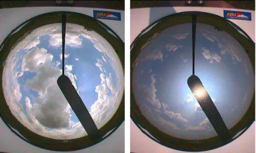
Figure 1 shows the TSI images for these two days. Visual comparison of these im-ages illustrates how aerosol may obscure clouds and clear sky from a surface observer. For the clean day (5 July), one can readily distinguish clouds against a blue sky (Fig. 1).

15

However, for the polluted day (8 July), we have a “dirty” and blurry image and clouds appear much less distinct (Fig. 1). Since aerosol is mostly non-absorbing (̟0 ∼0.95)

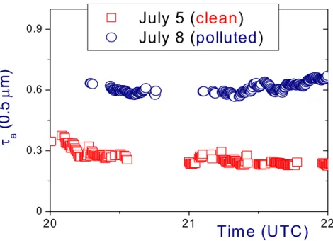
for the considered days, the observed obscuring effect is attributed mainly to the large aerosol loading (Fig. 2). In comparison with the clean day, the polluted day is char-acterized by a large aerosol burden: τa ∼0.6 at wavelength 0.5 µm, which is about

20

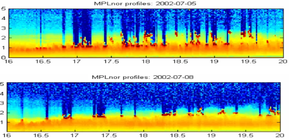
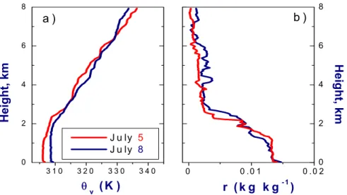
twice as large as that for the clean day (Fig. 2). From the MPL images, the selected days have no elevated aerosol layers with most aerosol located below 3 km within the boundary layer (Fig. 3). In addition, one can see that clean and polluted clouds have similar cloud base heights (∼1.5 km). Such similarity of the cloud base heights can be explained by close agreement between the thermodynamical properties (Fig. 4). Also,

25

the SMOS-derived surface winds have comparable speeds (∼4–6 m s−1) and similar preferred direction from the southeast for these days (not shown).

To ensure that the effect of cirrus contamination on the estimation of FWC

(10)

ACPD

7, 11797–11837, 2007

Full Screen / Esc

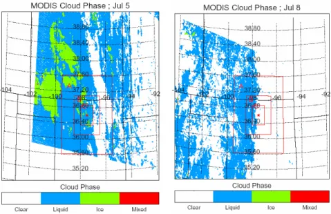
ties is not substantial, we use the MODIS observations. Figure 5 shows images of the MODIS-derived cloud phase. For the clean day (5 July), both cirrus and liquid clouds occur (Fig. 5). We estimate the fraction of cirrus clouds as the ratio of the number of pixels with cirrus clouds to the total number of cloud pixels. Cirrus fraction is esti-mated for different regions surrounding the SGP site. We use labels A, B, and C for

5

large, moderate, and small regions, respectively. The fraction of cirrus clouds is about 10% and almost region-independent. In addition to the cloud phase determination, we use the MODIS observations to examine the effective radius of droplets re. Here

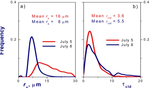
r_e is defined as the ratio of the third to second moments of the particle size distribu-tion. Figure 6 illustrates frequency distributions ofr_e obtained for region A from the

10

MODIS cloud product. Similar results are obtained for other regions (not shown). The frequency distributions ofr_e are constructed to summarize the frequency with which each r_e value occurs in the MODIS images. One can readily see that frequency dis-tributions derived for clean and polluted days are different (Fig. 6a). For large droplets (r_e>10 µm), some of these differences can be attributed to the cirrus contamination

15

of the MODIS retrievals. However, there is a substantial difference for small droplets (re<10 µm) as well (Fig. 6a). From the MODIS data, we can conclude that polluted

clouds have smaller droplets. This is consistent with previously reported results, which were obtained from observations (e.g., McFarquhar et al., 2004; Koren et al., 2005) and model simulations (e.g, Xue and Feingold, 2006; Guo et al., 2007). Since liquid

20

water path (LWP) is proportional to the product of τcld and re (e.g., Stephens, 1994)

and polluted clouds are optically thicker (Fig. 6b) and have smaller droplets (Fig. 6a), it appears that the LWP is not sensitive to the aerosol loading for the cases considered here.

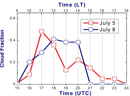
Let us consider the diurnal evolution ofN for clean and polluted clouds (Fig. 7). Here

25

theN represents the hourly averaged N obtained from the ARSCL data. The striking feature is that under polluted conditions, clouds suddenly disappear in the afternoon (after 20:00 UTC). A possible explanation might be that the ARSCL measurements have limitations. For example, the ARSCL instruments have a narrow field-of-view and

(11)

ACPD

7, 11797–11837, 2007

Full Screen / Esc

only detect clouds that occur directly above them. As a result, theN obtained from such measurements may not be representative of a larger area surrounding these instru-ments (e.g., Berg and Stull, 2002; Kassianov et al., 2005a). However, visual inspection of the TSI images confirms that the FWC clouds faded away sharply after 20:00 UTC (not shown). Compared to clean clouds, polluted clouds have much smallerN in the

5

afternoon (after 20:00 UTC) (Fig. 7). Can we observe similar difference between clean and polluted clouds from the long-term observations? The next section addresses this issue.

4 Climatology

The case study presented in the previous section suggests that clean and polluted

10

clouds may have distinct differences in terms of the diurnal variability of the cloud frac-tion (Fig. 7). To evaluate the daytime-dependence of this difference, we separate the 5-year climatology into two large groups based on time of day. These two groups repre-sent data obtained in the morning (before 20:00 UTC) and afternoon (after 20:00 UTC), respectively. For the ARCF site, local time (LT) is related to UTC as LT=UTC-6. The

15

strong diurnal cycle ofN associated with thermodynamical state variables and radia-tive properties has been frequently demonstrated (e.g., Brown et al., 2002). For the given 5-year dataset, the mean N grows in the early part of the day and reaches its maximum (∼35%) at around 20 UTC and then declines to around 15% at 24:00 UTC (Berg and Kassianov, 20071). Therefore, the data presented here are separated into

20

two groups, before and after 20:00 UTC. Such separation (i) relates to the time when the maximum mean value of N was observed (Berg and Kassianov, 20071) and (ii) represents the evolution of the FWC clouds from their initial growth (morning) to their final dissipation (afternoon).

To study the relationship betweenN and τ_a, we perform the following three-step data

25

processing procedure (analogous to Sekiguchi et al., 2003). First, we sort the hourly averaged N values into seven bins of τa (at 0.5µm) with the same increment of 0.1.

(12)

ACPD

7, 11797–11837, 2007

Full Screen / Esc

Second, we calculate the mean value ofN for each bin. Finally, these mean bin values are used to produce scatterplots ofN as function of τa. Since the frequency distribution

ofτ_ais not uniform (Fig. 8), the number of sorted N values is bin-dependent. In other words, some bins have fewerN values. For example, the first and last bins compared to others have relatively small number (∼10) of N values (Fig. 8). As a result, the

5

corresponding mean bin values ofN are less statistically robust toward both ends of the range of aerosol optical depth.

We assume that an association between N and τa can be described by a linear

regression. Figure 9 illustrates thatN is correlated with τ_a in the afternoon and the absolute value of the correlation coefficient is relatively high | r | ∼ 0.83 (Table 1a). We

10

determine the significance of the observed correlation coefficient r from the t-statistics. In particular, we use p value for the t-test of the correlation coefficient equals to 0, where smallp value indicates that the correlation between N and τ_ais significantly dif-ferent from 0. For a given correlation coefficient (| r | ∼ 0.83), the attained significance level is smallp ∼ 0.04. This means that the regression model (N versus τ_a) is usable.

15

Also, Fig. 9 shows thatN decreases with an increase of τ_a in the afternoon. This is consistent with the case study results in Sect. 3. The slope of the regression line is about –0.13 (Table 1a) and is significantly different than 0. Note, that the slope can be interpreted as the sensitivity of association. The sensitivity also can be expressed in terms of “absolute percent” (Warren et al., 2007) or changes of N in units of

per-20

centage points. We will use the “absolute percent” term in our paper. For example,N decreases from 0.31 to 0.24 in the afternoon, and thus, the change inN is 7%.

Figure 9 illustrates the strong negative correlation between N and τa in the

after-noon. The opposite is true in the morning (Fig. 9) when a relatively weak positive cor-relation (r∼0.41) is observed. The corresponding p value is relatively large (p∼0.36

25

in Table 1a) and indicates that the strength of the correlation between N and τa in

the morning is weak. Let us demonstrate that the observed positive correlation in the morning is spurious. In addition to the original regressions (Fig. 9), we constructed two alternatives by only using six points. The first point, which corresponds to the

(13)

ACPD

7, 11797–11837, 2007

Full Screen / Esc

first bin (τ_a<0.1), is excluded from consideration. As a result, the original (based on seven points) and additional (based on six points) regressions are different in terms of sign and magnitude (Tables 1a, b). However, the corresponding parameters of the afternoon regression are not sensitive to the number of points (seven versus six) (Ta-bles 1a, b). The obtained results suggest that thermodynamical and dynamical effects

5

primarily control the FWC development in the morning (early phase), while the role of aerosols on the FWC evolution increases in the afternoon (later phase).

So far, we considered the totalN, which combines contributions from both small and large clouds. How sensitive is the relationship betweenN and τ_ato the horizontal cloud size? To estimate this sensitivity, we separate the 5-year data into two additional groups

10

based on the mean horizontal cloud size. For the 5-year dataset, the mean horizontal cloud size is about 1 km (Berg and Kassianov, 20071). Data from ARSCL and the 915-MHz radar wind profiler were combined to yield the cloud chord length (CCL) (Berg and Kassianov, 20071). Since the temporal resolution of the ARSCL VAP is 10 s and the nominal error of the wind speed measured with the wind profiler is ±1 ms−1, the

15

corresponding spatial resolution of CCL (lmin) is 0.1 km. The largest value of CCL

(lmax) in our analysis is set as 6 km. A number of different factors can contribute to

large values of CCLs. For example, the distance between individual clouds and their parts/fragments can be similar to or less thanlmin, and some clouds can be tilted and

hence overlap for a nadir looking surface instrument. Similar to Rodts et al. (2003), the

20

cloud fractionN has been defined in terms of the N density (αf) as

N = lmaxZ l_min αf(l ) dl , (1) α_f(l )= 1 Ln (l ) × l , (2)

wheren is the number of clouds with a given CCL, l is the CCL, and L is the total length of interest. We have demonstrated (Berg and Kassianov, 20071) that such spatial cloud

25

(14)

ACPD

7, 11797–11837, 2007

Full Screen / Esc

fraction N is in good agreement with conventional temporal cloud fraction, which is defined as the fraction of time that a cloud is overhead (e.g., Dong et al., 2006).

For small clouds (CCL<1 km), a positive trend is observed: the cloud fraction N in-creases from 0.15 to 0.22 (∼7% change) with increasing aerosol optical depth (Fig. 10). The linear regression model does appear to be a reasonable description of the

ob-5

served relationship betweenN and τ_a (Fig. 10). In particular, the corresponding cor-relation coefficient is r∼0.67 and attained significance level is p∼0.10 (Table 1a). The parameters of the considered linear regression depend on the number of points used to compute it, but the sign of the trend is unchanged (Tables 1a, b). In contrast, the cloud fraction of large clouds shows poor correlation with τ_a (Fig. 10): the slope is

10

negative and near zero (Table 1a). The negative trend becomes more pronounced if observations with small τ_a (less than 0.1) are not considered (Tables 1a, b). These results (Fig. 10) suggest that, under polluted conditions, the relative contribution of small clouds to the totalN increases. It should be mentioned that these two groups are not independent. For example, a large cloud can be divided into smaller pieces

(frag-15

ments) during its evolution. In our analysis, these pieces of a former large cloud are considered as small clouds. The inverse process may also occur when small clouds merge into a larger one.

Since the contribution of the small clouds, which have a cloud size smaller than 1 km, to the total cloud fraction of FWC clouds is substantial (Berg and Kassianov, 20071), it

20

is difficult to infer distinct cloud-size compositions of clean and polluted clouds from the available 1-km resolution MODIS data. We will discuss this and other issues associated with the unique properties of the FWC clouds and the operational satellite retrievals in the next section.

5 Discussion

25

Our results (previous sections) provide observational support that aerosols may influ-ence the formation and evolution of low-level clouds. However, these results reveal

(15)

ACPD

7, 11797–11837, 2007

Full Screen / Esc

little about the mechanisms associated with the aerosol effects that are responsible for the changes of N. Recent large-eddy simulation (LES) studies suggested some of these mechanisms by examining the response of warm continental cumulus clouds to aerosol loading (e.g., Xue and Feingold, 2006; Jiang and Feingold, 2006). For example, Jiang and Feingold (2006) showed that aerosol radiative effects can

signif-5

icantly modify atmospheric heating profiles, reduce surface radiative fluxes, and thus decrease convection and the cloud fraction. It has also been found thatN is sensitive to microphysical-dynamical feedback (Xue and Feingold, 2006). In particular, drop-size-dependent evaporation rates may be responsible for changes in cloud size and cloud fraction (Xue and Feingold, 2006). In Sects. 5.1 and 5.2, we consider both the

10

observed radiative and microphysical effects associated with aerosol loading.

5.1 Aerosol radiative effects

As the aerosol loading increases, the aerosol blocks the surface from the incoming so-lar radiation. As a result, both the surface heating and the upward convection decrease (Jiang and Feingold, 2006). On the other hand, less intensive convection reducesN,

15

leads to less cloud shading of the ground from the sun, and thus, increases the surface insolation/heating and the upward convection. Here the surface insolation is defined as the amount of sunlight reaching the surface. Therefore, τa increasing and N

de-creasing can produce opposite changes in the surface insolation and the subsequent convection.

20

Aerosol and clouds affect both SW and LW fluxes, making it difficult to predict differ-ent and possibly compensating changes in the surface energy balance. To estimate the sensitivity of the net SW, LW, and total (SW+LW) fluxes at the surface, we separate the 5-year data into two groups. The net flux is defined as the difference between incoming and outgoing radiative fluxes. Similar to the previous analysis ofN (Sect. 4), these two

25

groups are selected based on the time of day (morning and afternoon). As expected, the net SW flux contributes most of the total flux (Table 2). In the morning, the SW and the LW fluxes have opposite trends, and thus, due to these partly compensating

(16)

ACPD

7, 11797–11837, 2007

Full Screen / Esc

changes the relationship between the total flux and τ_a is weak (Table 2). It is inter-esting that a similar weak relationship is observed betweenN and τa in the morning

(Fig. 9, Table 1a). In the afternoon, both the SW and the LW fluxes have positive trends. Such synchronized changes in the SW and LW fluxes lead to the positive and strong correlation between the total flux andτaobserved in the afternoon (Table 2). The

cor-5

responding correlation coefficient (r∼0.79) is similar to that (| r | ∼ 0.83) obtained for the cloud fraction (Table 1a). Contrary to the model results, which demonstrated the reduction of both the cloud fraction and the total flux with aerosol loading (Jiang and Feingold, 2006), the observed changes of the total flux andN have opposite signs in the afternoon (Table 1a, Table 2).

10

Aerosols can affect the surface radiation fluxes in several different ways. Let us illustrate the aerosol radiative effect by using the incoming SW flux as an example. The LW and the total fluxes can be described similarly. We start with the plane-parallel approximation and then consider a three-dimensional (3-D) case. In the context of the plane-parallel approximation, the incoming SW fluxF_pp can be written as

15

F_pp= (1 − N) Fclear+ N Fcld, (3)

whereFclearandFcldare the downward SW fluxes obtained under clear-sky and cloudy

(completely overcast) conditions, respectively.

From Eq. (3), we can estimate the sensitivity of the SW flux toτ_avariations as ∂F_pp ∂τ_a = (1 − N) ∂Fclear ∂τ_a + ∂N ∂τ_a(Fcld− Fclear)+ N ∂Fcld ∂τ_a (4a) 20

Three terms in Eq. (4a) determine the magnitude and sign of this sensitivity. Since Fclear decreases with an increase of τa, the first term is always negative. The sign

of the second term is defined completely by the partial derivative of N with respect to τa as Fcld−Fclear<0. In other words, if N decreases with τa, the second term is

positive and vice versa. The third term is a function of the cloud optical properties

25

and their sensitivity to τ_a variations. Typically, the cloud optical depthτ_cld increases 11811

(17)

ACPD

7, 11797–11837, 2007

Full Screen / Esc

with an increase of τ_a (e.g., McFarquhar et al., 2004); the opposite is true for the effective radius of cloud droplets re (e.g., Lohmann and Feichter, 2005), and thus for

the asymmetry parametergcld. These two factors (increase ofτcldand decrease ofgcld)

make the clouds more reflective (or less transparent) and thus lead to the reduction of Fcld. Therefore, the sign of the third term tends to be negative. We will discuss

5

the relationship between the MODIS-derived cloud parameters (τcld andre) andτa in

Sect. 5.2 and show that the third term appears to be positive for the FWC clouds . In a similar manner, the sensitivity of the three-dimensional (3-D) SW fluxF3D toτa

changes can be estimated as ∂F3D ∂τ_a = ∂F1 ∂τ_a + ∂F2 ∂τ_a + ∂F3 ∂τ_a (4b) 10

where the first, second, and third terms represent partial changes of F3D due to

changes in the aerosol optical characteristics, the cloud macrophysics (e.g.,N, CCL), and the cloud optical (e.g., τcld) properties, respectively. Thus, differences between

models and observations (e.g., positive versus negative trend of the total flux) can be explained partially by quantitative and qualitative differences in these terms.

15

The modeled (Jiang and Feingold, 2006) and observed (Table 1) trends of N are similar in terms of sign (negative). In contrast, the corresponding trends of the net surface fluxes obtained from model simulations and observations have slopes with op-posite signs. Thus, our findings suggest that the reduction of the surface flux resulting from an increase of τa is not the single nor most important factor for controlling the

20

N, as originally suggested (Jiang and Feingold, 2006). The modifications in the atmo-spheric heating profiles associated with the aerosol absorption may be a reason for the qualitative differences between results obtained from model simulations (Jiang and Feingold, 2006) and observations. Recall, the integrated observational dataset repre-sents mostly non-absorbing conditions (̟0∼0.95), while the model simulations (Jiang

25

and Feingold, 2006) have been performed for absorbing aerosol (̟0∼0.9), which can

be associated with biomass burning smoke. The corresponding SW radiative heating 11812

(18)

ACPD

7, 11797–11837, 2007

Full Screen / Esc

rates of the atmosphere may be as much as 6 K day−1 for this type of aerosol (Jiang and Feingold, 2006).

5.2 Aerosol microphysical effects

The importance of aerosols for altering the cloud microphysical properties is well illus-trated (e.g., Xue and Feingold, 2006; Fan et al., 2007, and bibliography therein). In turn,

5

the microphysical changes of cumulus clouds can substantially modify their amount and optical depth (Lohmann and Feichter, 2005). One reason for this modification has been suggested by Xue and Feingold (2006). An increase in aerosol concentration results in a decrease of cloud droplet size. Therefore, the polluted clouds in compar-ison with clean clouds have smaller droplets. They found that the smaller droplets of

10

polluted clouds evaporate more readily and cause a more intensive N reduction un-der the polluted environment. In other words, the droplet size response to aerosol and the drop-size-dependent evaporation rates may be responsible for distinctions between pristine and polluted cloud properties.

To estimate the sensitivity of the cloud droplets to the aerosol burdens, we perform

15

an analysis of available satellite data. In particular, we apply two MODIS datasets of cloud properties obtained from the Terra and Aqua observations. From these two datasets, we select cases that meet the following criteria. First, the satellite and sur-face observations must have occurred on the same days. Second, during the satellite observations there is a well-defined single layer of FWC clouds over both the SGP

20

site and surrounding regions. Again, we consider three different regions centered at the SGP site (Fig. 5). Similar to the case study (described in Sect. 3), we estimate the fraction of cirrus clouds for each region. If, for a given day, this fraction in a re-gion exceeds 10%, we assume that cirrus contamination is high and discard all cloud properties obtained for this day. The selected cloud properties are separated into two

25

bins. The first bin (τa<0.2) and the second bin (τa>0.2) represent clean and polluted

conditions, respectively.

(19)

ACPD

7, 11797–11837, 2007

Full Screen / Esc

Figure 11a shows the Terra-derived values of r_e for three different regions. Each region has a decrease in re with an increase in aerosol loading and the rate of this

decrease (negative trend) is region-dependent (Fig. 11a). The observed negative trend is consistent with the case study results (Fig. 6) and numerous previous stud-ies. The latter have considered mainly stratus and stratocumulus clouds and provided

5

ample evidences of the droplet size reduction by aerosol (e.g., Lohmann and Feichter, 2005). Such a reduction was originally proposed by Twomey (1977), well-known as the Twomey effect. Contrary to the stratus/stratocumulus related studies, we observe an increase inr_e with the aerosol loading for each region using the Aqua observations (Fig. 11b). Note that the Terra and Aqua observations are performed in the morning

10

(17:30 UTC) and in the afternoon (20:00 UTC), respectively. Therefore, we can spec-ulate that for the FWC clouds, the r_e−τ_a relationship is time-dependent and may be either negative (morning) or positive (afternoon). In other words, the Twomey effect is apparent only during the development of the FWC clouds and the initial stage of their evolution. Different processes are responsible for the droplet size growth/reduction

15

(e.g., Xu et al., 2005). It seems reasonable from our results that for the FWC clouds the magnitude of these processes and its sensitivity to aerosol amount depend on the time of day.

If the model-suggested direction of causality is from smaller droplets and more inten-sive evaporation to the more substantialN reduction (Xue and Feingold, 2006), then

20

there−τaand theN−τarelationships should have the same negative trends. However,

the observedr_e−τaandN−τarelationships have opposite trends in the afternoon:

neg-ative for theN−τa(Fig. 9) and positive for there−τa(Fig. 11). In other words, compared

to pristine clouds the polluted ones have larger droplets and smaller horizontal sizes. Therefore, the observations do not support the model-suggested direction of

causal-25

ity associated with smaller droplets of polluted clouds and the drop-size-dependent evaporation rates. On the other hand, the contribution of small clouds increases with the aerosol loading (Fig. 10), as the model predicts (Xue and Feingold, 2006). The observed increase of the small clouds is probably due to a combined effect of (i)

(20)

ACPD

7, 11797–11837, 2007

Full Screen / Esc

trainment rates, which are inversely proportional to the cloud size (e.g., McCarthy, 1974); (ii) the vertical profiles of heating/cooling and drying/moistening, which are very different for small and large clouds (e.g., Zhao and Austin, 2005); and (iii) the size-dependent dynamical properties of cumulus clouds (e.g., Rodts et al., 2005). As result of the combined effect, the large clouds may last longer than small clouds: the lifetime

5

for simulated small and large clouds is about 18 min and 25 min, respectively (Zhao and Austin, 2005).

Contrary to the effective radius of cloud droplets re(Fig. 11), the cloud optical depth

τcld is more sensitive to the region selection (Fig. 12). For example, the Terra-derived

τ_cldobtained for the region C is nearly twice as small as that for the region A (Fig. 12a).

10

Since τcld∼LW P/re, such stronger sensitivity is primarily attributed to region-related

variations of the LWP. The latter can compensate r_e changes associated with the aerosol loading, and as a result, can produce weak dependence between τcld and

τa. In other words, the LWP decrease (increase) may offset the re reduction (growth).

This is illustrated in the Terra-derived cloud product for regions A and B. Although the

15

effective radius redecreases with aerosol (Fig. 11a), the cloud optical depthτcldappear

to be independent ofτa(Fig. 12a). On the other hand, the effective radius re (Fig. 11b)

and cloud optical depthτcld (Fig. 12b) exhibit opposite behavior withτa for all regions

in the afternoon. This is likely due to the LWP contribution toτcld, which appears fairly

insensitive to the region selection in the afternoon.

20

The observed time-dependentN−τ_a,r_e−τ_a, andτcld−τarelationships are mainly

re-sponsible for the observed SW flux changes with aerosol (Table 2). For example, in the afternoon the polluted clouds have a smaller cloud fractionN (Fig. 9), larger droplets (Fig. 11) (or larger gcld), and smaller optical depth τcld (Fig. 12). The corresponding

observed increase of the SW flux (Table 2) can be explained as follows. The smaller

25

cloud amount reduces the cloud shading of the ground from the sun, and thus leads to more intensive surface insolation. In turn, theτcld reduction andgcld increase make

the clouds more transparent and enhance the surface insolation (warming effect) even further. Contrary to the well-known cooling aerosol effect during clear-sky conditions

(21)

ACPD

7, 11797–11837, 2007

Full Screen / Esc

(e.g., Yu et al., 2002), the warming effect of non-absorbing aerosols may be observed in a party cloudy atmosphere. It should be mentioned that the cloud shading effect is a function of the solar zenith angle (SZA),N, and cloud aspect ratio (thickness to horizontal size). At constantN and cloud aspect ratio, importance of the cloud shading increases with SZA (the sun gets lower) (e.g., Kassianov et al., 2005b).

5

Satellite remote sensing of cumulus clouds is inherently difficult as a result of their (i) low amount of liquid water (LWP,≤100 g m−2), (ii) small sizes (≤1 km), and (iii) complex 3-D geometry. Since the radiative properties of clouds with low LWP are very sensitive to the LWP changes and this sensitivity is a function of r_e, the retrieval of τ and r_e for such optically thin clouds presents a challenge even for completely overcast cases

10

with relatively weak horizontal variability (Turner et al., 2007). Moreover, the sizes of many cumulus clouds are smaller or comparable to the 1-km resolution of the typical MODIS cloud product. As a result, some pixels from a satellite image are only partially cloud covered and biases in the operational MODIS retrievals, which are based on an assumption that 1-km pixels are completely overcast, may be large. Finally, the strong

15

3-D radiative effects, associated with the complex geometry of cumulus clouds, compli-cate their remote sensing matters still further (e.g., Vant-Hull et al., 2007). Therefore, the uncertainties for cumulus retrievals are substantially larger than those for stratus or stratocumulus clouds (e.g., Kato et al., 2006). However, uncertainties for the area-averaged data considered here are much smaller than uncertainties obtained for each

20

pixel. Moreover, since the FWC clouds are observed by the same MODIS instrument launched on the Terra and Aqua platforms, the biases of the Terra and Aqua observa-tions are expected to be consistent. Therefore, the possible systematic biases of the cumulus retrievals will have no impact on observed trends.

6 Summary

25

The relationship between cloud fractionN of the fair-weather cumulus (FWC) clouds and aerosol optical depthτa is assessed using 5-year surface and Terra/Aqua

(22)

ACPD

7, 11797–11837, 2007

Full Screen / Esc

lite observations at the Atmospheric Radiation Measurement (ARM) Climate Research Facility (ACRF) Southern Great Plains (SGP) site. To reduce possible contamination of the aerosols on the estimation ofN (and vice versa), we use independent datasets ofτaandN obtained from the Multi-filter Rotating Shadowband Radiometer (MFRSR)

measurements and from the ARM Active Remotely Sensed Clouds Locations (ARSCL)

5

value-added product, respectively. Optical depth of the FWC cloudsτcld and effective

radius of cloud dropletsr_e are obtained form the MODerate resolution Imaging Spec-troradiometer (MODIS) data. The main results are as follows:

1. Both the cloud fractionN and cloud optical depth τcldexhibit a weak positive

corre-lation with aerosol optical depthτ_ain the morning, while this correlation becomes

10

significantly negative in the afternoon. It appears that the role of aerosol in the evolution of the FWC clouds increases as they mature.

2. The effective radius of cloud droplets re is negatively correlated with τa in the

morning, while the opposite is true in the afternoon. This suggests that for the FWC clouds the magnitude of droplet size growth/reduction processes and its

15

sensitivity to aerosol amount depend on the time of a day.

3. Time-dependent changes of cloud properties, associated with aerosol loading, control the day-to-day variability of surface radiative fluxes. For example, in com-parison with pristine clouds, the polluted clouds are more transparent in the after-noon due to smaller cloud fraction, smaller optical depth, and larger droplets. As

20

a result, the corresponding correlation between the surface radiative flux andτa

is positive (warming effect of aerosol).

4. Cloud fraction of large clouds (larger than 1 km) is relatively insensitive to the aerosol amount. In contrast, the cloud fraction of small clouds (smaller than 1 km) is strongly positively correlated withτa. This suggests that an ensemble of

pol-25

luted clouds has an increased number of smaller clouds than a similar ensemble in a pristine environment. The observed positive trend supports the model pre-dictions (e.g., Xue and Feingold, 2006).

(23)

ACPD

7, 11797–11837, 2007

Full Screen / Esc

5. The overall picture that emerges is that the N−τ_a relationship depends on both the time of day and the cloud size. One should be aware of these remarkable features when qualitatively comparingN−τa relationships obtained from surface

measurements, satellite observations, and model simulations. For example, the diurnal time-dependence of the N−τa relationship may lie hidden in the

daily-5

averaged statistics. The same is true for the cloud-size-averaged statistics, which combine the effect of small and large clouds.

6. The integrated dataset of aerosol, cloud, radiative, thermodynamical, and mete-orological properties obtained from the surface and satellite observations at the ACRF SGP site presented here provides a new observational constraint, which

10

can be used to ascertain performance and predictions of model simulations. Cur-rent and future parameterizations of the FWC clouds should reproduce the ob-served trends.

We stress that these conclusions are obtained for the nonprecipitating FWC clouds and the mostly non-absorbing aerosols that occur at the ACRF SGP site. Since the

SGP-15

obtained statistics appear to be fairly typical of the mid-latitude regions, we expect that the above conclusions may be valid for a range of continental FWC clouds and aerosols.

An area worthy of further research is to extend analysis of the cloud-aerosol rela-tionship by using additional observations/datasets available at the ACRF SGP site. In

20

particular, the Raman lidar (RL) measures the vertical profiles of water-vapor mixing ratio and several aerosol-related quantities (e.g., Ferrare et al., 2006), while the Atmo-spheric Emitted Radiance Interferometer (AERI) can provide cloud optical depth and effective radius of droplets with high temporal resolution (e.g., Turner, 2005). We plan to use both the RL and AERI observations to better characterize aerosol, cloud and

25

thermodynamical properties, and thus, better understand the aerosol-cloud-radiation interaction.

Acknowledgements. This work was supported by the Office of Biological and Environmental 11818

(24)

ACPD

7, 11797–11837, 2007

Full Screen / Esc

Research of the U.S. Department of Energy as part of the Atmospheric Radiation Measurement (ARM) Program. We thank M. Ovtchinnikov and D. Turner for providing useful discussions and valuable suggestions.

References

Albrecht, B. A.: Aerosol, cloud microphysics and fractional cloudiness, Science, 245, 1227–

5

1230, 1989.

Alexandrov, M. D., Lacis, A. A., Carlson, B. E., and Cairns, B.: Remote sensing of atmospheric aerosols and trace gases by means of multifilter rotating shadowband radiometer. Part I: Retrieval algorithm, J. Atmos. Sci., 59, 524–543, 2002.

Alexandrov, M., Marshak, A., Cairns, B., Lacis, A., and Carlson, B.: Automated cloud screening

10

algorithm for MFRSR data, Geophys. Res. Lett., 31, L04118, doi:10.1029/2003GL019105, 2004.

Andrews, E., Sheridan, P., Ogren, J., and Ferrare, R.: In situ aerosol profiles over the Southern Great Plains cloud and radiation test bed site: 1. Aerosol optical properties, J. Geophys. Res., 109, D06208, doi:10.1029/2003JD004025, 2004

15

Berg, L. K. and Stull, R. B.: Accuracy of point and line measures of boundary layer cloud amount, J. Appl. Meteorol., 41, 640–650, 2002.

Brown, A., Cederwall, R. T., Chlond, A., et al.: Large-eddy simulation of the diurnal cycle of shallow cumulus convection over land, Q. J. R. Meteorol. Soc., 128, 1075–1093, 2002. Clothiaux, E., Ackerman, T. P., Mace, G. G., et al.: Objective determination of cloud heights and

20

radar reflectivities using a combination of active remote sensors at the ARM CART sites, J. Appl. Meteorol., 39, 645-665, 2000.

Delene, D. and Ogren, J.: Variability of aerosol optical properties at four north American surface monitoring sites, J. Atmos. Sci., 15, 1135–1150, 2002.

Dong, X., Xi, B., and Minnis, P.: A climatology of midlatitude continental clouds from the ARM

25

SGP Central Facility. Part II: Cloud fraction and surface radiative forcing, J. Climate, 19, 1765–1783, 2006.

Fan, J., Zhang, R., Li, G., Tao, W.-K., and Li, X.: Simulation of cumulus clouds us-ing a spectral microphysics cloud-resolvus-ing model, J. Geophys. Res., 112, D04201, doi:10.1029/2006JD007688, 2007.

30

(25)

ACPD

7, 11797–11837, 2007

Full Screen / Esc

Feingold, G., Jiang, H., and Harrington, J. Y.: On smoke suppression of clouds in Amazonia, Geophys. Res. Lett., 32, L02804, doi:10.1029/2004GL021369, 2005.

Ferrare, R., Turner, D., Clayton, M., et al.: Evaluation of daytime measurements of aerosols and water vapor made by an operational Raman lidar over the Southern Great Plains, J. Geophys. Res., 111, D05S08, doi:10.1029/2005JD005836, 2006.

5

Guo, H., Penner, J., Herzog, M., and Pawlowska, H.: Examination of the aerosol indirect effect under contrasting environments during the ACE-2 experiment, Atmos. Chem. Phys., 7, 535– 548, 2007.

Hansen, J. E., Sato, M., and Ruedy, R.: Radiative forcing and climate response, J. Geophys. Res., 102, 6831–6864, 1997.

10

Harrison, L. and Michalsky, J.: Objective algorithms for the retrieval of optical depths from ground-based measurements, J. Appl. Opt., 22, 5126–5132, 1994.

Jiang, H. and Feingold, G.: Effect of aerosol on warm convective clouds: Aerosol-cloud-surface flux feedbacks in a new coupled large eddy model, J. Geophys. Res., 111, doi:10.1029/2005JD006138, 2006.

15

Jiang, H., Xue, H., Teller, A., Feingold, G., and Levin, Z.: Aerosol effects on the lifetime of shallow cumulus, Geophys. Res. Lett., 33, L14806, doi:10.1029/2006GL026024, 2006. Johnson, B. T., Shine, K. P., and Forster, P. M.: The semi-direct aerosol effect: Impact of

absorbing aerosols on marine stratocumulus, Q. J. R. Meteorol. Soc., 30, 1407–1422, 2004. Kassianov, E. I., Long, C. N., and Ovtchinnikov, M.: Cloud sky cover versus cloud fraction:

20

Whole-sky simulations and observations, J. Appl. Meteorol., 44, 86–98, 2005a.

Kassianov, E. I., Ackerman, T. P., and Kollias, P.: The role of cloud-scale resolution on radiative properties of oceanic cumulus clouds, J. Quant. Spectrosc. Radiat. Transfer., 91, 211–226, 2005b.

Kato, S., Hinkelman, L., and Cheng, A.: Estimate of satellite-derived cloud optical thickness

25

and effective radius errors and their effect on computed domain-averaged irradiances, J. Geophys. Res., 111, D17201, doi:10.1029/2005JD006668, 2006.

Kaufman, Y. and Koren, I.: Smoke and pollution aerosol effect on cloud cover, Science, 313, 3271–3274, 2006.

Kaufman, Y., Koren, I., Y., Remer, L., Rosenfeld, D., and Rudich, Y.: Effect of smoke, dust, and

30

pollution aerosol on shallow cloud development over the Atlantic Ocean, Proc. Natl. Acad. Sci., 102, 11 207–11 212, 2005.

Koren, I., Kaufman, Y. J., Rosenfeld, D., and Remer, L.: Aerosol invigoration and restructuring 11820

(26)

ACPD

7, 11797–11837, 2007

Full Screen / Esc

of Atlantic convective clouds, Geophys. Res. Lett., 32, L14828, doi:10.1029/2005GL023187, 2005.

Lohmann, U. and Feichter, J.: Global indirect aerosol effects: A review, J. Atmos. Chem. Phys., 5, 715–737, 2005.

Lohmann, U., Koren, I., and Kaufman, Y.: Disentangling the role of microphysical and dynamical

5

effects in determining cloud properties over the Atlantic, Geophys. Res. Lett., 33, L09802, doi:10.1029/2005GL024625, 2006.

McCarthy, J.: Field verification of the relationship between entrainment rate and cumulus cloud diameter, J. Atmos. Sci., 31, 1028–1039, 1974.

McFarquhar, G., Platnick, S., Di Girolamo, L., Wang, H., Wind, G., and Zhao, G.: Trade wind

cu-10

muli statistics in clean and polluted air over the Indian Ocean from in situ and remote sensing measurements, Geophys. Res. Lett., 31, L21105, doi:10.1029/2004GL020412, 2004. Michalsky, J. J., Schlemmer, J. A., Berkheiser, W. E., et al.: Multiyear measurements of aerosol

optical depth in the Atmospheric Radiation Measurement and Quantitative Links programs, J. Geophys. Res., 106, 12 099–12 107, 2001.

15

Mitchell, R., O’Brien, D., and Campbell, S.: Characteristics and radiative impact of the aerosol generated by the Canberra firestorm of January 2003, J. Geophys. Res., 111, D02204, doi:10.1029/2005JD006304, 2006.

Norris, J. R.: Has northern Indian Ocean cloud cover changed due to increasing anthropogenic aerosol?, J. Geophys. Res. Lett., 28, 3271–3274, 2001.

20

Rodts, S. M. A., Duynkerke, P. G., and Jonker, H. J. J.: Size distributions and dynamical prop-erties of shallow cumulus clouds from aircraft observations and satellite data, J. Atmos. Sci., 60, 1895–1912, 2003.

Sekiguchi, M., Nakajima, T., Suzuki, K., Kawamoto, K., Higurashi, A., Rosenfeld, D., Sano, I., and Mukai, S.: A study of the direct and indirect effects of aerosol using global satellite data

25

sets of aerosol and cloud parameters, J. Geophys. Res., 108, doi:10.1029/2002JD003359, 2003.

Sheridan, P., Delene, D., and Ogren, J.: Four years of continuous surface aerosol mea-surements from the Department of Energy’s Atmospheric Radiation Measurement Program Southern Great Plains Cloud and Radiation Testbed site, J. Geophys. Res., 106, 20 735–

30

20 747, 2001.

Stephens, G.: Remote Sensing of the Lower Atmosphere, Oxford University Press, 523 pp, 1994.

(27)

ACPD

7, 11797–11837, 2007

Full Screen / Esc

Stokes, G. M. and Schwartz, S. E.: The Atmospheric Radiation Measurement (ARM) Program: Programmatic background and design of the Cloud and Radiation Test Bed, Bull. Am. Mete-orol. Soc., 75, 1201–1221, 1994.

Turner, D. D.: Arctic mixed-phase cloud properties from AERI-lidar observations: Algorithm and results from SHEBA, J. Appl. Meteorol., 44, 427–444, 2005.

5

Turner, D. D., Vogelmann, A. M., Austin, R. T., et al.: Thin liquid water clouds: Their importance and our challenge, Bull. Am. Meteorol. Soc., 88, 177–190, 2007.

Twomey, S.: The influence of pollution on the shortwave albedo of clouds, J. Atmos. Sci., 34, 1149–1152, 1977.

Vant-Hull, B., Marshak, A., Remer, L., and Li, Z.: The effects of scattering angle and cumulus

10

cloud geometry on satellite retrievals of cloud droplet effective radius, IEEE Geo. Rem. Sens. Lett., 45, 1039–1045, 2007.

Warren, S. G., Eastman, R. M., and Haln, C. J.: A survey of changes in cloud cover and cloud types over land from surface observations, 1971–1996, J. Climate, 15, 717–738, 2007. Xu, K., Zhang, M., Eitzen, Z. A., et al.: Modeling springtime shallow frontal clouds

15

with cloud-resolving and single-column models, J. Geophys. Res., 110, D15S04, doi:10.1029/2004JD005153, 2005.

Xue, H. and Feingold, G.: Large-Eddy simulations of trade wind cumuli: Investigation of aerosol indirect effects, J. Atmos. Sci., 63, 1605–1622, 2006.

Yu, H., Liu, S., and Dickinson, R.: Radiative effects of aerosols on the evolution of the

atmo-20

spheric boundary layer, J. Geophys. Res., 107, doi:10.1029/2001JD000754, 2002.

Zhao, M. and Austin, P.: Life cycle of numerically simulated shallow cumulus clouds. Part I: Transport, J. Atmos. Sci., 62, 1269–1290, 2005.

(28)

ACPD

7, 11797–11837, 2007

Full Screen / Esc

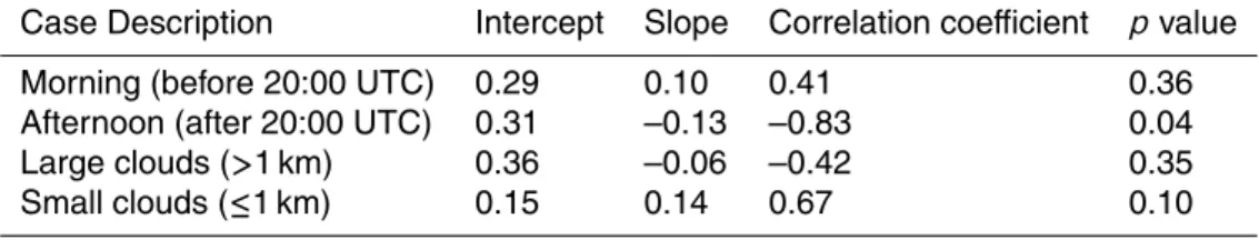
Table 1a. Fitting statistics for the linear regressions (CF versus AOD) as function of time day

(Figs. 9, 10): the intercept, slope, correlation coefficient, and p value for the t-test of the slope equals to 0. These regressions are constructed by using seven points (bins).

Case Description Intercept Slope Correlation coefficient p value

Morning (before 20:00 UTC) 0.29 0.10 0.41 0.36 Afternoon (after 20:00 UTC) 0.31 –0.13 –0.83 0.04 Large clouds (>1 km) 0.36 –0.06 –0.42 0.35 Small clouds (≤1 km) 0.15 0.14 0.67 0.10

(29)

ACPD

7, 11797–11837, 2007

Full Screen / Esc

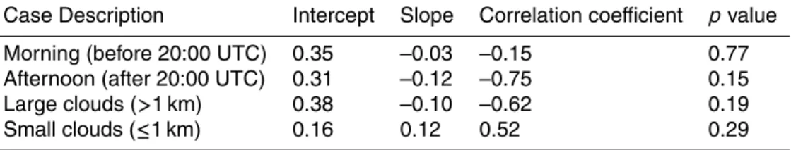
Table 1b. The same as Table 1a, except that these regressions are constructed by using six

points (bins); the first point in Figs. 9 and 10 is ignored.

Case Description Intercept Slope Correlation coefficient p value

Morning (before 20:00 UTC) 0.35 –0.03 –0.15 0.77 Afternoon (after 20:00 UTC) 0.31 –0.12 –0.75 0.15 Large clouds (>1 km) 0.38 –0.10 –0.62 0.19 Small clouds (≤1 km) 0.16 0.12 0.52 0.29

(30)

ACPD

7, 11797–11837, 2007

Full Screen / Esc

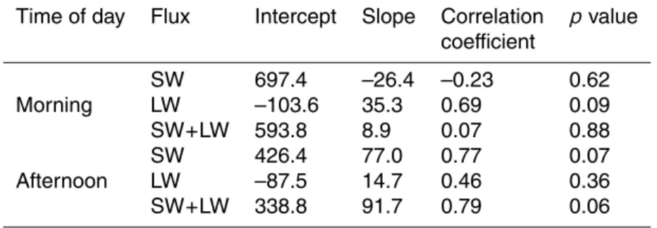
Table 2. The same as Table 1a, except that these regressions are constructed for the observed

net broadband shortwave (SW) and longwave (LW) fluxes and their sum (SW+LW). The dimen-sion of fluxes is W/m2. The fluxes are observed in the morning (16:00–20:00 UTC), and in the afternoon (20:00–24:00 UTC).

Time of day Flux Intercept Slope Correlation p value

coefficient SW 697.4 –26.4 –0.23 0.62 Morning LW –103.6 35.3 0.69 0.09 SW+LW 593.8 8.9 0.07 0.88 SW 426.4 77.0 0.77 0.07 Afternoon LW –87.5 14.7 0.46 0.36 SW+LW 338.8 91.7 0.79 0.06 11825

(31)