An evolution strategy to estimate emission source distributions on a regional scale from atmospheric observations

HAL Id: hal-00300968

https://hal.archives-ouvertes.fr/hal-00300968

HAL is a multi-disciplinary open access

archive for the deposit and dissemination of sci-entific research documents, whether they are pub-lished or not. The documents may come from teaching and research institutions in France or abroad, or from public or private research centers.

L’archive ouverte pluridisciplinaire HAL, est destinée au dépôt et à la diffusion de documents scientifiques de niveau recherche, publiés ou non, émanant des établissements d’enseignement et de recherche français ou étrangers, des laboratoires publics ou privés.

An evolution strategy to estimate emission source

distributions on a regional scale from atmospheric

observations

P. O’Brien, D. Corcoran, D. Lowry

To cite this version:

P. O’Brien, D. Corcoran, D. Lowry. An evolution strategy to estimate emission source distributions on a regional scale from atmospheric observations. Atmospheric Chemistry and Physics Discussions, European Geosciences Union, 2003, 3 (2), pp.1333-1366. �hal-00300968�

ACPD

Print Version Interactive Discussion

c

EGU 2003

Atmos. Chem. Phys. Discuss., 3, 1333–1366, 2003 www.atmos-chem-phys.org/acpd/3/1333/

c

European Geosciences Union 2003

Atmospheric Chemistry and Physics Discussions

An evolution strategy to estimate

emission source distributions on a

regional scale from atmospheric

observations

P. O’Brien1, D. Corcoran2, and D. Lowry3

1

Martin Ryan Marine Science Institute, National University of Ireland Galway, Ireland

2

Physics Department, University of Limerick, Ireland

3

Department of Geology, Royal Holloway University of London, UK

Received: 20 December 2002 – Accepted: 4 March 2003 – Published: 13 March 2003 Correspondence to: D. Corcoran (david.corcoran@ul.ie)

ACPD

Print Version Interactive Discussion

c

EGU 2003

Abstract

In this paper we present an Evolution Strategy (ES) approach towards the estimation of the location and strength of surface emissions of trace gases based on atmospheric concentration measurements and back-trajectory analyses. The details of the ES de-veloped are outlined. The ES is tested using artificial emission maps at different grid

5

resolutions and the results compared to those obtained on the same problems using Singular Value Decomposition (SVD). In almost all cases, the ES improves on SVD at equivalent resolutions. In addition, a number of insights, which the ES approach brings to the problem of source location and emission strength, are discussed, particularly the limitations on the use of measurement and meteorological data in the determination of

10

emission source distribution.

1. Introduction

In this paper, we present a novel approach towards constructing regional scale emis-sion maps from the long term monitoring of atmospheric conditions at remote sites. A common problem in atmospheric monitoring is relating measurements made at

par-15

ticular observation stations to emission sources that have influenced the sampled air mass (Seinfeld and Pandis, 1998). The motivation here is to estimate emission source strength and location using field measurements so that these independent results may be compared with emissions inventories of anthropogenic and natural sources based on economic, production and other statistical data sources. Also it is desirable to be

20

able to generate estimates for species and processes for which inventories are unavail-able.

Taking precise measurements of the concentration of important trace gases and other species in the atmosphere is both labour and capital intensive. Furthermore a limited number of suitable locations exist where the site is sufficiently remote from

25

ACPD

Print Version Interactive Discussion

c

EGU 2003

activity. Therefore, one has data which is expensive to gather, restricted to a few locations (often just a single site), from which one wishes to extract as much information as possible. In this paper, we present methods by which measurements taken at two locations can be used to estimate emissions: the remote, baseline station at the Mace Head Atmospheric Research Station, on the west coast of Ireland and a suburban field

5

site at Royal Holloway University near London (RHUL). Although the present discussion will be based on artificial measurement time series, the locations coincide with actual atmospheric monitoring stations, data from which will be incorporated into the models at a later date.

When the measurement data is combined with meteorological data, it becomes

pos-10

sible to ascribe source locations to the observed concentrations (also referred to as the excess concentrations or excess) at least qualitatively. For the Mace Head and RHUL data, contributions to the excess can come from a variety of sources particularly, but not exclusively, mainland Europe. Attempts to quantify the locations and strength of emissions sources from Mace Head, and similar data from other locations, have

how-15

ever met with varying degrees of success (Ashbaugh et al., 1985; Vasconcelos, 1996a, b; Stohl, 1996).

Recently, Ryall et al. (2001) have used a heuristic approach for determining emis-sions strengths and locations. The approach was based on the rational idea that those regions more or less often associated with higher detected gas concentrations must

20

have higher or lower emission strengths. In this paper, we present preliminary results of an alternative heuristic approach. By casting the problem as an optimisation, we investigate the use of an evolution strategy in determining the spatial distribution and strength of emissions.

2. Back trajectory analysis

25

A popular meteorological tool to investigate emission is the transport model, including the trajectory-type model (Simmonds et al., 1993; Vasconcelos, 1996a, b; Deininger

ACPD

Print Version Interactive Discussion

c

EGU 2003

and Saxena, 1997), and the dispersion-type model (Derwent et al., 1998a, b; Ryall et al., 1998, 2001; Zhang et al., 1999; Wang and Bentley, 2002). To determine emis-sion source strength and location, the model may be scaled to match observational data (Ryall et al., 2001), alternatively data assimilation techniques such as the ad-joint method (Houweling et al., 1999) or Kalman smoother (Zhang et al., 1999; Wang

5

and Bentley, 2002) can be applied. In this work, we use back-trajectory analysis and implement source characterisation using an evolution strategy.

A back trajectory is an estimate of the recent movements of an air parcel, backwards in time from the moment when the air parcel was sampled at the monitoring station. A large number of trajectory models exist, each with their own assumptions and

limita-10

tions (Kud at al., 1985; Merril at al., 1986; Draxler, 1987; Deininger and Saxena, 1997; Stohl, 1998), however all models output essentially the same type of data, which is the estimated geographical location of the air mass at preceding time intervals. Often an estimate of the height of the air parcel above the surface at the various locations visited is also part of the trajectory model output. The model results used in this paper are from

15

the Irish Meteorological Service Global Trajectory Model (GTM) using ECMWF analy-ses, details of which are given in McGrath (1989). An example of the back-trajectory data is presented in Table 1.

The injection of gas species into an air parcel depends on the parcel height and on the mixing height at the time it passed over a location. If the air parcel is above the

20

mixing height, it is assumed ground source emissions do not influence concentration. Otherwise, it is assumed that the ground emissions are mixed uniformly within the mixing height. A constant mixing height of 1000 m was used in this study and the height of the air parcel is estimated using the pressure difference between the air parcel and the surface. A consequence of these simplifying assumptions is that the solution of

25

“real-world” problems cannot be attempted. Instead the intention is to establish a “proof of concept” where a methodology for this notably complex problem is first developed and tested on artificial scenarios, but will in the future be modified to incorporate more sophisticated models of mixing height (Marik et al., 1995; Biraud et al., 2000), or actual

ACPD

Print Version Interactive Discussion

c

EGU 2003

mixing height measurements.

3. Rationale

A reasonable proposition is to combine the measurement and trajectory data in order to generate quantitative estimates of sources and their location. Following Seinfeld and Pandis (1998) the excess concentration of a species within an air mass can be

5

considered to be a result of recent influences, that is the recent emission into the air mass as it passed over source locations on its trajectory. The excess of a particular species C (as measured in ppb) arising from a trajectory j would then be the sum of emissions e (where a constant mixing height is assumed), from the geographical locations on this trajectory φ_t(a parametric curve sampled at discrete intervals of time

10

t):

C_j =X

t

e_j(φ_t). (1)

By identifying those sites, i , visited in a set of trajectories, and assuming that the emission from each location is independent of the trajectory used (also equivalent to time independence on the timescale of the trajectory set), this equation can be rewritten

15

as

C_j =X

i

n_{i , j}e_i, (2)

where n_{i , j} is a weighting factor which incorporates per trajectory the frequency with which a location has been visited and the dependence on mixing height during these visits. The weighting factor can be made as detailed as one feels necessary and can

20

include descriptions of other physical and chemical processes influencing the injection and removal of the species into the air mass. With a suitable number of observations it should be possible to solve the resulting set of simultaneous equations for e_i using

ACPD

Print Version Interactive Discussion

c

EGU 2003

standard approaches to matrix inversion (see e.g. Veltkamp at al., 1995). Unfortu-nately, the resultant matrix is sparse, can be under or over-determined, depending on the resolution of the location sampling, and, susceptible to error and model assump-tions.

4. Evolution strategy-cost function

5

An evolution strategy (ES) is an artificially intelligent global optimisation technique based loosely on the theory of evolution, i.e. survival of the fittest. The general op-eration of this technique is as follows. The vector Xopt= (x1...xn) at which the function

f (X ) is a minimum/maximum is to be determined. In general f (X ) is referred to as a

cost function if the objective is minimisation and a fitness function if maximisation (here

10

minimisation will be considered). For a vector space of many dimensions with a com-plicated surface geometry, the problem will be intractable analytically. The approach of an ES is to create a population of random solution vectors Xj referred to in ES ter-minology as chromosomes. The elements of the vectors are referred to as genes in keeping with the genetic analogy. The process of solving for Xoptinvolves continually

15

establishing the cost of each chromosome and iteratively breeding new populations until the cost function is a minimum. Usually the breeding of new populations involves the operations of selection followed by recombination/crossover and mutation. The ES is closely related to the Genetic Algorithm (Mitchell, 1996) and the distinction between these approaches is often blurred.

20

In the methodology of an ES a trial solution is attempted, the so-called chromosome from above, and rated according to how close it is to the desired solution. Its sur-vival into successive iterations of populations and its influence on the optimum solution depends on this rating. The method of rating requires a cost function which is now considered.

25

coor-ACPD

Print Version Interactive Discussion

c

EGU 2003

dinates x, y (see Fig. 1). We rewrite Eq. (2) in terms of the indices x, y,

C_j =X

x

X

y

n_{x, y, j}e_{x, y}. (3)

Sites not visited are also included in this formulation, but for these n_{x, y, j} = 0 and they are not included in the calculations (see also below). The objective is then given a set of observations C_j and associated back-trajectory data from which n_{x, y, j} can be

5

calculated, to determine the map e_{x, y} which satisfies Eq. (3). This condition can be rewritten in terms of the function f_j

f_j(e_{x, y})= C_j−X

x

X

y

n_{x, y, j}e_{x, y} = 0 (4)

and the problem becomes one of optimisation by requiring a value of e_{x, y} which min-imises the cost function.

10

F (e_{x, y})=X

j

|f_j(e_{x, y})| (5)

5. Evolution strategy-algorithm

We now describe in detail the operation of the ES which minimises the cost function of Eq. (5). The first step involved is the formation of the initial population of trial solutions

e_{x, y}. This population is generated with as few a priori assumptions as possible. In

15

general for inverse emission modelling methods, it is necessary to supply a priori infor-mation about the source activity, and perhaps more importantly the uncertainty of the emission strength. The a priori source locations are typically derived from inventories compiled from economic statistics and other literature sources. Whilst these methods progress to constrain and modify the initial information, the methodology here will

al-20

ACPD

Print Version Interactive Discussion

c

EGU 2003

the literature, for example, emissions from activities that are neither socially nor eco-nomically important. The ES will eventually provide a means of estimating emissions from regions, e.g. the north Atlantic; for species, e.g. DMS; and for processes, e.g. methane seepage from ocean floor methane hydrate deposits, for which inventory are not currently available, or are far from reliable. Application of the ES, in the future, to

5

such species as methane will provide a competitive testing ground for this method of source location and quantification against the positive results of the myriad of other approaches.

To formulate the trial solutions, use is made of two conditions. Firstly, it is impractical to assign an emission strength to a cell (where a cell is an individual element of the

10

matrix e_{x, y}) which has not been visited by the set of back trajectories i.e. those for which n_{x, y, j} = 0. Secondly, the maximum emission possible from a given cell, denoted

eT_{x, y}, is never expected to exceed the minimum concentration detected at the sampling site for any of back trajectories which have passed over the cell. In general this is probably a generous over estimate of the possible emission from a given cell. This

15

condition also places a heavy weighting on the validity of the individual trajectory with the minimum concentration. Other schemes for limiting the first guess emission from a cell can be devised, for example using the mean observed concentration associated with the given cell rather than the minimum.

Subject to these conditions the trial solution consists of a random number of visited

20

cells. A random emission strength is assigned to each cell which is less than or equal to the minimum site concentration associated with any trajectory that has passed over that cell. In total a population of typically 40 trial solutions or chromosomes is generated.

The ES then progresses as follows. The population is rated according to the cost function of Eq. (5). Subsequently the lower performing 20% of the population are

25

replaced. The methodology of replacing these solutions is now described. Firstly selection occurs. Two solutions X and Y are chosen from the surviving population, i.e. the top 80%, and combined to produce two “offspring” x and y. X is chosen at random from the top 20% of the population while Y is chosen from the entire surviving

ACPD

Print Version Interactive Discussion

c

EGU 2003

population. Those solutions of the lowest 20% are thus prevented from being involved in the replacement process.

Subsequently reproduction takes place. A weighted random binary mask typically 75% in favour of the chromosome X is generated which is used to perform a non-uniform crossover between the genes or elements of X and Y to form x and y. In this,

5

75% of the gene material of x comes from X, the remainder from Y and vice versa for y. The gene information is so far unchanged. Mutated offspring are also generated. To do this a random number of genes in both x and y are replaced (typically 10%) to produce xm and ym. For those cells selected to be mutated, the algorithm employed is the following 10 em_{x, y} = rand(0 → ±1) ∗ e T x, y M ! + ex, y em_{x, y} =      em_{x, y} 0 < em_{x, y} ≤ eT_{x, y} eT_{x, y} em_{x, y} > eT_{x, y} rand(0→1)∗eT_{x, y} M e m x, y ≤ 0 (6)

with M = qN_gen for what is termed restrained mutation and M = 1 for unrestrained mutation. Here N_gen is the number of new populations which have been generated since the ES commenced. For restrained mutation the mutation rate decreases as the

15

ES progresses.

Subsequent to mutation, the cost of all new chromosomes are evaluated and a new member of the population is taken from either x or xm depending on which has the lowest cost. The same is true of y and ym. The process of selection and reproduction is then repeated until the lower 20% of the population is replaced. The population

20

is once again ordered according to minimum cost and the entire process repeated until a maximum number of iterations/generations (taken here to mean one complete processing of the population) is exceeded or the cost-value of the function falls below a desired tolerance, and an optimum solution is determined.

ACPD

Print Version Interactive Discussion

c

EGU 2003

It is a matter of personal judgement what proportion of the population is discarded per generation. If a large proportion of the population is discarded, there may be lim-ited diversity in the remaining population. In effect the gene pool is reduced sharply. A stable population of similar solutions is thus attained in a relatively small number of generations before convergence on an optimum solution is obtained. Discarding a low

5

proportion of the population, in contrast, guarantees greater diversity in the population, at least in the earlier generations, allowing poorer solutions to progress into later gener-ations, and allowing the possibility of their gene material to contribute to later offspring. As a result it may take a greater number of generations to tend towards an optimum solution, but that solution may be of lower cost.

10

6. Case studies

To investigate the ES approach for the estimation of emission source distributions a “re-verse engineering” strategy was adopted (Doyle et al., 1999). Artificial emission maps were generated, then using a catalogue of back-trajectory analyses from 1996 to 2000 (McGrath, 1989) for Mace Head and RHUL (Lowry et al., 2001), an artificial time series

15

of concentration measurements at the sample sites was constructed. In principle given the artificial series and the associated back-trajectory data, the ES approach should be able to re-generate the corresponding emission map. For comparison, Singular Value Decomposition (SVD) was also applied to this synthetic data. SVD (Press et al., 1994) is a well understood method of solving simultaneous equations which ignores

incon-20

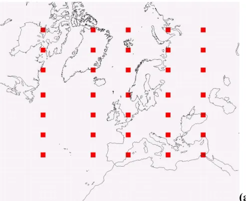
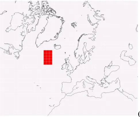
clusive or ambiguous data in favour of generating a more robust and realistic solution. Three test geometries were considered (see Fig. 2). For the area and distributed source test geometries the grid cell size is 200 × 200 km2, for the enclosing source the grid cell size is 100 × 100 km2, and in all cases the emission rate per source cell is 100 ppb/hr (recall a constant mixing height of 1000 m is assumed). The distributed

25

source problem consists of a 7 × 5 array of isolated sources with a horizontal spacing of 1000 km for column elements 2 to 5, a spacing of 1800 km for column elements 1

ACPD

Print Version Interactive Discussion

c

EGU 2003

to 2 and a vertical spacing of 600 km. The area source problem consists of a 5 × 3 array of sources located to the northwest of Ireland. Finally the enclosing source has a hexagonal outline consisting of 60 connected sources.

The ES and SVD were applied to the distributed and area geometries at 3 grid reso-lutions, with cell sizes of 100 × 100 km2, 200 × 200 km2, and 400 × 400 km2. In Fig. 3,

5

the number of visitations by the back-trajectories per cell is shown. As the resolution of the grid increases, on average the number of visitations per cell decreases. The benefit of improved resolution might therefore be expected to be at the cost of less information per cell upon which to base any estimation of emission.

The general parameters used for the ES and SVD are outlined in Table 2. As

men-10

tioned earlier two methods of mutation are available and to test this, adopting a grid size comparable to the test problem resolution, both methods were implemented on the area source problem. The convergence data for this test is shown in Fig. 4 which clearly demonstrates the significantly faster convergence character of unrestrained mu-tation. Notice also the characteristic exponential like convergence of the ES approach

15

a recognised advantage of such techniques. Given the improved performance, unre-strained mutation was adopted for subsequent ES applications.

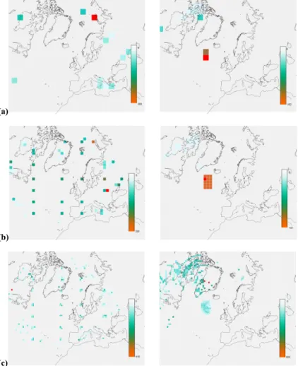
In Figs. 5 and 6 results of the ES (after 300 iterations) and SVD methods are shown for the distributed and area test geometries at each of the differing resolutions. Inspec-tion of the data clearly demonstrates that in almost all cases the ES improves over the

20

SVD results when compared at equivalent resolutions.

For both the artificial area and distributed source problems, the best ES solutions are for the grid with element size 200 × 200 km2, the resolution at which the test prob-lems were generated. In the case of the area solution a mean area emission rate of 99.9 ppb/hr (σ= 1.2) is obtained.

25

The ES does not generate an adequate solution for the distributed point source array problem at the lowest resolution and misses the sources entirely. The cause of this effect is the initialisation scheme. During the initialisation of the ES, the maximum emission value for a given cell is constrained to never exceed the minimum observed

ACPD

Print Version Interactive Discussion

c

EGU 2003

concentration associated with any trajectory which has passed through the cell. The validity of this approach however depends on the grid resolution. As seen from the visitation map (Fig. 3) as the grid cell size becomes larger an increasing number of trajectories will pass through a given cell on average. Consider now a source in a cell with physical size smaller than the grid resolution. The larger the trajectory number that

5

pass through the cell the greater the likelihood that one or more of these trajectories will not intersect the source within it. The cell strength may then be constrained by emissions from a trajectory external to the source, which is incorrect. The minimisation constraint will only be valid provided the grid cell size is smaller than the source size. The same effect is responsible for the diminished extent of the area distribution solution

10

at low resolution. It is worth pointing out that this constraint can be relaxed or even removed and an improved solution likely obtained. The trade- off would be an increase in the number of iterations required for convergence.

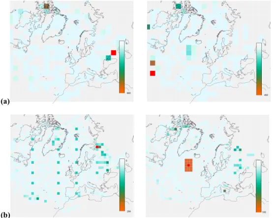
For the distributed source array at the lowest resolution (400 × 400 km2) SVD does not present a realistic solution, but at medium resolution the sources are visible. The

15

area emission source is only clearly identifiable at a medium resolution where the mean area source emission rate is 99.3 ppb/hr (σ = 0.9) compared with the correct solution of 100 ppb/hr. Importantly, in all SVD solutions there is large area coverage of spurious emission which is both positive and unphysically negative. Without prior knowledge of the distribution it would be impossible to distinguish the true distribution of sources

20

from artefact sources.

At the highest resolution 100×100 km2for both the distributed and area source prob-lems the correct solution is matched by the ES, though a variation in source solution emission is evident. The variation is most likely caused by the increasing number of unknowns at higher resolution and the limit imposed on the maximum number of ES

25

iterations. In Fig. 7 the convergence trend for the high resolution distributed source is presented, and reveals continuing convergence beyond the 300 iteration limit. In stark contrast SVD fails completely at this resolution and provides no result. Even though the information available to the ES approach is limited, a strength of the technique is that

ACPD

Print Version Interactive Discussion

c

EGU 2003

it manages to use this information efficiently to determine a solution approximation. Scattergram plots at the benchmark 300 iterations for the ES solutions of the area source problem are presented in Fig. 8. The plots display the correlation between site concentrations for each back trajectory, calculated from the optimum solutions, versus the actual site concentrations generated from the corresponding artificial maps. For

5

an exact solution a regression coefficient of unity would be obtained. From the plots it is possible to see the trend, already apparent in the solution maps above, is repeated with the best solutions obtained for the medium and high resolution grids.

One potential difficulty with the ES is the presence, particularly to the northwest, of false sources being located at the extremities of the map (see Fig. 5). This behaviour

10

is a recurring feature, though not exclusively, of the ES technique. In Fig. 6, in addition to a background of spurious emission, similar false sources can be identified for the SVD solutions, particularly to the east. In both cases, without prior knowledge of the distribution, it could be impossible to distinguish the true sources from artefact sources. In contrast to SVD however, the spurious emission appears to be confined in the ES

15

solutions only to specific areas and might therefore be identified by other means. For example comparison of the cell visitation map with the solution map shows clearly that the artefacts are located within a region of low trajectory visitation.

It is easy to understand why errors at the extremes of the ES solutions happen; the ES does not know when an injection occurs and therefore can assign emissions to all

20

locations along a trajectory if it wishes. If a cell is visited by only one or relatively few air masses, the cost function which is cumulative, is less sensitive to these cells than it is to cells which are visited on many occasions. Therefore, it is efficient for the ES to assign the relatively large emission to a single, poorly sampled cell. Under the present formulation of the ES, there is no forcing or weighting factor which informs the ES that

25

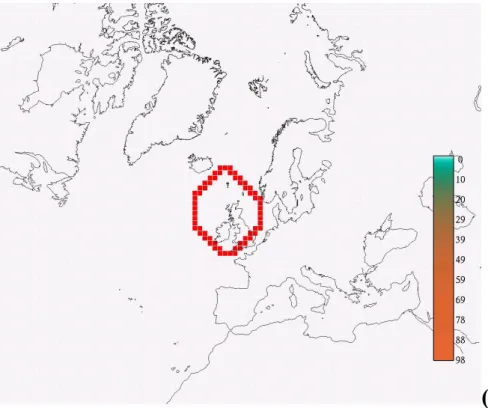
it is “wrong” to do so. Without greater a priori input, the ES cannot learn of the mistake. In Fig. 9 the results obtained from the ES at a resolution of 100 × 100 km2, for the enclosing source geometry, is shown. The ES has only limited success, with this ge-ometry. Although the inner limits of the source region is clearly defined, outside the

ACPD

Print Version Interactive Discussion

c

EGU 2003

circle is very poorly reconstructed. It would appear that in order for the ES to clearly delineate a source, a “clean” pathway to the sampling site must exist nearby. The ES needs to be able to contrast heavily burdened air masses with “clean” air masses with a similar trajectory in order to enclose the source. The SVD failed to converge on a solution for this test.

5

Overall for the ES if the emission sources fully encompass the detection sites, or when there is a lack of trajectory coverage, the ES has greater difficulty in reconstruct-ing the “true” distribution. Greatest success is had with localised sources, within well sampled regions. It can be argued therefore that high emission source regions identi-fied by the ES which are enclosed within well sampled lower/zero emission regions on

10

a reconstructed map are likely to be reliable indicators of actual source locations and emission strength. In contrast those cells at the extremes of trajectories, or part of a contiguous link to the extremes of the sampled region, are not conclusive indicators of the presence of source activity within the cells involved. Note that the argument often made, that the tendency of back trajectory studies to locate sources at the limits of their

15

range indicates the real sources lie further afield, is not valid in the test case studies.

7. Conclusions

In this paper, a novel approach has been presented to estimate the distribution of emission sources on a regional scale based on the use of evolutionary optimisation and back-trajectory analysis. An ES, that is an artificially intelligent global optimiser,

20

was developed for this purpose.

The results of the ES have been compared to the Singular Value Decomposition ma-trix method of solving systems of linear equations. The methods have been applied to the geometric test problems of an area source, a distributed source and an enclosing source, where constant emission for the test source elements was chosen. To

gen-25

erate both the test problems and solutions, a constant mixing height was assumed for the back-trajectory analyses. The use of artificial test problems also excludes both

ACPD

Print Version Interactive Discussion

c

EGU 2003

model and measurement errors which would be present in a real world scenario. Given these limitations, comparison of the ES to SVD is favourable at equivalent resolutions, with the ES approach being more successful in both the location and quantification of source emissions. At high resolution the SVD method fails to converge on any viable solution.

5

For the operation of the ES no a priori emission data was assumed. The gener-alised approach allows, in principle, for the determination of emission locations and strengths in cases where inventories are either unavailable or possibly incorrect. Nev-ertheless, if reliable inventories are available this data could be used to initialise the ES solutions. For example, a potential difficulty with the ES and also, for that matter

10

SVD, is a tendency to locate false emissions at the extremes of the trajectories. For the ES, the cost function formulated above is insensitive to the emission values asso-ciated with infrequently visited cells. With certain species it may be possible to exclude falsely identified regions by virtue of a priori knowledge of the nature of the emission sources, and so further refine the cost function. As a specific example, HCFC’s are

15

strictly anthropogenic, and significant sources must be land based. Therefore, one might exclude ocean regions from the ES from the beginning. Nevertheless, it is more often not possible to predetermine possible source regions in this manner.

Comparing the operation of the ES at different resolutions has revealed that, as might be intuitively expected, the best solution is obtained at the resolution of the

orig-20

inal test problem. In a real-world application the size of sources to be identified may not be known in advance. It has been shown, however, that at higher resolution, the test sources are located, though at computational expense. Ultimately higher grid res-olutions will be limited by low trajectory number per cell, which has been identified as a likely cause of spurious source emission. At low resolution, it is expected that

remov-25

ing the minimisation constraint, imposed on the initialisation of threshold emissions, will lead to successful source identification, though its removal will also be computationally expensive. Thus regardless of resolution, it is expected that the ES will converge on a solution provided that the trajectory visitation per cell is sufficiently high. In this

con-ACPD

Print Version Interactive Discussion

c

EGU 2003

text, it would be worth exploring an adaptive grid approach, where the grid element size distribution might be adjusted to generate an optimum trajectory visitation number per cell.

The most exacting test piece investigated was the enclosing source, for which the ES established the inside boundary only. Such a test may be representative of any

5

sampling site where the arriving air mass always passes over an emission source, as might be the case for a continental site, for example. SVD failed definitively for this test, and without the contrast of a proper background or clean concentration level, it is likely that any inverse modelling approach would have difficulty with source charac-terisation. Nevertheless, the use of a more sophisticated physical model, such as a

10

dispersion instead of a trajectory model, might lead to better characterisation, given its more refined description of potential areas which have an influence on the sampled air mass. It should be pointed out that the use of an ES approach need not be confined to back-trajectory analyses. The problem need only be cast in terms of a cost function where the model relating emissions to observation can be as complex as required.

15

Regardless of the model adopted, consideration will need to be given in the future to measurement and modelling errors for the solutions to real measurement data.

Finally, it is recognised that the presence of spurious sources undermines the results obtained from the ES approach. This could be an indication that the information which we seek may not be discernible from the data. Certainly the appearance of localised

20

false sources in the SVD solutions would support this reasoning. The ES and indeed other methods may yield results which reconstruct observed time series of measure-ments for example, but there is no guarantee that the emissions maps constructed represent reality. The constructed map is just one which is a solution to the mathemati-cal problem posed. In this debate the authors are of the opinion that the ES represents

25

an interesting new approach to the problem, which although may not (as yet) yield an exact solution, presents important insight into the complexity of problems often hidden in the more analytical approaches.

provi-ACPD

Print Version Interactive Discussion

c

EGU 2003 sions of back trajectory data to the Atmospheric Physics Group at National University of Ireland,

Galway.

References

Ashbaugh, L. L., Malm, W. C., and Sadeh, W. Z.: A residence time probability analysis of sulfur concentrations at Grand Canyon National park, Atmos. Environ., 19, 1263–1270, 1985.

5

Biraud, S., Ciais, P., Ramonet, M., Simmonds, P., Kazan, V., Monfray, P., and O’Doherty, S.: Eu-ropean greenhouse gas emissions estimated from continuous atmospheric measurements and radon 222 at Mace Head, Ireland, J. Geophys. Res., 105, 1351–1366, 2000.

Deininger, C. K. and Saxena, V. K.: A Validation of back trajectories of air masses by princi-pal component analysis of ion concentration in cloud water, Atmos. Environ., 31, 295–300,

10

1997.

Derwent, R. G., Simmonds, P. G., Doherty, S., and Ryall, D. B.: The Impact of the Montreal Protocol on Halocarbon concentrations in Northern Hemisphere Baseline and European Air Masses at Mace Head, Ireland over a ten year period from 1987–1996, Atmos. Environ., 32, 3689–3702, 1998a.

15

Derwent, R. G., Simmonds, P. G., Doherty, S., Ciais, P., and Ryall, D. B.: European source strengths and Northern Baseline Concentrations of Radiatively Active Trace Gases at Mace Head, Ireland, Atmos. Environ., 32, 3703–3715, 1998b.

Doyle, S., Corcoran, D., and Connell, J.: Automated mirror design using an evolution strategy, Optical Engineering 38, 323–333, 1999.

20

Draxler, R. R.: Sensitivity of a Trajectory Model to the Spatial and Temporal Resolution of the Meteorological Data during CAPTEX, J. of Climate & Applied Meteorology, 26, 1577–1588, 1987.

Houweling, S., Kaminski, T., Dentener, F., Lelieveld, J., and Heimann, M.: Inverse modelling of methane sources and sinks using the adjoint of a global transport model, J. Geophys. Res.,

25

104, 26137–26160, 1999.

Kud, Y. H., Skumanich, M., Haagenson, P. L., and Chang, J. S.: The Accuracy of Trajectory Models as Revealed by the Observing System Simulation Experiments, Monthly Weather Review, 113, 1852–1876, 1985.

Lowry, D., Holmes, C. W., Rata, N. D., O’Brien, P., and Nisbet, E. G.: London methane

ACPD

Print Version Interactive Discussion

c

EGU 2003

sions: Use of diurnal changes in concentration and d13C to identify urban sources and verify

inventories, J. Geophys. Res. Atmos., 106, 7427–7448, 2001.

Marik, F. J., Fischer, K. W., McDonald T. D., and Samson, P. J.: Comparison of Methods for Estimating Mixing Height Used during the 1992 Atlanta Field Intensive, J. of Applied Meteo-rology, 34, 1802–1814, 1995.

5

McGrath, R.: Global Trajectory Model, Internal Memorandum Met Eireann, 1989.

Merril, J. T., Bleck, R., and Boudra, D.: Techniques of Lagrangian Trajectory Analysis in Isen-tropic Coordinates, Monthly Weather Review, 114, 571–581, 1986.

Mitchell, M.: An introduction to Genetic Algorithms, MIT Press, Cambridge Massachusetts, 1996.

10

Press, W. H., Teukolsky, S. A., Vettering, W. T., and Flannery, B. P.: Numerical Recipes in C, Cambridge University Press, New York, 1994.

Ryall, D. B., Maryon, R. H., Derwent, R. G., and Simmonds, P. G.: Modelling long range trans-port of CFCs to Mace Head, Ireland, Quarterly Journal of the Royal Meteorological Society, 124, 417–446, 1998.

15

Ryall, D. B., Derwent, R. G., Manning, A. J., Simmonds, P. G., and O’Doherty, S.: Estimating source regions of European emissions of trace gases from observations at Mace Head, Atmos. Environ., 35, 2507–2523, 2001.

Seinfeld, J. H. and Pandis, S. N.: Atmospheric Chemistry and Physics, Wily Interscience, New York, 1998.

20

Simmonds, P. G., Cunnold, D. M., Dollard, G. J., Davies, T. J., McCulloch, A., and Derwent, R. G.: Evidence of the phase out of CFC use in Europe over the period 1987–1990, Atmos. Environ., 27, 1397–1407, 1993.

Stohl, A.: Trajectory statistics – A new method to establish source-receptor relationships of air pollutants and its application to the transport of particulate sulfate in Europe, Atmos. Environ.,

25

30, 579–587, 1996.

Stohl, A.: Computation, accuracy and applications of trajectories – A review and bibliography, Atmos. Environ., 32, 6, 947–966, 1998.

Vasconcelos, L. A. de P.: A tracer calibration of back trajectory analysis at the Grand Canyon, J. Geophys. Res., 101, 19329–19336, 1996a.

30

Vasconcelos, L.A. de P.: Spatial resolution of a transport technique, J. Geophys. Res., 101, 19337–19342, 1996b.

ACPD

Print Version Interactive Discussion

c

EGU 2003 Beemsterboer, B., Zwaagstra, O., Mols, J. J., Hensen, A., and Wyers, G. P.: Validation of

Methane Source Strengths. The Netherlands Energy Research Foundation (ECN) Report ECN-C95-034, 1995.

Wang, Y.-P. and Bentley, S. T.: Development of a spatially explicit inventory of methane emis-sions from Australia and its verification using atmospheric concentration data, Atmos.

Envi-5

ron., 36, 4965–4975, 2002.

Zhang, X. F., Heemink, A. W., Janssen, L. H. J. M., Janssen, P. H. M., and Sauter, F. J.: A

computationally efficient Kalman smoother for the evaluation of the CH₄ budget in Europe,

Applied Mathematical Modelling, 23, 109–129, 1999.

ACPD

Print Version Interactive Discussion

c

EGU 2003

Table 1. Sample back trajectory data

Trajectory number 1

Start: Lat 53.3◦N Pressure level 1000 hpa

Time 12:00 UTC on 12.12.0

Lon 0.0◦W

End: Time 12:00 UTC on 8.12.0

Forecast fields from Time 18:00 UTC on 12.12.0

Hours Lat Lon Level U-wind V-wind W-wind Ps

0 53.3◦N 9.9◦W 1000 −1.1 −5.3 −0.06 981 1 53.47◦N 9.84◦W 980.4 −5.5 0.9 −0.08 981.9 2 53.44◦N 9.6◦W 981.1 −3.5 1.7 −0.07 982.5 3 53.38◦N 9.46◦W 981.9 −1.8 2.4 −0.06 983.4 4 53.3◦N 9.4◦W 983 −0.2 3 −0.06 984.7 5 53.2◦N 9.43◦W 985 1.3 3.2 −0.05 986.4 6 53.09◦N 9.54◦W 986.8 2.9 3.6 −0.05 988.5 7 52.96◦N 9.7◦W 988.7 3.1 4.5 −0.06 989.8 8 52.8◦N 9.87◦W 989.6 3.9 6.1 −0.08 991.4 9 52.59◦N 10.09◦W 992.4 4.5 6.9 −0.08 993.5 10 52.35◦N 10.35◦W 993.6 5.9 8.7 −0.09 995.7 11 52.07◦N 10.68◦W 996.6 6.7 9.1 −0.08 997.7

ACPD

Print Version Interactive Discussion

c

EGU 2003

Table 2. Parameters used for the ES and SVD

Analysis Population Generations Mutation Crossover Replacement X/Y

ES Enclosing

source 100 300 Unrestrained 0.25 0.2 0.2/0.8

Area Source,

long run 100 1000 Unrestrained 0.25 0.2 0.2/0.8

All other

analyses 40 300 Unrestrained 0.25 0.2 0.2/0.8

SVD W_minthreshold (Press et al., 1994)

ACPD

Print Version Interactive Discussion

c

EGU 2003

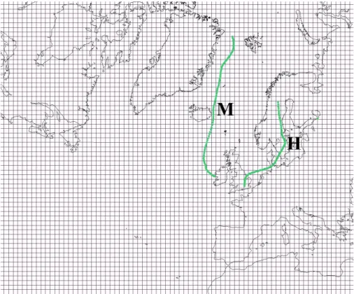
Fig. 1. The map and an example of the superimposed rectilinear coordinate graticule

with cell size 100x100 km2 used in subsequent simulations. Sample back-trajectories arriving at Mace Head (M) and Royal Holloway, University of London (H) are shown.

Fig. 1. The map and an example of the superimposed rectilinear coordinate graticule with cell

size 100 × 100 km2used in subsequent simulations. Sample back-trajectories arriving at Mace

Head (M) and Royal Holloway, University of London (H) are shown.

ACPD

Print Version Interactive Discussion c EGU 2003

(a)

(b)

(c)

Fig. 2. Test geometries for the artificial emission maps: (a) distributed source (b)

area source and (c) enclosing source.

Fig. 2. Test geometries for the artificial emission maps: (a) distributed source (b) area source

and(c) enclosing source.

ACPD

Print Version Interactive Discussion c EGU 2003

(a)

(b)

(c)

Fig. 2. Test geometries for the artificial emission maps: (a) distributed source (b)

area source and (c) enclosing source.

Fig. 2. Continued.

ACPD

Print Version Interactive Discussion c EGU 2003

(a)

(b)

(c)

Fig. 2. Test geometries for the artificial emission maps: (a) distributed source (b)

area source and (c) enclosing source.

ACPD

Print Version Interactive Discussion c EGU 2003

(a)

(b)

(c)

Fig. 3. A map revealing the number of cell visitations by back-trajectories at the (a)

low 400x400 km

, (b) medium 200x200 km

and (c) high 100x100 km

resolutions.

Fig. 3. A map revealing the number of cell visitations by back-trajectories at the (a) low 400 ×

400 km2,(b) medium 200 × 200 km2and(c) high 100 × 100 km2resolutions.

ACPD

Print Version Interactive Discussion c EGU 2003

(a)

(b)

(c)

Fig. 3. A map revealing the number of cell visitations by back-trajectories at the (a)

low 400x400 km

, (b) medium 200x200 km

and (c) high 100x100 km

resolutions.

Fig. 3. Continued.

ACPD

Print Version Interactive Discussion c EGU 2003

(a)

(b)

(c)

Fig. 3. A map revealing the number of cell visitations by back-trajectories at the (a)

low 400x400 km

, (b) medium 200x200 km

and (c) high 100x100 km

resolutions.

ACPD

Print Version Interactive Discussion

c

EGU 2003

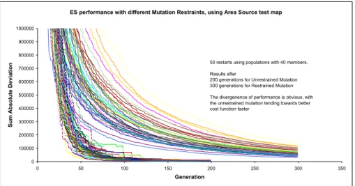
Fig. 4 The convergence trends of the ES for various start conditions for restrained

and unrestrained mutation applied to the area source problem for a 200x200 km2 cell

size.

ES performance with different Mutation Restraints, using Area Source test map

0 100000 200000 300000 400000 500000 600000 700000 800000 900000 1000000 0 50 100 150 200 250 300 350 Generation S u m A b solute D eviation

50 restarts using populations with 40 members. Results after

200 generations for Unrestrained Mutation 300 generations for Restrained Mutation The divergenence of performance is obvious, with the unrestrained mutation tending towards better cost function faster

Fig. 4. The convergence trends of the ES for various start conditions for restrained and

unre-strained mutation applied to the area source problem for a 200 × 200 km2cell size.

ACPD

Print Version Interactive Discussion c EGU 2003 (a) (b) (c)

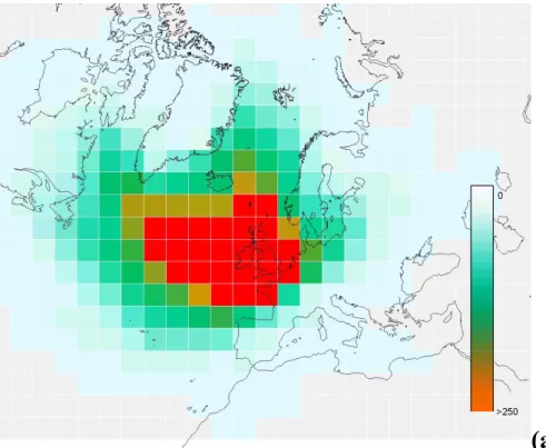
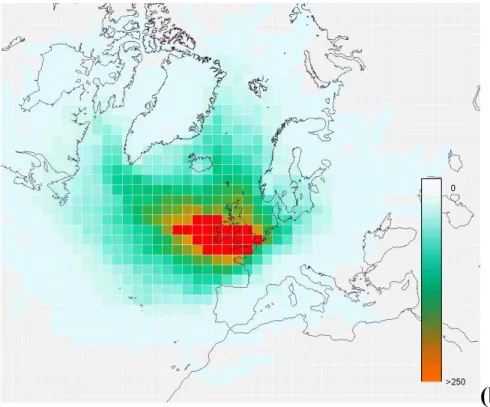
Fig. 5 Solution emission maps generated by ES for the distributed source (left) and

area source (right) at (a) low, (b) medium and (c) high resolutions.

Fig. 5. Solution emission maps generated by ES for the distributed source (left) and area

source (right) at(a) low, (b) medium and (c) high resolutions.

ACPD

Print Version Interactive Discussion c EGU 2003 (a) (b)

Fig. 6 Solution emission maps generated by SVD for the distributed source (left) and area source (right) problems at (a) low and (b) medium resolutions.

Fig. 6. Solution emission maps generated by SVD for the distributed source (left) and area

source (right) problems at(a) low and (b) medium resolutions.

ACPD

Print Version Interactive Discussion

c

EGU 2003

Progress of ES towards minimum Cost Function for Distributed Source

0 2E+10 4E+10 6E+10 8E+10 1E+11 1.2E+11 1.4E+11 1.6E+11 1.8E+11 0 200 400 600 800 1000 1200 Iteration Cos t Func ti on (S um Abs De v ) Standard Run Extended Run

Fig. 7 The extended convergence trend for the ES solution to the distributed source

problem at high resolution.

Fig. 7. The extended convergence trend for the ES solution to the distributed source problem

at high resolution.

ACPD

Print Version Interactive Discussion

c

EGU 2003

Fig. 8 Scattergram plots for the ES solutions of the area source problem at low,

medium and high resolutions.

Comparison of the Original Artifical Observation Data with the Evolutionary Strategy Reconstruction at various Grid Resolutions for Area Source

Grid 200 = 0.9999x + 0.1079 R2 _{= 1} Grid 100 = 0.9742x - 0.9986 R2 _{= 0.9624} Grid 400= 0.8079x - 34.841 R2 _{= 0.7632} 0 1000 2000 3000 4000 5000 6000 7000 8000 0 1000 2000 3000 4000 5000 6000

Original Artifical Data Simulated for Area Source (ppb arbitary)

E vol ut ionar y M odel S im u la ti on ( p pb ar bi ta ry ) 400x400km 100x100km 200x200km

Fig. 8. Scattergram plots for the ES solutions of the area source problem at low, medium and

high resolutions.

ACPD

Print Version Interactive Discussion

c

EGU 2003

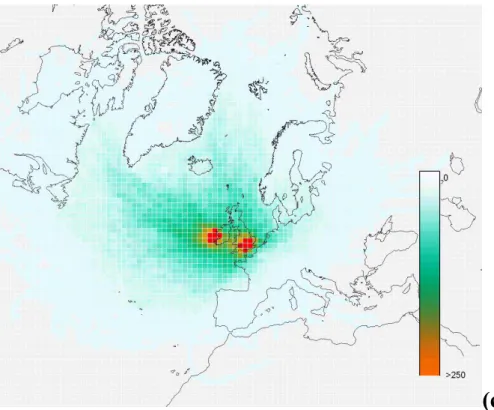
Fig. 9 Solution emission map generated by ES for the enclosing source problem.

Fig. 9. Solution emission map generated by ES for the enclosing source problem.