HAL Id: hal-03236007
https://hal.sorbonne-universite.fr/hal-03236007
Submitted on 26 May 2021
HAL is a multi-disciplinary open access
archive for the deposit and dissemination of
sci-entific research documents, whether they are
pub-lished or not. The documents may come from
teaching and research institutions in France or
abroad, or from public or private research centers.
L’archive ouverte pluridisciplinaire HAL, est
destinée au dépôt et à la diffusion de documents
scientifiques de niveau recherche, publiés ou non,
émanant des établissements d’enseignement et de
recherche français ou étrangers, des laboratoires
publics ou privés.
Y. Lee, A. García Muñoz, A. Yamazaki, M. Yamada, S. Watanabe, T.
Encrenaz
To cite this version:
Y. Lee, A. García Muñoz, A. Yamazaki, M. Yamada, S. Watanabe, et al.. Investigation of UV
Absorbers on Venus Using the 283 and 365 nm Phase Curves Obtained From Akatsuki. Geophysical
Research Letters, American Geophysical Union, 2021, 48 (7), �10.1029/2020gl090577�. �hal-03236007�
1. Introduction
The 80% of solar energy incident on Venus is reflected back to space by the thick and highly reflective clouds that cover the entire planet (Moroz et al., 1985; Tomasko, Smith, et al., 1980). This reflected radiation has a strong directional dependency, which has been used to retrieve the microphysical properties of the cloud aerosols (Arking & Potter, 1968; García Muñoz et al., 2014; Lee et al., 2017; Mallama et al., 2006; Mark-iewicz et al., 2014; Petrova et al., 2015; Shalygina et al., 2015). The reflectivity of Venus is high at visible wavelengths and starts to decrease from the blue toward the ultraviolet (UV) (Barker et al., 1975). The ab-sorption is caused by the SO2 gas at λ < 320 nm (Esposito, 1980; Marcq et al., 2020; Zasova et al., 1981) and
an unidentified secondary absorber (Pollack et al., 1980; Zasova et al., 1981). The latter is usually referred to as the “unknown absorber” (Titov et al., 2018) (hereafter, “UA”). The UA is reported to have its maximum absorption at 340 nm (Pérez-Hoyos et al., 2018) and becomes less absorbing toward shorter wavelengths (Marcq et al., 2020; Pérez-Hoyos et al., 2018), where it overlaps with SO2 absorption.
Abstract
The so-called unknown absorber in the clouds of Venus is an important absorber of solar energy, but its vertical distribution remains poorly quantified. We analyze the 283 and 365 nm phase curves of the disk-integrated albedo measured by Akatsuki. Based on our models, we find that the unknown absorber can exist either well mixed over the entire upper cloud or within a thin layer. The necessary condition to explain the 365 nm phase curve is that the unknown absorber must absorb efficiently within the cloud scale height immediately below the cloud top. Using this constraint, we attempt to extract the SO2 abundance from the 283 nm phase curve. However, we cannot disentangle theabsorption by SO2 and by the unknown absorber. Considering previous SO2 abundance measurements at
midinfrared wavelengths, the required absorption coefficient of the unknown absorber at 283 nm must be more than twice that at 365 nm.
Plain Language Summary
There is an unknown absorber in the clouds of Venus. It absorbs solar energy effectively at ultraviolet (UV) and blue wavelengths, but its vertical location, either above or below the cloud top level (about 70 km altitude), remains unclear. This uncertainty affects our understanding of the vertical deposition of solar energy in the atmosphere. We investigate the vertical distribution of the unknown absorber using the dependence of the full-disk brightness on the scattering direction (the Sun-Venus-spacecraft angle) at 365 nm, with data from JAXA's Akatsuki spacecraft over 3 years. We find that the unknown absorber could exist in the entire cloud, or as a thin layer near but below the cloud top. Using these constraints on the vertical distribution of the unknown absorber, we analyze the 283 nm full-disk brightness. At this shorter wavelength, the SO2 gas and the unknownabsorber are both effective absorbers. We attempt to quantify the SO2 abundance, and find that the
brightness dependence on the scattering direction alone is insufficient to separate the contribution from the two absorbers at 283 nm. Further analysis with spectral phase curve observations will better define the SO2 abundance.
© 2021. The Authors.
This is an open access article under the terms of the Creative Commons Attribution License, which permits use, distribution and reproduction in any medium, provided the original work is properly cited.
Investigation of UV Absorbers on Venus Using the 283
and 365 nm Phase Curves Obtained From Akatsuki
Y. J. Lee1 , A. García Muñoz2 , A. Yamazaki3,4 , M. Yamada5, S. Watanabe6 , andT. Encrenaz7
1Zentrum für Astronomie und Astrophysik, Technische Universität Berlin, Berlin, Germany, 2AIM, CEA, CNRS,
Université Paris-Saclay, Université de Paris, Gif-sur-Yvette, France, 3Institute of Space and Astronautical Science (ISAS/
JAXA), Sagamihara, Japan, 4Graduate School of Science, University of Tokyo, Tokyo, Japan, 5Planetary Exploration
Research Center (PERC), Narashino, Japan, 6Space Information Center, Hokkaido Information University, Ebetsu,
Japan, 7LESIA, Observatoire de Paris, PSL University, CNRS, Sorbonne Université, Université de Paris, Meudon, France
Key Points:
• The vertical distribution of the unknown absorber is investigated with the aid of full-disk phase curves at wavelengths of 283 and 365 nm • First time the 283 nm full-disk
brightness phase curve of Venus is analyzed over a broad phase angle range
• The unknown absorber must result in sufficient absorption within the cloud scale height immediately below the cloud top
Supporting Information:
Supporting Information may be found in the online version of this article.
Correspondence to:
Y. J. Lee,
y.j.lee@astro.physik.tu-berlin.de Citation:
Lee, Y. J., García Muñoz, A., Yamazaki, A., Yamada, M., Watanabe, S., & Encrenaz, T. (2021). Investigation of UV absorbers on Venus using the 283 and 365 nm phase curves obtained from Akatsuki. Geophysical Research Letters, 48, e2020GL090577. https://doi. org/10.1029/2020GL090577
Received 28 AUG 2020 Accepted 8 MAR 2021
10.1029/2020GL090577
The UA is responsible for ∼50% of the solar heating rate at the cloud top level (Crisp, 1986; Lee, Titov, et al., 2015). A recent 365 nm space-based data analysis revealed that the UA abundance has varied by a factor of 2 over the last decade (Lee, Jessup, et al., 2019), showing that such a change in the UA abundance and associated solar heating rate could alter the strength of the Hadley circulation. This may affect the su-per-rotation at the cloud top level atmosphere, explaining the observed long-term variations of wind speeds (Lee, Jessup, et al., 2019).
The vertical distribution of the UA, so far poorly constrained, also affects the solar energy deposition in the atmosphere. Tomasko, Doose, et al. (1980) reported that the solar energy deposition occurred mainly in the upper cloud (>60 km altitude) but not in the middle-to-low cloud (48–60 km). Pollack et al. (1980) and Esposito (1980) argued that the UA is located below the cloud top level to explain the observed phase angle dependence of disk-resolved UV contrasts. Kawabata et al. (1980) concluded from their polarimetric data that the small-size aerosols above the clouds (upper haze) cannot contain the UA. However, Molaver-dikhani et al. (2012) argued for a well-mixed layer of the UA above the cloud top level. Lee, Immamura, et al. (2015) suggested that the vertical distribution of the UA varied over ∼5 years of Venus Express obser-vations. They showed that initially the UA was present above the cloud top but that later was found below. In previous spectral data analyses, the UA has been assumed to be well mixed with the small-size aerosol particles (Marcq et al., 2020; Pérez-Hoyos et al., 2018).
Here, we explore whether the uncertain vertical distribution of the UA may be resolved by analyzing Akat-suki's UV images of the full planetary disk collected over 3 years. We use simultaneous 283 and 365 nm brightness measurements to attempt to extract the absorption of the UA at 283 and 365 nm, and the SO2
abundance. We use ground-based measurements of global mean SO2 abundance (Encrenaz et al., 2019) to
compare and constrain further our findings.
2. Observations
The UV camera (UVI) on board Akatsuki has monitored the Venus dayside since December 2015, acquiring images at 283 and 365 nm (Yamazaki et al., 2018). The Akatsuki spacecraft has a highly elliptical equatorial orbit with an orbital period of ∼10 days (Nakamura et al., 2016). Except for a few hours during pericenter passage, UVI obtains global disk images at a phase angle less than 155°. In this study, we analyzed such full-disk images acquired from December 2015 to January 2019. We rejected images with an insufficient disk coverage within the field-of-view of UVI, for example, when the apparent size of Venus becomes too large, or when the disk location is too off-centered. We also rejected images that contained known artifacts. The total number of selected images are 5,805 at 283 nm and 5,840 at 365 nm; the complete list of them is given by Lee et al. (2020). We calculated the disk-integrated albedo Adisk−int, as the following (Sromovsky
et al., 2001), 2 V S Venus disk int Venus ( ) ( , , ) ( , , ) , Ω ( ) ( ) d t F t A t t S (1)
where λ is the filter's effective wavelength, t is the observation time, α is the Sun-Venus -spacecraft phase angle (°), dV−S(t) is the distance between the Venus and the Sun (AU) at the time of observation t, FVenus(α, λ, t) is the disk-integrated flux of Venus (Wm−2 μm−1), Ω
Venus(t) is the solid angle of Venus as viewed from
Akatsuki, and S⊙(λ) is the solar irradiance at 1 AU (W m−2 μm−1), calculated for the transmittance functions
of each filter. The calculation of Adisk−int is described in the supplementary information (Text S1). A disk−in-t(α = 0°, λ) is the “geometric albedo” at wavelength λ.
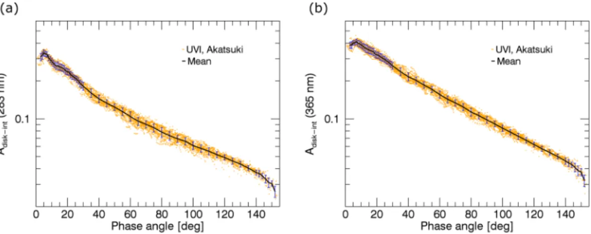
All data points of Adisk−int as a function of α are shown in Figure 1. We also show the mean phase curve over
the 3 years. Short-term variations exist on time scales ranging from a few days to months (Lee et al., 2020), indicated as standard deviations in the same plot. The size of the phase angle bins for the mean phase curve goes from 1° at α < 30° to 5° at 30° ≤ α < 140°, and 2° at α ≥ 140°. This helps capture the glory at small phases (García Muñoz et al., 2014; Lee et al., 2017; Markiewicz et al., 2014), and the decreasing Adisk−int at
Geophysical Research Letters
3. Model Descriptions and Atmospheric Conditions
3.1. Model DescriptionWe fit the observed mean phase curves with model Adisk−int curves obtained by solving the multiple
scat-tering radiative transfer problem with a Preconditioned Backward Monte Carlo (PBMC) algorithm (García Muñoz, 2015; García Muñoz & Mills, 2015). We used a 1 km vertical grid to describe the atmosphere of Ve-nus. We assumed a black surface below the cloud layer (48 km altitude), after confirming that this assump-tion does not change our results and saves calculaassump-tion time (Figure S1). To produce each synthetic phase curve, we used 105 photons, which was deemed a fine balance between calculation efficiency and accuracy.
3.2. Assumed Atmospheric Conditions
We assumed a uniform cloud over the entire disk. The cloud vertical structure above 60 km altitude is reasonably consistent with that used in previous studies, that is, 70 km altitude for the cloud top level (a unity optical thickness, τ = 1, at 365 nm) and 4 km cloud scale height (Figure S2) (Haus et al., 2014; Ig-natiev et al., 2009; Lee et al., 2012; Sato et al., 2020). Two modes of cloud aerosols were assumed: mode 1 with reff = 0.43 μm and νeff = 0.52 (Pollack et al., 1980) and mode 2 with reff = 1.26 μm and νeff = 0.76 (Lee
et al., 2017). The size of mode 2 was inferred from the glory observation of UVI (Lee et al., 2017). We calcu-lated the particles' scattering phase functions using the Lorenz-Mie code by Mishchenko et al. (2002) and a gamma distribution of particle sizes. The refractive indices of 75% H2SO4-H2O cloud aerosols were taken
from Hummel et al. (1988). The cross sections of each mode vary by less than 2% from 365 to 283 nm. This means that the extinction introduced by the mode 1 and mode 2 is effectively the same at both wavelengths investigated here.
The ratio of extinction coefficients of mode 1 and mode 2 was assumed to be 1:1 at 365 nm. In such con-ditions, the particle number density ratio of mode 1 over mode 2 is ∼320 (Figure S2b), according to the ratio of extinction cross sections for mode 1 over mode 2 at 365 nm. This number density ratio is close to the reported ∼400 (Luginin et al., 2016). As smaller ratios were used in other past works (Haus et al., 2014; Pérez-Hoyos et al., 2018), we also explored the impact of a different extinction coefficient ratio, 0.5:1. The resulting differences in brightness are visible at small or large phase angles but not on the overall phase curve shape (Figure S3). Our main conclusions are not very sensitive to the extinction coefficient ratio (Fig-ures 2 and S4) because the UA in our model is considered embedded in both cloud aerosol modes over the specified range of altitudes (Section 3.3). The corresponding extinction coefficient of the aerosols at 283 nm is calculated using the number density and the cross section at 283 nm for each particle mode.
Atmospheric pressure and temperature profiles at low latitudes were taken from Seiff (1983). Rayleigh scat-tering was calculated for the 96.5% CO2 and 3.5% N2 mixture (Sneep & Ubachs, 2005). The absorption cross
10.1029/2020GL090577
Figure 1. Observed disk-integrated albedo at (a) 283 nm and (b) 365 nm as a function of phase angle. Orange dots are
the individual measurements obtained by Akatsuki. Black curves are the mean values. Blue error bars are standard deviations. See the text for details.
section of SO2 was taken from Vandaele et al. (2009) at 283 nm and ignored at 365 nm. We assumed that
the SO2 volume mixing ratio decreases exponentially with altitude with a 3 km scale height (Encrenaz
et al., 2019; Marcq et al., 2020), and adjusted its abundance (ppbv) at the cloud top level. This enables the comparison between our results and those from Encrenaz et al. (2019) in the same manner as done in Marcq et al. (2020). Our prescribed 3 km scale height for the SO2 vertical distribution is somewhat different
from the increasing volume mixing ratio above the cloud top level inferred observationally by Vandaele et al. (2017). We therefore compared the inversion of vertical abundance above the cloud top and a constant SO2 abundance over altitudes (Figure S5b), and found that the three SO2 abundance profiles produced
phase curves with nearly undistinguishable shapes (Figure S5a). Cloud top ozone, localized at high lati-tudes (>50°) (Marcq et al., 2019), is not considered in this study because of the small portion of the high latitudinal area in the fully illuminated equatorial view, 13%, and consequently its small global area aver-aged abundance, ∼1 ppbv.
3.3. Free Model Parameters: SO2 and the UA
In our synthetic phase curve calculations, the vertical distribution of the UA and the abundance of SO2
are described through five free parameters, listed below. We incorporate the UA into the mode 1 and mode 2 particles by reducing the particles' single scattering albedo (SSA), even though in reality both particles absorb negligibly at the two specified wavelengths. This method of reducing the SSA of mode 1 particles to consider the effect of the UA has been used before (e.g., Crisp, 1986). Here, we apply this method for both modes to explore the impact of the vertical distribution of the UA. Thus, in our model we refer to aerosols to mean the combination of mode 1 and mode 2 particles, which include the UA at the prescribed altitude range. The five free parameters are:
• The thickness of the UA layer: ThUA
• The altitude of the UA layer: zUA−cld, which is the middle point between the top boundary altitude of the
UA layer (zUA, top) and the bottom boundary altitude of the UA layer (zUA, bot)
• The ratio of UA absorption relative to aerosol extinction at 365 nm: RUA(365)
• The ratio of UA absorption relative to aerosol extinction at 283 nm: RUA(283)
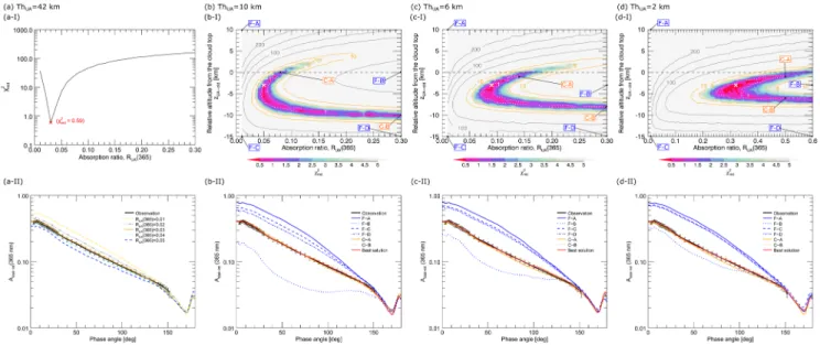
Figure 2. Comparison of the observed and calculated phase curves at 365 nm. ThUA varies from 42 (entire cloud) to 2 km, from left to right columns. The
upper panels show 2
red as a function of RUA(365) (a), and both RUA(365) and zUA−cld (b–d). Note the range of RUA(365) in (d), which is upto 0.6. The dashed lines indicate the cloud top level. The white dotted lines indicate 2
red=1. The area with the values beyond the range of the color bar (2red 5) is filled with light
gray. Orange contours have a different interval than gray contours. The lower panels compare phase curves for selected cases, marked in the upper panels of (b–d): the best solution is for the minimum 2
red (“×”, red2=0.12–0.19), false cases (from F-A to F-D), and comparably good solutions (C-A and C-B). Their exact
conditions and 2
Geophysical Research Letters
• The SO2 abundance in (ppbv) at the cloud topWe experiment with a number of configurations, as follows. (1) ThUA varies from 42 km (entire cloud) to
2 km (thin layer). (2) zUA−cld (also for zUA,top and zUA,bot) varies with respect to the cloud top level, as above +
or below − in steps of 1 km. (3) RUA(365) and (4) RUA(283) define the absorption of UA in terms of a ratio to
the cloud extinction coefficient (km−1). The scattering coefficients for the aerosols become (1 − R
UA
) × Ex-tinction coefficient. Then, the SSA for the cloud aerosols becomes (1 − RUA), that is, SSA = Scattering/
Extinction = (1 − RUA). RUA is nonzero only over the range of altitudes, where the UA is prescribed with (1)
and (2) and we vary RUA in steps of 0.01 to explore its effect. The scattering coefficients of the aerosols and
Rayleigh scattering of the CO2-N2 atmosphere are used to calculate the scattering matrix of the atmosphere
following the usual summation rules. (5) The SO2 abundance is varied in steps of 0.02 in a logarithmic scale,
that is, d(log10(SO2)) = 0.02, from 0.1 to 1,000 ppbv.
We first investigate the phase curve at 365 nm because it is affected by only one active absorber (UA), while there are two active absorbers at 283 nm (UA and SO2). We determine the combinations of ThUA, zUA−cld, and
RUA(365) that are consistent with the observations at 365 nm. After that, with the best fitting configurations
of ThUA and zUA−cld, we attempt to determine RUA(283) and the SO2 abundance at 283 nm.
4. Results
We determine a goodness of fit with a reduced chi-square (2 red):
2 2 red ( 1 1) 1 2 , N i i i i O C N (2)where N is the number of phase angle bins (N = 56), Oi is the mean observed Adisk−int, σi is the associated
standard deviation, Ci is the calculated value, and i denotes each phase angle bin from 3° to 152° (Table S2).
We emphasize that σi is not representative of the signal-to-noise ratio, which is much better than that for
each data point. As seen below, the best fits result in 2
red notably less than one.
4.1. 365 nm Results
We first explore the configuration in which the UA spans the entire cloud (ThUA = 42 km, zUA,top = +20 km,
zUA,bot = −22 km). In this case, the 365 nm phase curve simulation has a single free parameter, RUA(365),
and RUA(365) = 0.03 fits the observation best (red2 =0.59) (Figure 2a). Based on this configuration, we
ex-periment with reducing the top boundary of the UA (zUA,top) from +20 to −10 km. Similarly, we experiment
with increasing the bottom boundary of the UA (zUA, bot) from −22 to +10 km. The resulting red2 contours
(Figures S6a and S6b, respectively) show that a good fit is achieved only when zUA, top ≥ −5 km or zUA, bot < −5 km. We conclude that a vertical distribution of UA extending over the entire upper cloud provides
a satisfactory fit to the observations as long as there is enough UA absorption within 5 km below the cloud top.
We next explore the cases of ThUA ranging from 10 to 2 km (Figures 2b–2d) and thus UA distributions over
layers of varying finite size. For each ThUA, the free parameters are RUA(365) and zUA−cld. The configuration
of minimum 2
red is marked with the “×” symbol in the upper panels (Figure 2I). Selected phase curves are
compared in the lower panels (Figure 2II).
For ThUA = 10 km (Figure 2b) the best solution corresponds to RUA(365) = 0.05 and zUA−cld = −3 km (red2
=0.17). The 2
red 1 area indicates that zUA−cld should be between 0 and −10 km (C-A and C-B) and that the
UA must absorb within the first few kilometers below the cloud top. At zUA−cld = −10 km (UA at 55–65 km),
the sensitivity to RUA(365) becomes weak even for RUA(365) > 0.10 because the UA is located too deep to
have an impact.
For ThUA = 6 km (Figure 2c) the best solution corresponds to RUA(365) = 0.09 and zUA−cld = −3 km (red2
=0.19). The 2red1 area indicates that zUA−cld should be between −1 and −8 km. At zUA−cld = −8 km (UA at
59–65 km), the sensitivity to RUA(365) becomes weak even for RUA(365) > 0.10, as the UA layer reduces its
impact on the planet brightness due to its deep location.
For ThUA = 2 km (Figure 2d) the best solution corresponds to RUA(365) = 0.32 and zUA−cld = −3 km (red2
=0.12). The area of 2
red 1 indicates that zUA−cld should be between −1 and −6 km. At zUA−cld = −6 km (UA
at 63–65 km), the sensitivity to RUA(365) becomes weak even for RUA(365) > 0.40, for the reasons discussed
above.
All our analyses at 365 nm lead to one conclusion: UA absorption within the 5 km below the cloud top is necessary to explain the observed phase curve.
4.2. 283 nm Results
Next, we investigate the 283 nm phase curves. As before, ThUA varies from 42 to 2 km. For ThUA = 2–10 km,
we vary zUA−cld from −1 to −5 that is within the range of good solutions at 365 nm. All results with varying
zUA−cld and ThUA are shown in Figure S8, and Figure 3 shows the results with a fixed zUA−cld = −3 km, which
is the common best solution at 365 nm.
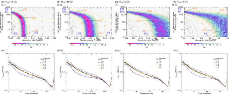
In Figure 3, for each ThUA, the free parameters are RUA(283) and SO2. The red2 contours are shown in the
upper panels (Figure 3I). Selected phase curves are compared in the lower panels (Figure 3II). A degeneracy is seen between the absorption introduced by the UA and SO2 at this wavelength; the SO2 abundance can
be any value below 200–300 ppbv, strongly depending on RUA(283). Similar conclusions are found for the
varying zUA−cld (Figure S8).
Figure 3. Comparison of the observed and calculated phase curves at 283 nm. ThUA varies from 42 (entire cloud) to 2 km, from left to right columns. zUA−cld adopts the best solutions at 365 nm (Panels [b–d], “×”). Other zUA−cld values are used in Figure S8. The upper panels show red2 contours as a function of
RUA(283) and SO2 abundance at the cloud top. Note the range of RUA(283) in (d), which is upto 1.0. The yellow line refers to the reference SO2 abundance, 22.4 ppbv (see the text for details). The white dotted lines indicate 2
red=1. The area with the values beyond the range of the color bar (red2 5) is filled with light
gray. Orange contours have a different interval than gray contours. The lower panels compare phase curves for selected cases as marked in the upper panels:
false cases (from F-A to F-D), and comparably good solutions (from C-A to C-C). Their exact conditions and 2
Geophysical Research Letters
5. Discussion
The observed phase curves result from scattering, mainly by the cloud aerosols, and absorption by SO2
and the UA. As the scattering by the cloud aerosols has a strong phase angle dependence, the effective absorption varies with phase angles especially when it occurs below the cloud top level. In Section 4.1, we showed that this is the case for the UA at 365 nm. We find that the UA could exist in the entire upper cloud or in a thin layer in the cloud, but the necessary condition for all UA scenarios is that sufficient ab-sorption occurs within a few kilometers immediately below the cloud top. So, for any finite depth of UA layer (ThUA = 2–10 km), we find that it must be located near but below the cloud top level. In terms of our
model parameters, this involves that the top of the UA layer (zUA,top) should be, at the deepest, ∼5 km below
the cloud top (Figure S6a and C-B in Figures 2c–2d). Otherwise, the scattering above zUA,top hides the UA
absorption (e.g., F-C and F-D in Figure 2).
For all finite UA layers, all of C-B in Figures 2b–2d are possible solutions at 365 nm, and all of these have zUA,top = −5 km. However, such UA layer with zUA,top = −5 km produces negligible absorption at 283 nm that
is muted in the disk-integrated signal by increased Rayleigh scattering at the shorter wavelengths (2.8 times stronger at 283 nm than at 365 nm) (Figure S7). Such a scenario cannot explain the observed SO2 abundance
that will be discussed later. A similar behavior is also shown in Figure S8cIII. These findings imply that to satisfy the brightness requirements at the two wavelengths, sufficient absorption of the UA should be within one cloud scale height immediately below the cloud top, and that a better fit at 283 nm is achieved when the UA layer is closer to the cloud top level (Figure S8I). We additionally find that zUA,bot < −10 km
(for all other parameters remaining the same) does not affect the phase curves (Figure S6b), implying that our model is only sensitive to altitudes above 60 km (the upper cloud layer).
With the possible solutions of the UA layer at 365 nm, we attempted to constrain the SO2 abundance and
RUA(283). However, we find that the phase angle dependence is insufficient for such a distinction
(Sec-tion 4.2), and that both properties are degenerate in our model even though their prescribed vertical distri-butions are different. To gain insight into this degeneracy, we compare our results with the temporal mean of global SO2 abundance in years 2016–2018, retrieved from midinfrared observations (Encrenaz et al., 2019);
the averaged 450 ppbv at 61 km altitude in 2016–2018 translates into 22.4 ppbv at 70 km with the 3 km scale height of SO2 abundance distribution. Such a SO2 abundance at 70 km in years 2006–2014 showed
a successful consistency between the existent midinfrared and UV observations (Figure 18 in Encrenaz et al. (2019) and Figure 7 in Marcq et al., 2020). So, we expect the same consistency in 2016–2018, and the 22.4 ppbv SO2 is our reference. By doing so, we find the required RUA(283) as 0.07–0.09 (ThUA = 42 km),
0.13–0.14 (ThUA = 10 km), 0.19–0.23 (ThUA = 6 km), and >0.8 (ThUA = 2 km), thereby corresponding to
C-B in Figure 3. These RUA(283) are more than twice RUA(365) for the same ThUA and zUA−cld (Tables S3–S4),
compensating the increased Rayleigh scattering at 283 nm. The required RUA(283) is slightly lower with
zUA−cld = −1 km (Figure S8I) than those with zUA−cld = −3 km (Figure 3), but still RUA(283) > RUA(365) for
all cases. The possible impact of the high-latitudinal ozone would not be an important source of error; its global mean abundance is ∼5% of the SO2 reference, while their absorption cross sections are comparable
at 283 nm (Marcq et al., 2020).
If the increasing absorption of UA from 365 to 283 nm is real, then it would hint at possible UA candidates. We find a similar wavelength dependence of absorption from disulfur dioxide (OSSO) (Wu et al., 2018) and the normal S2O isomer (Frandsen et al., 2020). Wu et al. (2018) measured the absorbance of four types of
OSSO, and showed that it peaks at 287 nm and is therefore stronger than at 365 nm. Frandsen et al. (2020) calculated the absorption cross section of the normal S2O isomer, and showed its peak is near 283 nm,
overlapping with the SO2 absorption peak. Interestingly, these are the two best solutions in Pérez-Hoyos
et al. (2018), although the authors used different absorption spectra for OSSO and S2O from those in Wu
et al. (2018) and Frandsen et al. (2020), respectively. However, our findings on the nature of the UA should be seen as tentative, since we have not explored other possibilities, such as embedding the UA only in mode 1 or mode 2 (but not in both) or different sizes of mode 1 particles. Future analyses with spectral data are necessary to constrain better the UA candidates. We are currently exploring the spectral disk-integrated albedo measurements obtained from the BepiColombo spacecraft during its cruise toward Mercury (Lee, Helbert, et al., 2019). Spectroscopy may allow us to investigate the degeneracy between SO2 and the UA at
nearby wavelengths in the vicinity of 283 nm that are sensitive to different extents to SO2 absorption.
Our phase curve analysis assumes global mean conditions, and we do not investigate latitudinal or lo-cal time variations (e.g., the observed latitudinal variability of the 365 nm brightness is described in Lee et al., 2020). Averaging over 3 years of disk-integrated data should remove most of the variability across the planetary disk. We do not analyze detailed microphysical properties of cloud aerosols, as the current mode 2 size (Lee et al., 2017) explains the glory feature well. Our results provide plausible configurations for the vertical distribution of UA that can be further explored especially for the solar energy deposition calculation which has a considerable impact on the radiative energy balance and the global circulations in the Venusian atmosphere (Lee, Jessup, et al., 2019).
6. Conclusion
We analyzed the disk-integrated phase curves of Venus at 283 and 365 nm in the 3°–152° phase angle range. The observational data over 3 years were acquired by the UV camera on board Akatsuki. We calculated synthetic phase curves with a backward Monte Carlo algorithm to take into account multiple scattering over the full-disk. We explored the 365 nm phase curves with models that incorporate a number of free pa-rameters on the unknown absorber, namely: vertical location and thickness of the unknown absorber layer, and absorption coefficient of the unknown absorber. Our results show that the unknown absorber can exist in the entire upper cloud, or as a thin layer, but it is required that sufficient absorption be present within one cloud scale height immediately below the cloud top. From our analysis at 283 nm, it turns out that we cannot separate absorption by SO2 and the unknown absorber. Comparing our results with the SO2
abun-dance retrieved from the midinfrared observations, we arrive at the tentative conclusion that the absorption coefficient of the unknown absorber at 283 nm is more than twice that at 365 nm. This increased absorption at 283 nm compensates the increased Rayleigh scattering at the same altitudes.
Data Availability Statement
UVI data are publicly available at the JAXA archive website, DARTS (http://darts.isas.jaxa.jp/), and the NASA archive website, PDS (https://pds.nasa.gov/). UVI level 3x products are used in this study, L3bx (doi:10.17597/ISAS.DARTS/VCO-00016, Murakami et al., 2018), and the mean phase curve data are tabu-lated in supplementary Table S2. Processed individual disk-integrated albedo values at 283 and 365 nm are available as supplementary data of Lee et al. (2020).
References
Arking, A., & Potter, J. (1968). The phase curve of Venus and the nature of its clouds. Journal of Atmospheric Science, 25, 617–628. https:// doi.org/10.1175/1520-0469(1968)025<0617:tpcova>2.0.co;2
Barker, E. S., Woodman, J. H., Perry, M. A., Hapke, B. A., & Nelson, R. (1975). Relative spectrophotometry of Venus from 3067 to 5960 Å. Journal of the Atmospheric Sciences, 32, 1205–1211. https://doi.org/10.1175/1520-0469(1975)032<1205:RSOVFT>2.0.CO;2
Crisp, D. (1986). Radiative forcing of the Venus mesosphere. Icarus, 67, 484–514. https://doi.org/10.1016/0019-1035(86)90126-0
Encrenaz, T., Greathouse, T. K., Marcq, E., Sagawa, H., Widemann, T., Bézard, B., et al. (2019). HDO and SO2 thermal mapping on Venus. IV. Statistical analysis of the SO2 plumes. Astronomy and Astrophysics, 623, A70. https://doi.org/10.1051/0004-6361/201833511 Fouchet, L. W. (1980). Ultraviolet contrasts and the absorbers near the Venus cloud tops. Journal of Geophysical Research, 85, 8151–8157.
https://doi.org/10.1029/JA085iA13p08151
Frandsen, B. N., Farahani, S., Vogt, E., Lane, J. R., & Kjaergaard, H. G. (2020). Spectroscopy of OSSO and other sulfur compounds thought to be present in the Venus atmosphere. The Journal of Physical Chemistry A, 124, 7047–7059. https://doi.org/10.1021/acs.jpca.0c04388
García Muñoz, A. (2015). Towards a comprehensive model of Earth's disk-integrated Stokes vector. International Journal of Astrobiology, 14, 379–390. https://doi.org/10.1017/S1473550414000573
García Muñoz, A., & Mills, F. P. (2015). Pre-conditioned backward Monte Carlo solutions to radiative transport in planetary atmospheres. Astronomy and Astrophysics, 573, A72. https://doi.org/10.1051/0004-6361/201424042
García Muñoz, A., Pérez-Hoyos, S., & Sánchez-Lavega, A. (2014). Glory revealed in disk-integrated photometry of Venus. Astronomy and Astrophysics, 566, L1. https://doi.org/10.1051/0004-6361/201423531
Haus, R., Kappel, D., & Arnold, G. (2014). Atmospheric thermal structure and cloud features in the southern hemisphere of Venus as retrieved from VIRTIS/VEX radiation measurements. Icarus, 232, 232–248. https://doi.org/10.1016/j.icarus.2014.01.020
Hummel, J. R., Shettle, E. P., & Longtin, D. R. (1988). A new background stratospheric aerosol model for use in atmospheric radiation models (p. 49). Air Force Geophysics Laboratory, U.S. (Technical rept. No. ADA210110), Scientific Report No.8, AFGL-TR-88-0166
Ignatiev, N. I., Titov, D. V., Piccioni, G., Drossart, P., Markiewicz, W. J., Cottini, V., et al. (2009). Altimetry of the Venus cloud tops from the Venus Express observations. Journal of Geophysical Research, 114. https://doi.org/10.1029/2008JE003320
Lee, Y. J., García Muñoz, A., Imamura, T., Yamada, M., Satoh, T., Yamazaki, A., & Watanabe, S. (2020). Brightness modulations of our nearest terrestrial planet Venus reveal atmospheric super-rotation rather than surface features. Nature Communications, 11, 5720.
https://doi.org/10.1038/s41467-020-19385-6 Acknowledgments
The PBMC algorithm is available upon request to the code author, A. García Muñoz. Y. J. Lee has received funding from EU Horizon 2020 MSCA-IF No. 841432. Open access funding enabled and organized by Projekt DEAL.
Geophysical Research Letters
Lee, Y. J., Helbert, J., Taguchi, M., Murakami, G., Quémerais, E., Watanabe, S., et al. (2019a). 2020 coordinated Venus observations of bepicolombo (ESA and JAXA), Akatsuki (JAXA), and ground-based telescopes. EPSC-DPS joint meeting 2019. Geneva, Switzerland. EPSC-DPS2019-68
Lee, Y. J., Imamura, T., Schröder, S. E., & Marcq, E. (2015a). Long-term variations of the UV contrast on Venus observed by the Venus monitoring camera on board Venus express. Icarus, 253, 1–15. https://doi.org/10.1016/j.icarus.2015.02.015
Lee, Y. J., Jessup, K.-L., Perez-hoyos, S., Titov, D. V., Lebonnois, S., Peralta, J., et al. (2019b). Long-term variations of Venus's 365 nm Albedo observed by Venus express, Akatsuki, MESSENGER, and the Hubble space telescope. The Astronomical Journal, 158, 126. https://doi. org/10.3847/1538-3881/ab3120
Lee, Y. J., Titov, D. V., Ignatiev, N. I., Tellmann, S., Pätzold, M., & Piccioni, G. (2015b). The radiative forcing variability caused by the changes of the upper cloud vertical structure in the Venus mesosphere. Planetary and Space Science, 113–114, 298–308. https://doi. org/10.1016/j.pss.2014.12.006
Lee, Y. J., Titov, D. V., Tellmann, S., Piccialli, A., Ignatiev, N., Pätzold, M., et al. (2012). Vertical structure of the Venus cloud top from the VeRa and VIRTIS observations onboard Venus express. Icarus, 217, 599–609. https://doi.org/10.1016/j.icarus.2011.07.001
Lee, Y. J., Yamazaki, A., Imamura, T., Yamada, M., Watanabe, S., Sato, T. M., et al. (2017). Scattering properties of the Venusian clouds observed by the UV imager on board Akatsuki. The Astronomical Journal, 154, 44. https://doi.org/10.3847/1538-3881/aa78a5
Luginin, M., Fedorova, A., Belyaev, D., Montmessin, F., Wilquet, V., Korablev, O., et al. (2016). Aerosol properties in the upper haze of Venus from SPICAV IR data. Icarus, 277, 154–170. https://doi.org/10.1016/j.icarus.2016.05.008
Mallama, A., Wang, D., & Howard, R. A. (2006). Venus phase function and forward scattering from H2SO4. Icarus, 182, 10–22. https://doi.
org/10.1016/j.icarus.2005.12.014
Marcq, E., Baggio, L., Lefèvre, F., Stolzenbach, A., Montmessin, F., Belyaev, D., et al. (2019). Discovery of cloud top ozone on Venus. Icarus, 319, 491–498. https://doi.org/10.1016/j.icarus.2018.10.006
Marcq, E., Jessup, K.-L., Baggio, L., Encrenaz, T., Lee, Y. J., Montmessin, F., et al. (2020). Climatology of SO2 and UV absorber at Venus' cloud top from SPICAV-UV nadir dataset. Icarus, 335, 113368. https://doi.org/10.1016/j.icarus.2019.07.002
Markiewicz, W. J., Petrova, E., Shalygina, O., Almeida, M., Titov, D. V., Limaye, S. S., et al. (2014). Glory on Venus cloud tops and the un-known UV absorber. Icarus, 234, 200–203. https://doi.org/10.1016/j.icarus.2014.01.030
Mishchenko, M. I., Travis, L. D., & Lacis, A. A. (2002). Scattering, absorption, and emission of light by small particles (p. 445). Cambridge University Press.
Molaverdikhani, K., McGouldrick, K., & Esposito, L. W. (2012). The abundance and vertical distribution of the unknown ultraviolet ab-sorber in the venusian atmosphere from analysis of venus monitoring camera images. Icarus, 217, 648–660. https://doi.org/10.1016/j. icarus.2011.08.008
Moroz, V. I., Ekonomov, A. P., Moshkin, B. E., Revercomb, H. E., Sromovsky, L. A., & Schofield, J. T. (1985). Solar and thermal radiation in the Venus atmosphere. Advances in Space Research, 5, 197–232. https://doi.org/10.1016/0273-1177(85)90202-9
Murakami, S., Ogohara, K., Takagi, M., Kashimura, H., Yamada, M., Kouyama, T., & Imamura, T. (2018). Venus climate orbiter Akatsuki UVI longitude-latitude map data v1.0. JAXA Data Archives and Transmission System. https://doi.org/10.17597/ISAS.DARTS/VCO-00016
Nakamura, M., Imamura, T., Ishii, N., Abe, T., Kawakatsu, Y., Hirose, C., et al. (2016). AKATSUKI returns to Venus. Earth Planets and Space, 68, 75. https://doi.org/10.1186/s40623-016-0457-6
Pérez-Hoyos, S., Sánchez-Lavega, A., García-Muñoz, A., Irwin, P. G. J., Peralta, J., Holsclaw, G., et al. (2018). Venus upper clouds and the UV absorber from MESSENGER/MASCS observations. Journal of Geophysical Research, 123, 145–162. https://doi. org/10.1002/2017JE005406
Petrova, E. V., Shalygina, O. S., & Markiewicz, W. J. (2015). UV contrasts and microphysical properties of the upper clouds of Venus from the UV and NIR VMC/VEx images. Icarus, 260, 190–204. https://doi.org/10.1016/j.icarus.2015.07.015
Pollack, J. B., Toon, O. B., Whitten, R. C., Boese, R., Ragent, B., Tomasko, M., et al. (1980). Distribution and source of the UV absorption in venus' atmosphere. Journal of Geophysical Research, 85, 8141–8150. https://doi.org/10.1029/JA085iA13p08141
Roatsch, K., Coffeen, D. L., Hansen, J. E., Lane, W. A., Sato, M., & Travis, L. D. (1980). Cloud and haze properties from Pioneer Venus polarimetry. Journal of Geophysical Research, 85, 8129–8140. https://doi.org/10.1029/JA085iA13p08129
Sato, T. M., Satoh, T., Sagawa, H., Manago, N., Lee, Y. J., Murakami, S., et al. (2020). Dayside cloud top structure of Venus retrieved from Akatsuki IR2 observations. Icarus, 345, 113682. https://doi.org/10.1016/j.icarus.2020.113682
Seiff, A. (1983). Thermal structure of the atmosphere of Venus. In D. M. Hunten, L. Colin, T. M. Donahue, & V. I. Moroz (Eds.), Venus (pp. 215–279). Tucson, AZ: The University of Arizona Press.
Shalygina, O. S., Petrova, E. V., Markiewicz, W. J., Ignatiev, N. I., & Shalygin, E. V. (2015). Optical properties of the Venus upper clouds from the data obtained by Venus monitoring camera on-board the Venus express. Planetary and Space Science, 113, 135–158. https:// doi.org/10.1016/j.pss.2014.11.012
Sneep, M., & Ubachs, W. (2005). Direct measurement of the Rayleigh scattering cross section in various gases. Journal of Quantitative Spectroscopy and Radiative Transfer, 92, 293–310. https://doi.org/10.1016/j.jqsrt.2004.07.025
Sromovsky, L. A., Fry, P. M., Baines, K. H., & Dowling, T. E. (2001). Coordinated 1996 HST and IRTF Imaging of Neptune and Triton. II. Implications of disk-integrated photometry. Icarus, 149, 435–458. https://doi.org/10.1006/icar.2000.6563
Titov, D. V., Ignatiev, N. I., McGouldrick, K., Wilquet, V., & Wilson, C. F. (2018). Clouds and hazes of Venus. Space Science Reviews, 214, 126. https://doi.org/10.1007/s11214-018-0552-z
Tomasko, M. G., Doose, L. R., Smith, P. H., & Odell, A. P. (1980a). Measurements of the flux of sunlight in the atmosphere of Venus. Journal of Geophysical Research, 85, 8167–8186. https://doi.org/10.1029/JA085iA13p08167
Tomasko, M. G., Smith, P. H., Suomi, V. E., Sromovsky, L. A., Revercomb, H. E., Taylor, F. W., et al. (1980b). The thermal balance of Venus in light of the Pioneer Venus mission. Journal of Geophysical Research, 85, 8187–8199. https://doi.org/10.1029/JA085iA13p08187
Vandaele, A. C., Hermans, C., & Fally, S. (2009). Fourier transform measurements of SO2 absorption cross sections. II. Temperature de-pendence in the 29,000-44,000 cm−1 (227-345 nm) region. Journal of Quantitative Spectroscopy and Radiative Transfer, 110, 2115–2126.
https://doi.org/10.1016/j.jqsrt.2009.05.006
Vandaele, A. C., Korablev, O., Belyaev, D., Chamberlain, S., Evdokimova, D., Encrenaz, T., et al. (2017). Sulfur dioxide in the Venus atmos-phere: I. Vertical distribution and variability. Icarus, 295, 16–33. https://doi.org/10.1016/j.icarus.2017.05.003
Wu, Z., Wan, H., Xu, J., Lu, B., Lu, Y., Eckhardt, A. K., et al. (2018). The near-UV absorber OSSO and its isomers. Chemical Communica-tions, 54, 4517–4520. https://doi.org/10.1039/C8CC00999F
Yamazaki, A., Yamada, M., Lee, Y. J., Watanabe, S., Horinouchi, T., Murakami, S.-y., et al. (2018). Ultraviolet imager on venus orbiter Akatsuki and its initial results. Earth Planets and Space, 70, 23. https://doi.org/10.1186/s40623-017-0772-6
Zasova, L. V., Krasnopolskii, V. A., & Moroz, V. I. (1981). Vertical distribution of SO2 in upper cloud layer of Venus and origin of U.V.-ab-sorption. Advances in Space Research, 1, 13–16. https://doi.org/10.1016/0273-1177(81)90213-1
References From the Supporting Information
Chance, K., & Kurucz, R. L. (2010). An improved high-resolution solar reference spectrum for earth's atmosphere measurements in the ultraviolet, visible, and near infrared. Journal of Quantitative Spectroscopy and Radiative Transfer, 111, 1289–1295. https://doi. org/10.1016/j.jqsrt.2010.01.036
Lee, Y. J., García Muñoz, A., Imamura, T., Yamada, M., Satoh, T., Yamazaki, A., & Watanabe, S. (2020). Brightness modulations of our near-est terrnear-estrial planet Venus reveal atmospheric super-rotation rather than surface features. Nature Communications, 11, 5720. https:// doi.org/10.1038/s41467-020-19385-6
Vandaele, A. C., Korablev, O., Belyaev, D., Chamberlain, S., Evdokimova, D., Encrenaz, T., et al. (2017). Sulfur dioxide in the Venus atmos-phere: I. Vertical distribution and variability. Icarus, 295, 16–33. https://doi.org/10.1016/j.icarus.2017.05.003
Yamazaki, A., Yamada, M., Lee, Y. J., Watanabe, S., Horinouchi, T., Murakami, S.-y., et al. (2018). Ultraviolet imager on venus orbiter Akatsuki and its initial results. Earth Planets and Space, 70, 23. https://doi.org/10.1186/s40623-017-0772-6