Continuum modeling of particle suspension conductivity

Continuum Modeling of Particle Suspension

Conductivity

by

Tyler J. Olsen

Submitted to the Department Mechanical Engineering

in partial fulfillment of the requirements for the degree of

Master of Science in Mechanical Engineering

at the

MASSACHUSETTS INSTITUTE OF TECHNOLOGY

ARCHIVES

MASSACHUSETTS INSTITUTE OF TECHNOLOGY

OCT 01 2015

LIBRARIES

September 2015

@

Massachusetts Institute of Technology 2015.

A uthor ...

Certified by ...

Accepted by...

All rights reserved.

IA

Signature redacted

Department Vechanical Engineering

August 19, 2015

A

/

Signature redacted

I ,

Kenneth N. Kamrin

Assistant Professor

Thesis Supervisor

Signature redacted

David E. Hardt

Ralph E. and Eloise F. Cross Professor in Manufacturing

Chairman, Committee on Graduate Students

Continuum Modeling of Particle Suspension Conductivity

by

Tyler J. Olsen

Submitted to the Department Mechanical Engineering on August 19, 2015, in partial fulfillment of the

requirements for the degree of

Master of Science in Mechanical Engineering

Abstract

A suspension of network-forming, electrically conductive particles imparts electrical conductivity to an otherwise insulating medium. This effect can be used to great effect in many industrial applications. The ability to describe these networks and to predict their physical properties is a key step in designing systems that rely on these properties. In addition, many times these networks are suspended in a flowing fluid, which disrupts existing networks and forms new ones. The extra layer of complexity introduced by flow requires more sophisticated tools to model the effect on the network and its properties.

In the first chapter, we derive a model for the full, tensorial effective conductivity of a particle particle network as a function of a local tensor description of the par-ticle network, the "fabric tensor." We validate our model against a large number of computer-generated networks and compare its performance against an analogous existing model in the literature. We show that the model accurately predicts the isotropic magnitude, deviatoric magnitude, and deviatoric direction of a particle net-work.

In the second chapter, we set out to model the effects of flow on a particle network. We propose two frame-indifferent constitutive equations for the evolution of the fabric tensor. We perform conductivity measurements of real flowing carbon black suspen-sions and fit our models to the results by using the conductivity model derived in chapter 1. We find that our models are able to reproduce out-of-sample experimental results with a high degree of accuracy.

Thesis Supervisor: Kenneth N. Kamrin Title: Assistant Professor

Acknowledgments

First and foremost, I would like to thank my advisor Professor Ken Kamrin for his support, mentorship, and (seemingly infinite) patience. His enthusiasm, knowledge, and experience have been invaluable throughout the course of this work. I am excited to be able to continue my work as a Ph.D. candidate under his guidance.

I would also like to thank my labmates Sachith, Ramin, Hesam, Patrick, Chen-Hung, Qiong, and Jake. I couldn't imagine a better group of colleagues with whom to be down in the trenches.

Last, and certainly not least, I would like to thank my wife Sarah. She is always there pushing me when I become complacent, motivating me when I get discouraged, and cooking dinner when I get too caught up in work to feed myself.

Contents

1 Modeling Tensorial Conductivity of Particle Suspension 1.1 Summary ... ...

1.2 Introduction . . . .. . . . . 1.3 Homogenization . . . . 1.4 Lattice-Reduced Model . . . . 1.5 Numerical Simulation . . . . 1.5.1 Aside: Packing dependence on diffusion . . . . 1.6 T ests . . . . 1.7 Discussion and Conclusions . . . . 1.8 Acknowledgements . . . .

2 Suspension Microstructure Evolution

2.1 Introduction . . . . 2.1.1 Necessary Background . . . . 2.2 Evolution Law . . . . 2.2.1 Specialization of Constitutive Equation . . . . 2.3 M ethods . . . . 2.3.1 Experimental Setup . . . . 2.3.2 Experiments Performed . . . . 2.3.3 Model Fitting . . . . 2.4 R esults . . . . 2.4.1 Linear Model . . . . Networks 15 15 16 18 22 26 29 32 36 38 39 39 40 41 43 52 53 54 54 57 57

2.4.2 Nonlinear Model . . . . 2.5 Discussion and Conclusions . . . . 2.5.1 Future W ork . . . . 2.6 Acknowledgements . . . .

A Selected Source Code: nparticle.cpp

B Selected Source Code: fitsteadyState nonlinear.m

63 69 71 71 73 85

List of Figures

1-1 (a) Image of a carbon black particle network, an electrically conductive suspension

[241.

(b) Image of an effective two-dimenionsional suspen-sion (attractive polystyrene beads on a fluid surface), which has been subjected to shearing. Note the formation of an anisotropic contact network between particles. 1251 . . . . 18 1-2 Schematic of a small resistor network with nodes and edges labeled

according to our conventions. . . . . 21 1-3 Schematic of particles in contact showing contact vectors n(.. .... 21 1-4 Idealized particle lattice and unit cell from which fabric-conductivity

relation was derived. (a) Example 2D idealized particle lattice. (b) 2D lattice unit cell and its resistor network analog. Neighboring unit cells are shown in gray dashed lines. . . . . 23 1-5 Example (using a small number of particles) of a dense particle packing

resulting from Algorithm 1.1. . . . . 27 1-6 Example (using a small number of particles) of a packing resulting

from Algorithm 1.2 using a small number of particles. . . . . 29 1-7 Packing volume fraction resulting from algorithm 1.2 as a function of

F . . . . 30

1-8 Example 10,000-particle packing (from Algorithm 2) with its associated

1-9 Predicted relationship between the (modified) trace of the conductivity and the fabric trace, compared to numerical results of 50,000 packings generated by Algorithm 1 and 10,000 generated under Algorithm 2. Inset is a zoom-in of the vicinity of trA = 2. . . . . 34 1-10 Predicted relationship between effective magnitude of the anisotropy

of the conductivity and the invariants of the fabric. Error bars show one standard deviation. . . . . 35 1-11 PDF of angle differences are distributed around zero, indicating

codi-rectionality of the fabric and conductivity tensors, as predicted by the analytical model, i.e. (1.16). . . . . 36 1-12 Plot of the relative error of the trace of conductivity. (Left) Relative

error from packings created with Algorithm 1.1. (Right) Relative error from packings created with Algorithm 1.2. . . . . 37 1-13 Plot of the relative error of the determinant of conductivity. (Left)

Rel-ative error from packings created with Algorithm 1.1. (Right) RelRel-ative error from packings created with Algorithm 1.2. . . . . 37

2-1 Schematic of particles in contact showing contact vectors n('). ... 40 2-2 Log-log plot of trA, - trA vs time shows power-law nature of trA

decay to steady state. . . . . 51

2-3 Schematic of device used to perform rheo-electric measurements. . . . 53

2-4 Linear Model fit of steady-state current measurements at different nom-inal shear rates. . . . . 58 2-5 Linear Model prediction of steady-state transverse conductivity as a

function of shear rate in simple shear. . . . . 59 2-6 Linear Model prediction of normalized current as a function of time

during 30 second ramp experiment with 0s = 5s- and ':2) = 100s-. 61

2-7 Linear Model prediction of normalized current as a function of time during 60 second ramp experiment with s1 = 50s-1 and 2y = 100s-. 61

2-8 Linear Model prediction of normalized current as a function of time during 300 second ramp experiment with '1 50s-1 and 2= 100s-. 62 2-9 Linear Model prediction of normalized current as a function of time

during 30 second ramp experiment with A1 50s-1 and A2 =200s-1. 62

2-10 Linear Model prediction of normalized current as a function of time

during 60 second ramp experiment with '1 = 50s-1 and Y2 = 200s-1. 63

2-11 Linear Model prediction of normalized current as a function of time during 300 second ramp experiment with A1 50s-1 and Y2 - 200s . 63 2-12 Nonlinear Model fit of steady-state current measurements at different

nominal shear rates. . . . . 65 2-13 Nonlinear Model prediction of steady-state transverse conductivity as

a function of shear rate in simple shear. . . . . 65 2-14 Nonlinear Model prediction of normalized current as a function of time

during 30 second ramp experiment with 1 50s1 and A2= 100s-1. 66 2-15 Nonlinear Model prediction of normalized current as a function of time

during 60 second ramp experiment with A1 50s-1 and 2= 100s-1. 67 2-16 Nonlinear Model prediction of normalized current as a function of time

during 300 second ramp experiment with 1 = 50s-1 and '2 = 100s-1. 67

2-17 Nonlinear Model prediction of normalized current as a function of time during 30 second ramp experiment with '1 = 50s- and 12 = 200s-. 68

2-18 Nonlinear Model prediction of normalized current as a function of time

during 60 second ramp experiment with A₁ 50s-1 and A2 - 200s-1 68

2-19 Nonlinear Model prediction of normalized current as a function of time

List of Tables

2.1 Parameters used to fit the Linear Model to the experimental data 58 2.2 Parameter sets for the transient ramp experiments . . . .. . . . 60 2.3 Parameters used to fit the Nonlinear Model to the experimental data 64

Chapter 1

Modeling Tensorial Conductivity of

Particle Suspension Networks

Chapter 1 largely appeared in a publication by Olsen and Kamrin

[34].

The chapter here contains additional details.

1.1

Summary

Significant microstructural anisotropy is known to develop during shearing flow of attractive particle suspensions. These suspensions, and their capacity to form con-ductive networks, play a key role in flow-battery technology, among other applica-tions. Herein, we present and test an analytical model for the tensorial conductivity of attractive particle suspensions. The model utilizes the mean fabric of the network to characterize the structure, and the relationship to the conductivity is inspired by a lattice argument. We test the accuracy of our model against a large number of computer-generated suspension networks, based on multiple in-house generation pro-tocols, giving rise to particle networks that emulate the physical system. The model is shown to adequately capture the tensorial conductivity, both in terms of its invariants

and its mean directionality.

1.2

Introduction

The electrical conductivity of heterogeneous materials has been extensively studied by many different researchers over the years [5, 11, 44, 42, 261. The literature primarily focuses on heterogeneous materials which are mixtures of two materials that each have different, isotropic electrical conductivities. The most well-known result is that of Maxwell, which is based on an effective-medium approximation for dilute suspensions

[301. Hashin and Shtrikman approached the problem in a different way. Rather than attempt to solve for an exact expression for the effective conductivity of a randomly structured material, they applied a variational method to derive upper and lower bounds on the effective conductivity [221. They chose to use a variational approach to derive bounds on the conductivity because solving the exact problem for an arbitrarily structured heterogeneous material was analytically intractable. Torquato

[44,

42, 43] has studied the effective conductivity problem in great depth. He has improved the bounds laid out by Hashin and Shtrikman, has solved for effective conductivity of a number of different lattice types, and has expressed the exact tensorial effective conductivity in terms of an infinite series of N-point probability functions, which can be used to describe the microstructure of a heterogeneous material. The particular case of a suspension consisting of a conductive particle network within an insulating medium has been considered theoretically, to our knowledge, in one existing study [26]. The approach they take assumes a spatially homogeneous potential gradient field imposed upon the structure, leading to a model for the conductivity that can be proven to be an upper bound.

Much of the aforementioned work is concerned with the isotropic conductivity of het-erogeneous materials. In this work, we aim to model the full tensorial conductivity, with a focus on suspended networks of conductive particles. These particle networks are of practical importance, especially in flowable battery technology currently

un-der development by the Joint Center for Energy Storage Research (JCESR)

1141.

In these batteries, a conductive, flowing suspension of carbon black forms an integral component of the system, see Figure 1-1(a). It has been shown in related systems 1251 that shearing flows induce anisotropy in a contact network of suspended particles, as pictured in Figure 1-1(b). In instances where suspension conductivity arises from particle-particle contacts, this structure anisotropy should give rise to conductivity anisotropy. It is this behavior that we seek to describe. It has been shown experi-mentally that the electrical conductivity of a suspension is highly sensitive to shear rate[2], dropping by several orders of magnitude as shear rate increases. From this observation and the evidence of particle microstructure changing in shearing flow, we deduce that a suitably chosen description of the particle network should be sufficient to predict the electrical conductivity of a suspension.

In the granular media literature, a great deal of attention has been given to describ-ing the structure of the contact network between particles. Perhaps the simplest structural measure for such a network that includes anisotropy is the fabric ten-sor

[33,

31, 371. While more complex structural measures exist, such as pair- and higher-order particle correlation functions[44], whose use could enable greater accu-racy in constructing a conductivity model, we shall show that a suitable model can be achieved solely in terms of the fabric. Key to our model development is the so-lution of a simple case, based on a network conforming to a lattice structure. The results instruct the form for a new conductivity model, whose accuracy is then tested against many thousands of random particle networks. To explore a range of particle networks, we describe two distinct algorithms for creating random packings - one for denser packings, and one for more dilute packings that closely resemble those formed by carbon-black - and demonstrate the model's predictive capability against thousands of packings generated from both algorithms.

(a) (b)

Figure 1-1: (a) Image of a carbon black particle network, an electrically conductive suspension

[24].

(b) Image of an effective two-dimenionsional suspension (attractive polystyrene beads on a fluid surface), which has been subjected to shearing. Note the formation of an anisotropic contact network between particles.

[251

1.3

Homogenization

The tensorial form of Ohm's law relates the electric field vector E to the current density vector J through a second-order conductivity tensor K, i.e.

J=KE (1.1)

The conductivity tensor is a symmetric, positive-definite tensor

[431.

An effective con-ductivity for a representative volume Q of a heterogeneous material must be defined prior to any analytical or numerical work. The effective conductivity of an ergodic medium is defined by

(J) = K(E) (1.2)

where

(E)

and (J) are, respectively, the spatially-averaged electric and current density fields over Q

[431.

To avoid a possibly overreaching assumption of ergodicity -our tests will be conducted on finite domains - we specify that (E) is imposed by prescribing a linear boundary potential p(x E &Q) = -(E) -x, and that (J) is redefined as the flux that is power-conjugate to

KE).

That is,

where

j

is the local current density field. In the ergodic limit of the ensuing analysis, (J) reduces to a standard spatial average.

Assuming that the current density obeys Kirchoff's current law and Ohm's law -respectively, V -

j

= 0 and

j

= -aVp for some non-negative conductivity field U(x) - a symmetric, positive-definite conductivity tensor K must exist that obeys (1.2). By using the divergence theorem, Eq 1.3 can be transformed into

(E) - K (E) = J -Pj-ndA (1.4) aQ

where n is the outward-pointing normal vector.

We model the particles as perfect conductors, the fluid as a perfect insulator, and we suppose electrical resistance arises only at the contacts between particles. Likewise, the field o is approximated as a constant within each particle but possibly varying from particle to particle. The above integral can now be broken into a sum of integrals over the boundary. In the locations where the boundary passes through free space (i.e., not a particle), then we know that

j

is exactly 0. This leaves only the parts of the boundary that pass through particles, which allows us to write the integral over the set of boundary particles B, i.e.

(E) -K(E) = O

j

-n dA. (1.5)

iCB

where Qj is the intersection of the ith boundary particle with 0Q, and the potential within particle i, denoted vo above, can be brought outside the integral since it is constant within a particle. Although the precise nature of

j

is unknown within the particle, the value of the integral faa

j

- n dA is the current that is flowing out of Q. Denoting this current as Iu' we can write the final expression for the right-hand-side of (1.4),

(E) -K(E) = - ojI""t. (1.6) V iB

The three independent components of Ke can be determined by performing multiple simulations on the same particle network with three non-colinear choices of

(E).

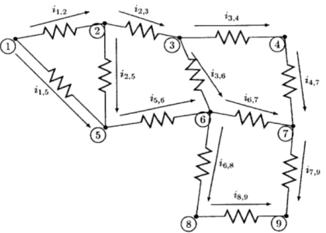
By our assumptions for the particle properties, the problem can be reduced further to that of a resistor network. The network is defined by the set of particles acting as the nodes, which are connected by a set of contacts acting as the edges, which carry a resistance R,. In our model development and simulations, we assume that R, is a constant at all contacts. In reality, this is not strictly the case since the contact resistance is affected by the contact area between particles and the local structure of the network. This was studied in detail by Batchelor[6. If the particles in question were Hertzian elastic spheres compressed into a dense granular packing, spatially-fluctuating contact forces arise causing spatially-fluctuating contact areas, and this issue may be a factor to consider. However, for the suspensions of interest in this study, the particles actually have an open, fractal structure, and form contacts only due to van der Waals attraction. Absent any information to inform the size of the contact area beside the ~ constant attractive force, we choose to use a constant contact resistance. A schematic of an example network with 9 nodes and 12 edges can be found in figure 1-2. Supposing an N-particle sample and letting i represent the (signed) current flowing from particle m to n, Ohm's and Kirchoff's law can be rewritten in their simpler discrete form,

_, P - H nPm (1.7)

and

irn = 0 for all m. (1.8)

where Hmn is the adjacency matrix of the graph formed by the particle network.

Hmnn = 1 if there is an edge connecting particles m and n, and zero otherwise. These

equations define a sparse linear system that can be solved for the potential at each

particle after applying appropriate boundary conditions, which is described in a later

section. The resulting linear system is sparse, symmetric, and positive definite, so we used a sparse Cholesky direct solver to compute the potential at each point. A trivial

28,9

Figure 1-2: Schematic of a small resistor network with nodes and edges labeled ac-cording to our conventions.

3.

Figure 1-3: Schematic of particles in contact showing contact vectors n(/).

post-processing step can be performed to compute the current through each contact. Solving these linear equations for a given particle network enables us to calculate I'"* in (1.6) and hence the conductivity tensor for the network.

We choose to use the fabric tensor as the measure of the network structure. The particle-level fabric is a local quantity that can be defined for particle p by the relation

[37, 33, 311

where 0 denotes the dyadic product, and n is the unit vector connecting particle centroids of the i'th contact on the particle. This is illustrated in Figure 1-3. To homogenize over the entire particle network, or at least meso-sized region of it, the average fabric tensor is defined as the system average of the particle fabric tensors.

l fNparticnes

A- =( A (1.10)

The definition of the fabric tensor has some attractive features. It is symmetric and positive-semidefinite, guaranteeing that the eigenvalues are non-negative and that the eigenvectors are orthogonal. These properties are shared by the conductivity tensor K, suggesting the fabric tensor could be an appropriate independent variable in the conductivity's functional form.

An important concept that will be used later is that of a tensor deviator. The tensor deviator is the trace-free part of a tensor, and it is useful to describe anisotropic phenomena since it has the isotropic part removed. It is defined as

1

Ao = -A - -trA 1 (1.11)

d

where d is the spatial dimension and 1 is the identity tensor.

1.4

Lattice-Reduced Model

We propose an analytical model to elucidate the connection between electrical con-ductivity and the fabric tensor based on a simplified lattice structure. We will test this model's applicability to random packings in the later sections.

The particles are imagined to live on an idealized infinite, periodic lattice. The lattice is parameterized by a set of numbers that describe the particle size and spacing. These parameters are (1) particle diameter D,, (2) distance in x-direction between chains do, (3) distance in y-direction between chains dy, (4) distance in z-direction between chains d,. In 2D, only the first three parameters are used. An illustration of a 2D lattice characterized by these parameters is shown in figure 1-4(a), with its fundamental unit cell shown in figure 1-4(b).

Both the average fabric tensor and effective conductivity can be computed analyti-cally. The average fabric tensor is defined as the spatial average of the fabric tensor

(a)

dy

DP

dX

(b)

Figure 1-4: Idealized particle lattice and unit cell from which fabric-conductivity relation was derived. (a) Example 2D idealized particle lattice. (b) 2D lattice unit cell and its resistor network analog. Neighboring unit cells are shown in gray dashed lines.

for all of the particles in the unit cell and ultimately results in the formua

A = (1.12)

N + NY- _{o NY}

In this expression, the key quantities to recognize are the number of particles in the x-oriented chain, Nx = d

/Dp,

and the number of particles in the y-oriented chain,

N -= dy/Dp.

Next, the effective conductivity was derived for the unit cell. To do this, imagine applying an arbitrary voltage difference across the x-oriented and y-oriented chains separately. These voltages are Ay2 and Amy, respectively. By applying Ohm's law through the corresponding chains, we can recover the components of the vector form

of Ohm's Law shown in (1.1). For example, for the x-oriented chain

j. = - ((VpX (1.13)

with (Vo)x = Agx/dx. Due to the geometry of the problem, we know that the off-diagonal components of the conductivity tensor K are exactly zero. Therefore, we can say

K1 . (1.14)

Similarly analysis yields

1

K22 = . (1.15)

Finally, the parameters Nx and N. can be algebraically eliminated to give the com-ponents of K in terms of the comcom-ponents of A, yielding the tensorial relationship

1 trA - 2

K =A. (1.16)

R, det A

We refer to the formula in (1.16) as the "lattice model". A similar analysis can be carried out for a three-dimensional unit cell, which will yield the following expression for the conductivity tensor,

K 1 (trA - 2)2A (1.17)

4DPRC det A

The formulae above apply when trA-2 is non-negative. Otherwise the solution is K 0. The matrix A/ det A can be understood as an approximate measure of how much a lattice cell of given perimeter (area) deviates from a square (cube) configuration, distributing proportionally less conductivity in directions where particle chains are more separated and more conductivity in directions where chains are tightly spaced.

Despite its inspiration from the lattice structure, there are several reasons to consider the applicability of the lattice model to more general particle networks. For one, the formula purports codirectionality of the fabric and conductivity, i.e. the deviators

of the two tensors are aligned, implying that the direction of anisotropy of one ten-sor gives the anisotropy direction of the other, which to a first approximation ought to match the behavior of general particle networks. Second, the results imply that conductivity should vanish when trA < 2, which is sensible more generally (though not strictly) because particles in a percolating chain, as needed to conduct current across the sample, must have coordination number at least two. Above this thresh-old, conductivity increases with trA in line with one's basic intuition for more highly coordinated networks. In reality, islands of monomers, dimers, etc, enable the pos-sibility of conductivity with an average coordination number less than two because conductivity will be nonzero with any percolating chain of particles. However, the ge-ometric assumption underlying this lattice model prevents this from being taken into consideration. This shortcoming of the model is evident in our numerical results in figure 1-9 where nonzero conductivity was observed for a small range of coordination

numbers below two.

We are aware of one other fabric-based analytical model for conductive particle net-works, which was developed by Jagota and Hui [26]. In their work, a uniformity hypothesis is made with regard to the potential gradient, which results in a conduc-tivity model that is fully linear in the fabric tensor,

Nv, D2

K = A. (1.18)

2 Re

The above, which can be proven to be an upper-bound on the real conductivity, is for a two-dimensional system and NV is the particle number fraction (per area in 2D). In the isotropic case, (1.18) reduces to precisely the Hashin-Shtrikman upper bound

one finds for the limit of thin, conductive bridges (of net resistance R,) connecting the centers of contacting particles [22, 431. The above model differs from ours most notably in that the conductivity is not thresholded by the coordination number, the formula depends explicitly on the particle area fraction as well fabric, and it does not depend on the fabric determinant.

1.5

Numerical Simulation

In order to perform numerical experiments and determine the generality of the lattice model, a large number of random particle networks (packings) must be created. There are a number of methods to do this already in the granular and particulate matter literature. See the references for a broad summary of the currently available granular packing algorithms[4]. Attractive suspensions have been modeled with the Diffusion-Limited Aggregation (DLA) model of Witten and Sander[271. A common feature of

many of the granular statics methods is that they solve force equilibrium equations for a system of particles This was not a feature that was required for this study, so these types of methods were not used, in the interest of saving computational time. Instead, we developed two methods for creating two-dimensional random contact networks of particles, and we tested our model against numerous packings generated by each method. Both methods allow us to influence the resulting anisotropic structure of the packings.

Algorithm 1: Our first packing algorithm was designed to create a dense random contact networks of particles. This is in contrast to a later algorithm, to be described below, which created packings that resulted in much lower-density packings. The dense packings were created by perturbing a 2D hexagonal close-packing of particles. This was achieved by placing points into a triangular lattice, adding random noise to the position of each point, and finally growing each particle as large as possible such that no particles overlapped. Anisotropy can be influenced by shearing the points with an affine transformation x' =F x before growing the radii. This process is described in pseudocode below (Algorithm 1.1). An example of the resulting packing overlaid by its analogous resistor network is shown in figure 1-5.

Figure 1-5: Example (using a small number of particles) of a dense particle packing resulting from Algorithm 1.1.

Algorithm 1.1

Seed L x L box with close-packed points Perturb points with random noise

Move each point to new location x' by x' = F x while Not all radii frozen do

Find smallest distance that any particle can grow Grow all particles by this amount

Freeze radii of particles that come into contact end while

Algorithm 2: This procedure was motivated by a need to better understand the con-ductivity of carbon black suspensions in an insulating medium. The self-attraction carbon black particles leads to fractal particle networks that are electrically percolat-ing at low volume fraction (below 1 vol%)114].

To produce structures that more closely resemble carbon black suspensions, we devel-oped our second packing algorithm, which is inspired by the "hit-and-stick" behavior of the carbon particles. In addition, the new algorithm is able to include the effects of particle Brownian motion but this is not essential to the algorithm.

d is the number of spatial dimensions. Next, a linear velocity field is imposed directly

on each cluster's centroid according to

v = -B(x - O)+ VB (1.19)

where 0 is a point in the middle of the original box. This imposed velocity field serves to pull all of the clusters together. The extra term, VB, is a random velocity

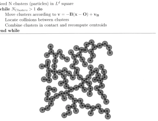
due to Brownian motion. The magnitude of this term can be tuned at runtime. The matrix B is a d x d matrix that allows us to impose an anisotropic velocity field. This allows us to influence (but not completely impose) the fabric tensor that results from this packing method. After the velocity field is imposed, the particle positions are updated by assuming a time step dt (computed at runtime). Then, the clusters are checked to determine whether any contacts have been made with other clusters. If so, the clusters are cohered into a single cluster for all future steps. This process of imposing velocity, updating positions, and handling contacts is repeated until only a single cluster remains. The process is outlined in pseudocode in Algorithm 1.2. An example of a packing resulting from this process is shown in figure 1-6 and a larger example is displayed in figure 1-8.

The box-counting fractal dimension [161 of the resulting packings was computed in order to determine if they resembled real-life packings found in experiments. The fractal dimension of packings produced by this method is approximately d = 1.75. This was compared against the particle network image in figure 1-1. This network has a fractal dimension of approximately d = 1.7 0.1. Uncertainty in the mea-surement is due to the image processing techniques used to identify particles. Based on these measurements, we are satisfied that this algorithm produces realistic pack-ings, although more detailed correlation function measurements would be needed for a firmer conclusion.

Algorithm 1.2

Seed N clusters (particles) in L' square

while Natiters > 1 do

Move clusters according to v = -B(x - 0) + VB

Locate collisions between clusters

Combine clusters in contact and recompute centroids end while

Figure 1-6: Example (using a small number of particles) of a packing resulting from Algorithm 1.2 using a small number of particles.

1.5.1

Aside: Packing dependence on diffusion

While using algorithm 1.2, we noticed that the strength of the diffusion term vB had

a large impact on the final volume fraction of the resulting packing. To explore this effect in more detail, we defined a non-negative dimensionless parameter F, jokingly

called the "fluffy factor." F is defined as

D

F = (1.20)

where D is the standard diffusion coefficient for Brownian motion. By examining the definition of F, we see that F = 0 corresponds to pure advection by the sink defined by B, and F - oo corresponds to the case of pure diffusion. We then performed a series

0.25 c 0.2 0 0.15 -0 (I) 0.15 .5-0 0 2 4 6 8 10 Fluffy Factor

Figure 1-7: Packing volume fraction resulting from algorithm 1.2 as a function of F.

of 10000 three-dimensional simulations spanning F C [010]. The resulting volume

fractions were binned by F value and plotted in figure 1-7. The plot shows that the average volume fraction of a packing decreases with F. Additionally, the deviation from the mean behavior is extremely small, on the order of 0.5%, indicating that F is strongly predictive of the volume fraction of a packing.

The utility of this observation rests in the one-to-one correspondence of F and packing

fraction. It provides a means of observing an existing packing and inferring the

strength of diffusion relative to advection during the formation of the packing. This could, for example, provide some insight into the presence of flow during the formation of a packing of particles for which the diffusion constant is known. Similarly, it can provide an estimate of the diffusion coefficient if the flow conditions during packing formation are known. However it can be used, it is an interesting relationship that merits further study at a later time.

Applying boundary conditions: In order to apply the solution method described above

to an arbitrary packing of particles, appropriate boundary conditions must be applied. In these simulations, a prescribed voltage was applied to particles all around the

300 65 250 4 60 -~200- 55-Ca a-S150 50 D 100 45 z 50- 40-35 40 45 50 55 60 65 35 4 45 50 55 60 65 X Position

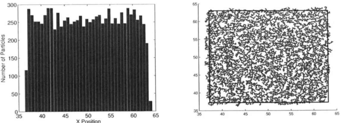
Figure 1-8: Example 10,000-particle packing (from Algorithm 2) with its associated x-position histogram and the boundary selected by the method.

and second, the linear system must be updated to reflect the known voltages.

For the first packing algorithm, identifying the boundary is a trivial process, since the particle locations are known a priori. For algorithm 1.2, however, the particle positions are not known. A boundary can be located visually quite easily at the end of the simulation process, but performing this step manually would be prohibitively slow. In order to expedite and automate the simulation process, the following method was devised to locate the boundary.

First, histograms of the particle x and y positions were separately created. To find the "left" and "right" boundaries, denoted x- and x+ respectively, the histogram of x positions was thresholded. The value x- is defined as the smallest x value where the histogram reaches 50% of its maximum value. The value x+ is defined as the largest x value that meets the same criterion. The top and bottom boundaries, y+ and y-, are found in the same manner using the histogram of particle y coordinates. The threshold value 50% was determined emperically to locate the same boundary that one would identify visually. An example packing and its associated x-position histogram is shown below in figure 1-8 to demonstrate the efficacy of the method. Once the location of the boundary has been identified, all particles whose centers fall less than one radius away from the lines are marked as being "boundary particles". The expression in (1.6) can be computed easily from the solution of the particle

net-work, so by judiciously choosing (E), the components of Ke can be extracted. In two dimensions, the effective conductivity tensor has three independent components, so three simulations are sufficient to extract all of the components. The K1 com-ponent can be extracted by setting (E) = e_. This corresponds to evaluating the integral for an applied boundary voltage of o = -x. The remaining tensor compo-nents may be similarly extracted by applying specific potential fields at the boundary and evaluating the summation given in (1.6).

1.6

Tests

The previously described packing algorithms and solution procedures for the cur-rent/potential have been implemented in Matlab. Algorithm 1.1 was used to create 50,000 separate 400-particle packings. In all of these packings, the F11 and F22

compo-nents of the affine transformation F equalled 1.0. The F12 component that controlled

the shearing of the packing ranged between 0 and 0.5 in increments of 0.01. Any par-ticles that were sheared out of the original bounding rectangle were reflected to the other side of the box to return the packing to a rectangular geometry. We find pack-ing fractions in the range 0

C

[0.65,0.80]. Algorithm 1.2 was used to create 10,000 separate 5,000-particle packings. In the B matrix, the B11 component remained 1.0,

and the B22 component was varied in [1.0, 1.9] in increments of 0.1 to influence the

level of anisotropy of the resulting packings. The approximate range of packing frac-tions we find is 0 E [0.45, 0.'70]. After applying the previously described procedure to each packing to obtain the effective conductivity tensor and average fabric tensor for each packing, the data were analyzed to determine how well the results agree with the model's predictions for the isotropic magnitude, the deviatoric magnitude, and the direction of conductivity. If the model is successful, then for any choice of A, the model should match the ensemble average conductivity of all packings having that fabric A. Below, for ease of demonstration, we bin the data based on scalar invari-ants of A, and show either the ensemble average of the conductivity data at different

choices of those scalars, or simply show scatter-plot comparisons against the full set of tests when it is more illustrative to do so. These tests are described next, and thereafter we shall proceed to show how well the lattice model performs compared to the existing model, equation (1.18).

The isotropic behavior of the conductivity can be investigated by taking the trace of both sides of (1.16). The average coordination number is the most natural inde-pendent variable when examining the isotropic behavior, so in addition to taking the trace of both sides of (1.16), both sides were multiplied by det A in order to make

the right-hand side a single-valued function of trA. This results in (1.21).

R, trK det A = (trA - 2) trA (1.21)

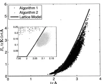
The results of the simulations are scatter-plotted together with the analytical curve given by (1.21) in figure 1-9. It was found that the analytical solution is usually an upper bound on the measured conductivity. This can be explained by the fact that the analytical model was derived from an idealized system where the chains span a unit cell in a straight line. Since the total resistance of a chain is proportional to the number of contacts in the chain, it follows that the shortest chain between any two points is the lowest resistance path, and therefore most conductive. Since the model was derived from a straight-chain idealization, it implies an upper bound on the conductivity. This logic is less valid in low-coordinated systems, which have many disconnected groupings of one or two particles; low-coordinated systems rarely if ever occur from Algorithm 2 or in actual carbon black suspension networks. In this case, the trace of the system's fabric can be less than 2 but percolating chains may still

exist to produce small but non-zero conductivity. This effect is evident in the figure in the data of Algorithm 1.

Next, we determine the extent the analytical lattice model predicts the anisotropy of the conductivity. To remove the influence of the isotropic behavior, we take the

5 4 -D3 2 1 0 1 2 3 4 trA

Figure 1-9: Predicted relationship between the (modified) trace and the fabric trace, compared to numerical results of 50,000 by Algorithm 1 and 10,000 generated under Algorithm 2. Inset

vicinity of trA = 2.

of the conductivity packings generated is a zoom-in of the

deviator of both sides of (1.16). In this case, the most natural independent variable is the magnitude of the fabric deviator, so the resulting equation was manipulated to be a single-valued function of this quantity. After manipulation, (1.16) can be written as (1.22).

(1.22) RKO: Ao det A

lAol (trA - 2 I

where a subscript 0 denotes the deviator of the tensor, and the term A is commonly referred to as the direction or sign of the tensor A0. The left hand side was plotted against |Aol by binning all the test data by lAol and ensemble averaging in each bin. It can be seen in figure 1-10 that, although there is a large amount of noise in the

measurements, the model captures the average behavior very closely.

The final prediction that must be examined is the notion of codirectionality. The analytical model in (1.16) predicts that the fabric and conductivity tensors have the same eigenvectors. To examine this, the angle difference between the fabric and con-ductivity deviators was calculated, which is equivalent to the (signed) angle between the eigenvectors corresponding to the largest eigenvalues of the two tensors, denoted eK and eA. The deviators were chosen because, in 2D, the eigenvector

correspond-34 Algorithm 1 Algorithm 2 - Lattice Model 0.2s 0.15 0.1.-0.05 1.95 2 2.05 2.1 2.15

C4 1. -0. -1' 0 0.1 0.2 0.3 0.4 0.5 0.6 |Aoj

Figure 1-10: Predicted relationship between effective magnitude of the anisotropy of the conductivity and the invariants of the fabric. Error bars show one standard deviation.

ing to the positive eigenvalue can be unambiguously chosen. The probability density function of the angle difference as a function of AO is plotted in figure 1-11. It can be seen that this distribution is symmetrically centered around zero, indicating that the fabric and conductivity are strongly codirectional.

Finally, we also compared the lattice model, (1.16), to the existing model by Jagota & Hui[26l shown in (1.18). For the same 60,000 packings generated using both packing algorithms, we computed the relative error of the prediction of the trace and the determinant of the conductivity using each model and plotted the results in figures 1-12 and 1-13. In every case, we found that the new lattice model predictions were closer to the true values from the numerical experiments than the previous model by Jagota & Hui. On the other hand, the Jagota & Hui model maintains a strong upper bound on both invariants of the conductivity tensor, whereas the lattice model is not strictly an upper bound, as previously discussed. In addition, since the isotropic part of the Jagota & Hui model is identical to the Hashin-Shtrikman upper bound on conductivity, Figure 1-12 also indicates that the Lattice Model is falling within this bound. To be more precise, the lattice model prediction for the isotropic part of

v Algorithm 1

' Algorithm 2 - Lattice Model

1.4 eK 1.2 -AO 1 e 0.80.6 - 0.4- 0.2-01 -2 -1 0 1 2 AO (radians)

Figure 1-11: PDF of angle differences are distributed around zero, indicating codirec-tionality of the fabric and conductivity tensors, as predicted by the analytical model, i.e. (1.16).

conductivity is always less than the Hashin-Shtrikman upper bound computed for a given packing.

1.7

Discussion and Conclusions

In this paper we have derived and tested a new model relating the structure of a packing of particles to its tensorial electrical conductivity. The assumptions implicit in the model are that the suspending medium is a perfect insulator and that electri-cal resistance arises only at particle contacts. The structural measurement used was the fabric tensor, and the model arises from a straightforward analysis of a represen-tative problem involving a lattice structure. The resulting model takes a nonlinear functional form, and was tested multiple ways against numerical simulations of many

thousands of random particle packings. The agreement in its predictions of the

var-ious scalar properties and tensorial orientation is significant, especially in light of

0

-Lattice Model

-Lattice Model

Jagota & Hui Jagota & Hui

5

0

-4--D

0.5 1 1.5 2 0 0.05 0. 1 0.15 0.2 0.25

trK trK

Figure 1-12: Plot of the relative error of the trace of conductivity. (Left) Relative error from packings created with Algorithm 1.1. (Right) Relative error from packings created with Algorithm 1.2.

Lattice Model - Lattice Model

50 Jagota Hui u Jagota & Hui

40- 50- 30-1 20-0 " 10 0 0.2 0.4 0.6 0.8 500 0.005 0.01 0.015 detK detK

Figure 1-13: Plot of the relative error of the determinant of conductivity. (Left) Relative error from packings created with Algorithm 1.1. (Right) Relative error from packings created with Algorithm 1.2.

model. In our tests, the lattice model's accuracy was shown to be higher than an existing conductivity model, a model which requires more structural input data than the lattice model. While it is definitely possible to write a more accurate model by including dependences on more structural variables - some of our data spread is due to the finite nature of the datasets, but some is surely due to modeling error -the current simplicity of -the lattice model is an advantage for its usage in engineer-ing applications involvengineer-ing flowengineer-ing suspension networks. Modelengineer-ing frameworks for the evolution of anisotropy tensors in flowing media have been developed over the last decades[20, 17, 351; keeping our model in terms of fabric, then, suggests a path to the simulation of simultaneous flow and current transfer fields in nontrivial systems by coupling a fabric evolution rule and a rheology with our conductivity model. Such a

capability would be key in the targeted application of modeling flow battery systems, which rely on a flowing conductive suspension that closely resembles the idealized system that we considered. A second direction for future work would be to apply the same idea of simultaneous flow and anisotropy modeling to other transport phenom-ena. For example, incompressible flow through a deforming granular media would have a similar mathematical formulation, albeit with reversed spatial assumptions since the impermeable grains play the role of the insulating medium here. The fabric tensor could be used as a surrogate to describe the structure of the pore space, which would relate to anisotropic permeability.

1.8

Acknowledgements

The authors acknowledge support from the Joint Center for Energy Storage Research (JCESR), an Energy Innovation Hub funded by the U.S. Department of Energy, Office of Science, Basic Energy Science (BES). The authors declare that there are no conflicts of interest.

Chapter 2

Suspension Microstructure Evolution

2.1

Introduction

Material anisotropy has been an active area of interest in many fields for decades. It plays a critical role in such fields as biomechanics

18,

131, plasticity [171, granular materials [3, 12, 31, 33, 35, 37, 41], liquid crystals [401, and more. Some materials, such as elastic composites, have fixed anisotropy that does not evolve over time. However, other materials may develop anisotropy due to deformation, as in the well-known kinematic hardening plasticity theory of Armstrong and Frederick

117].

Still others may develop anisotropy due to an externally-applied field, such as an electric field. This behavior is typical of liquid crystals [40J.

Of particular interest in this study is the flow-induced anisotropy in colloidal sus-pensions. Suspensions of carbon black, an electrically-conductive form of carbon that has recently found application in a new class of batteries called "flow batteries"

114,

461. The carbon black creates an electrically conductive network inside the flow-ing electrolytes of the battery, allowflow-ing for much higher reaction rates and overall system efficiency. However, it has been experimentally demonstrated that the net-works in these carbon suspensions are highly sensitive to shearing

11,

2, 7, 38]. In

these studies, the conductivity of the carbon network drops precipitously with shear and recovers dynamically when brought to rest. This has serious implications for battery performance if the evolution of network structure and conductivity are not properly handled during design. Recent studies [39] on optimizing the efficiency of a flow battery have neglected the effect of a shear-induced drop in suspension conduc-tivity. In addition to the drop in conductivity, it has been shown that suspensions become anisotropic during shearing flow, which can lead to anisotropic conductiv-ity [25, 32, 45]. In this study, we will develop a frame-indifferent constitutive law for the evolution of a tensor-valued measure of network anisotropy and combine this model with previous conductivity modeling work to make quantitative predictions of conductivity evolution during flow.

2.1.1

Necessary Background

To describe the structure of the particle network in suspension, we use a tensor-valued measure called the "fabric tensor." It was originally devised to describe the contact network inside a dense granular material [31, 33, 37]. The fabric tensor is a second-order tensor that can be defined at the particle level with the relation

Neontacts

AP =n(' o n(' (2.1)

where 0 denotes the dyadic product of contact unit normal vectors ni. This is illustrated in figure 2-1. Often, however, it is more illustrative to examine the average fabric of a group of particles rather than the particle-level information. The averaging can be done in

Nparticles

A = N

3

(AP), (2.2)

This definition of the fabric tensor yields a number of useful properties. First, the trace of A' is equal to the coordination number of contacts on a particle. Con-sequently, trA represents the average coordination number, usually denoted Z, of

Figure 2-1: Schematic of particles in contact showing contact vectors n(').

a group of particles. Second, this definition of A results in a symmetric, positive semi-definite tensor. This means that the eigenvalues of A are non-negative, and the eigenvectors are orthogonal. This is appealing, because these properties are shared by the conductivity tensor K.

In previous work

[34],

we modeled the conductivity tensor of a network as a function of the average fabric tensor A. To do this, we assumed that a particle network could be represented by a regular lattice of particles with the same average fabric tensor. It is simple, then, to compute the effective conductivity and average fabric tensors of the regular lattice in terms of the lattice dimensions. We then inverted the fabric-lattice relationship to obtain the conductivity in terms of the fabric tensor directly. See Olsen and Kamrin 2015 1341 for a more detailed explanation. We found that

K = k (trA 2)2 A. (2.3)

det A

2.2

Evolution Law

Faced with the aforementioned experimental evidence that the contact network of a suspension changes due to flow, we set out to develop a continuum model that can accurately characterize the evolution of the network under arbitrary flow fields. Al-though the fundamental quantity that we model, the particle network, is composed of discrete units, we make a continuum approximation. In the continuum approxi-mation, quantities at a point really represent averages of quantities, such as velocity or fabric, that are defined discretely at much smaller length scales. This is a valid

approximation since typical applications of these particle networks are several orders of magnitude larger than the constituents of the networks. As a concrete example, the particles of carbon black are - 100nm, while the features in a flow battery are ~ 1mm. Therefore, we can use the language of modern continuum mechanics to describe the evolution of the fabric tensor 1191. We define the velocity gradient L, the stretching (strain-rate) tensor D, and the spin tensor W below.

L = (2.4)

D sym(L) = (L + LT) (2.5)

1

W = skw(L) = (L - LT) (2.6)

We postulate a fabric evolution law of the form A f(A, L), where A denotes

the material time derivative of A. In order for an evolution law such as this to be

indifferent under a change in an observer's frame of reference, the evolution law must be of the form

i=WA

- AW + f(A, D) (2.7)

where where A denotes the material time derivative of A and f is an isotropic function

of the fabric tensor and the stretching tensor [201. Using the Caley-Hamilton theorem,

Rivlin derived a representation theorem for 3 x 3 symmetric tensors as a function of

two other 3 x 3 symmetric tensors 1361. Using this, we can write the evolution law as

+ AW - WA cC11+ c 2A + c3D + 4A2 + c5 D2 + c(AD + DA)

+c7(A2D + DA2) + c8(AD2 + D2A) + c9(A2D2 + D2A2) (2.8)

simul-taneous invariants of A and D .

trA, trA2, trA3 trD, trD2

, trD3 _(2.9)

trAD, trA2_{D, trAD}2_{, trA}2_D2

The left-hand side of (2.8) is known as the co-rotational time derivative of the tensor field A. In the solid mechanics literature, it is frequently referred to as the Jaumann rate, and is given the symbol A. In general, the left-hand side can be any objective time derivative of the tensor field, and it can be shown that they are all specializations of the Lie derivative

[291.

We chose to use the co-rotational time derivative so that we, as modelers, retain full control over the evolution of A in its principal frame. Other objective rates, such as the contravariant or covariant time derivatives, contain terms that would contribute in this way 1191.

2.2.1

Specialization of Constitutive Equation

The fully general form of the evolution law, shown in (2.8), has a large number of scalar functions that must be specified. In order to reduce the risk of overfitting our model; we chose to set ci - 0 for i > 4. This leaves us with all of the tensorially

linear terms and their associated coefficients.

A= c11 + c2A+ c3D (2.10)

The task of modeling, therefore, is reduced to choosing the coefficients ci, c2, and c3

in a physically meaningful way.

Physical Intuition and Constraints

By examining the effect of each term on the evolution of the fabric, some intuition and observation can be applied to reduce the space of possible coefficients ci. There

are some key observations that must be qualitatively matched before any more de-tailed modeling work can proceed. First, at steady state, the fabric will be positive, isotropic, and unchanging in the absence of flow. This requires that any anisotropy induced by flow relax away over time. Second, contacts are formed on the compres-sive axis of shearing flow and broken on the extension axis. This was experimentally observed by Hoekstra et al.1251. Lastly, we observe that the electrical conductivity of a suspension decreases with increasing shear rate. However, the conductivity never reaches zero. Since we have derived a model, (2.3), for electrical conductivity in terms of the fabric tensor, we can use this to put further constraints on the evolution law.

We can translate these observations directly into constraints on the coefficients. The condition that the fabric relaxes to an isotropic steady state in the absence of flow

implies the following two constraints.

c1(IA,D) >0 VA,D (2.11)

C2(IA,D) < 0 V A,D (2.12)

If either of these constraints were violated, then the fabric would either decay away to a non-positive isotropic state or diverge. The precise nature of the decay or divergence depends on the functional forms of ci and c2 and will be examined in greater detail

in the following sections where these functions are specified.

The sign of c3 can be identified from the second observation. By examining the pure

shear evolution of A in the principal basis of D, it becomes clear that in order for the observations in Hoekstra[25l and Morris

1321

to be correctly represented, c3 must obey

C3(IA,D) <0 V A, D. (2.13)

A third constraint can be formed from the experimental observation that conductivity never entirely disappears, even at high shear rate[2]. Based on the conductivity model assumption in (2.3), this implies that trA remains above 2 at all times. To find the

conditions on the evolution law coefficients that must be true, we take the trace of (2.10) and solve for the steady-state trace of the fabric trA,,. The flow is assumed to be incompressible, so trD = 0. 0 = 3 c, + C2 trA,8 trA, =- > 2 C2 cl 2 - - ->- VA,D (2.14) c2 3

The final constraint is of mathematical origin. By closely examining the definition of the fabric tensor in (2.1), it quickly becomes evident that no diagonal component of A can have a negative value. A physical interpretation of this property of A is that it is not possible to have a negative number of contacts in any principal direction. Consequently, this condition also prevents any negative diagonal values of conductivity, and in so doing prevents negative dissipation, which would be a violation of the second law of thermodynamics. A constraint can be formed from this by examining the steady-state values of the diagonal components of A in an incompressible, spin-free flow (i.e. W = 0).

O = c11 + c2A+ c3D

1

A = -- _{(c11 + c3D)}

C2

Without loss of generality, we can examine the component Al and set it to be > 0.

1

An = -- (c1 + c3DI) > 0 (2.15)