Construction of a complete set of orthogonal Fourier-Mellin moment invariants for pattern recognition applications

HAL Id: inserm-00420576

https://www.hal.inserm.fr/inserm-00420576

Submitted on 29 Sep 2009

HAL is a multi-disciplinary open access archive for the deposit and dissemination of sci-entific research documents, whether they are pub-lished or not. The documents may come from teaching and research institutions in France or abroad, or from public or private research centers.

L’archive ouverte pluridisciplinaire HAL, est destinée au dépôt et à la diffusion de documents scientifiques de niveau recherche, publiés ou non, émanant des établissements d’enseignement et de recherche français ou étrangers, des laboratoires publics ou privés.

Construction of a complete set of orthogonal

Fourier-Mellin moment invariants for pattern

recognition applications

Hui Zhang, Huazhong Shu, Pascal Haigron, Limin Luo, Baosheng Li

To cite this version:

Hui Zhang, Huazhong Shu, Pascal Haigron, Limin Luo, Baosheng Li. Construction of a complete set of orthogonal Fourier-Mellin moment invariants for pattern recognition applications. Image and Vision Computing, Elsevier, 2010, 28 (1), pp.38-44. �10.1016/j.imavis.2009.04.004�. �inserm-00420576�

Construction of a complete set of orthogonal Fourier-Mellin moment

invariants for pattern recognition applications

H. Zhang1_{, H. Z. Shu}1, 5_{, P. Haigron}2, 3, 5_{, B.S. Li}4_{, L. M. Luo}1, 5

1_{Laboratory of Image Science and Technology, School of Computer Science and Engineering,}

Southeast University, 210096 Nanjing, China

2_{INSERM, U642, 35042 Rennes, France}

3_{Laboratoire Traitement du Signal et de l’Image, Université de Rennes I, 35042 Rennes,}

France

4_{Department of Radiation Oncology, Shandong Cancer Hospital, 250117 Jinan, China} 5_{Centre de Recherche en Information Biomédicale Sino-français (CRIBs)}

Information about the corresponding author

Huazhong Shu, Ph.D

Laboratory of Image Science and Technology

School of Computer Science and Engineering

Southeast University, 210096, Nanjing, China

Tel: 00-86-25-83 79 42 49

Fax: 00-86-25-83 79 26 98

Email: shu.list@seu.edu.cn

Abstract The completeness property of a set of invariant descriptors is of fundamental

importance from the theoretical as well as the practical points of view. In this paper, we

propose a general approach to construct a complete set of orthogonal Fourier-Mellin moment

(OFMM) invariants. By establishing a relationship between the OFMMs of the original image

and those of the image having the same shape but distinct orientation and scale, a complete

set of scale and rotation invariants is derived. The efficiency and the robustness to noise of the

method for recognition tasks are shown by comparing it with some existing methods on

several data sets.

Key Words: Orthogonal Fourier-Mellin moments, Completeness, Similarity invariants,

Moment invariants, Pattern recognition

1. Introduction

Description of objects invariant to geometric transformations such as translation, scale

and rotation is a basic tool in pattern recognition. The performance of pattern recognition

systems depends on the specific feature extraction technique used to represent a pattern. A

popular class of invariant features is based on the moment techniques including geometric

moment, complex moments and orthogonal moments [1-9]. Among them, moments with

orthogonal basis functions can represent the image by a set of mutually independent

descriptors and thus have a minimal amount of information redundancy. As noted by Ghorbel

et al. [10, 11], the most important properties to assess by the image descriptors are: (1)

invariance against some geometrical transformations (translation, rotation, scaling); (2)

In the past decades, the construction of moment invariants and their application to pattern

recognition have been extensively investigated [12-15]. Since the Zernike moments,

pseudo-Zernike moments and orthogonal Fourier-Mellin moments (OFMMs) are all invariant

under image rotation, they have been successfully used in the fields of image analysis and

pattern recognition [16-24]. A comparative study of the Zernike moments and OFMMs in

terms of recognition accuracy has been recently provided by Kan and Srinath [25]. It was

shown that the OFMMs are better suited for character recognition tasks. The major drawback

however, when using the orthogonal moments, is the lack of native scale invariance. To solve

this problem, the normalization process [18] is often used to achieve the scale invariance.

Such a process may lead to inaccuracy since the normalization of the images requires

re-sampling and re-quantifying. In order to improve the accuracy, Chong et al. [26] recently

proposed a method based on the properties of pseudo-Zernike polynomial to derive the scale

invariants of pseudo-Zernike moments. A similar approach was then used to construct both

translation and scale invariants of Legendre moments [27]. The problem of scale and

translation invariants of Tchebichef moments has been investigated by Zhu et al. [28].

Discrete orthogonal moments such as Tchebichef moments yield better performance than the

continuous orthogonal moments, but it is difficult to derive the rotation invariants. It was

shown that the methods developed in [26-28] perform better than the classical approaches

such as the image normalization method and indirect method. However, it seems difficult to

obtain the completeness property by the above mentioned methods since no explicit

formulation is derived for moment invariants.

two objects have the same shape if and only if they have the same set of invariants [29]. A

number of studies have been conducted on completeness. Flusser et al. proposed a complete

set of rotation invariants by normalizing the complex moments [30, 31]. The construction of a

complete set of similarity (translation, scale and rotation) invariant descriptors by means of

some linear combinations of complex moments has been addressed by Ghorbel et al. [10].

In this paper, we propose a new method to construct a complete set of scale and rotation

invariants extracted from OFMMs. We first establish a relationship between the OFMMs of

the original image and those of the transformed image. Based on this relationship, the

complete set of scale and rotation invariants can thus be achieved.

The organization of this paper is as follows. In Section 2, we review the definition of

OFMMs and the approach proposed by Ghorbel et al. for constructing the complex moment

invariants. Section 3 presents the way to derive a complete set of scale and rotation invariants

of OFMMs. The experimental results for evaluating the performance of the proposed

descriptors are provided in Section 4.

2. Orthogonal Fourier-Mellin moments

This section recalls the definition of OFMMs and briefly describes the method reported

in Ref. [10].

2.1 Orthogonal Fourier-Mellin moments

The two-dimensional (2D) OFMM, Z_pqf , of order p with repetition q of an image intensity

function f(r, θ) is defined as [7] = +

∫∫

− π θ

_θ

_θ

π

2 0 1 0 ) , ( ) ( 1 rdrd r f e r Q p Z jq p f pq , |q| ≤ p (1)

∑

, (2) = = p k k k p p r c r Q 0 , ) ( with )! 1 ( ! )! ( )! 1 ( ) 1 ( ,

₋

₊

+

+

−

=

+

k

k

k

p

k

p

c

p k k p . (3)

Since OFMMs are defined in terms of polar coordinates (r, θ) with |r| ≤ 1, the computation

of OFMMS requires a linear transformation of the image coordinates to a suitable domain

inside a unit circle. Here we use the mapping transformation proposed by Chong et al. [26],

which is shown in Fig. 1. Based on this transformation, we have the following discrete

approximation of equation (1):

∑∑

− = − = −

+

=

1 0 1 0 ) , ( ) ( 1N i N j jq ij p f pq

Q

r

e

f

i

j

p

Z

θij

π

, (4)

where the image coordinate transformation to the interior of the unit circle is given by

2 2 1 2 2 1 ) ( ) (ci c c j c r_ij = + + + , _⎟⎟ ⎠ ⎞ ⎜⎜ ⎝ ⎛ + + = − 2 1 2 1 1 tan c i c c j c ij

θ

(5) with

1

2

1

=

₋

N

c

2 1 2 = c .

2.2 A complete set of invariants extracted from complex moments

Ghorbel et al. proposed a complete set of scale and rotation invariants of complex

moments given by [10] ( ) ( 2) ( , ) p q i p q f ( , ) f f f J p q = Γ− + + e− − θ c p q (6)

where

θ

_f

=

arg(

c

_f

(

1

,

0

))

,

Γ

_f

=

c

_f

(

0

,

0

)

, and is the complex moment of an image function f(x, y) defined as

)

,

( q

p

c

_f

∫ ∫

∫ ∫

∞ _{+ + −} ∞ ∞ − ∞ ∞ − = − + = 0 2 0 ) ( 1 _{( , )} ) , ( ) ( ) ( ) , ( π _θ

θ

θ

drd r f e r dxdy y x f iy x iy x q p c q p i q p q p f p, q ≥ 0. (7)

It can be easily verified that the set of invariants is complete since ( ) ( 2) ( , ) p q i p q f ( , ) f f f c p q _{= Γ} + + e − θ J p q _{. (8)}

Note that in [10], the translation invariance was achieved by transforming the origin of

the image to the geometric center before the calculation of the moments.

3. Method

In this section, a general approach is described to derive a complete set of OFMM

invariants. We use here the same method to achieve the translation invariance as described in

[10]. That is, the origin of the coordinate system is taken at the center of mass of the object to

achieve the translation invariance. This center of mass, (xc, yc), can be computed from the

first geometric moments of the object as follows.

10 01 00 00

,

c c

m

m

x

y

m

m

=

=

, (9) where mpq are the (p+q)th order geometric moments defined by

p q ( , ) . (10)

pq

m ∞ ∞ x y f x y dxdy

−∞ −∞

=

_{∫ ∫}

Let and be two vectors,

where the superscript T indicates the transposition, we have

T m m

r

Q

r

Q

r

Q

r

U

(

)

=

(

₀

(

),

₁

(

),

,

(

))

m T m

r

r

r

r

M

(

)

₌

(

0

,

1

,

,

)

)

(

)

(

r

C

M

r

U

_m

=

_{m m} , (11) where Cm = (ci, j), with 0 ≤ j ≤ i ≤ m, is a (m+1)×(m+1) lower triangular matrix whose element

ci, j is given by Eq. (3).

Since all the diagonal elements of Cm,

)! 1 ( ! )! 1 2 ( , ₊ + = l l l

c_ll , are not zero, the matrix Cm is

non-singular, thus

)

(

)

(

)

(

)

(

_r

_C

1

_U

_r

_D

_U

_r

M

_m

=

_m − _m

=

_{m m , (12)}

where Dm = (di, j), with 0 ≤ j ≤ i ≤ m, is the inverse matrix of Cm. It is also a (m+1)×(m+1)

lower triangular matrix. The computation of the elements of Dm is given in the following

Proposition.

Proposition 1. For the lower triangular matrix Cm whose elements ci, j are defined by Eq. (3),

the elements of the inverse matrix Dm are given as follows

, (2 2) !( 1)! ( )!( 2) i j j i i d i j i j + + = − + + !. (13)

The proof of Proposition 1 is given in Appendix.

Let f and g be two images display the same pattern but with distinct orientation (β) and

scale (λ), i.e., g(r, θ) = f(r/λ, θ–β). The OFMM of the image intensity function g(r, θ) is

defined as 2 1 0 0 2 1 2 0 0

1

( )

( , )

1

( )

( , )

,

g jq pq p jq jq p

p

Z

Q r e

g r

rdrd

p

e

Q

r e

f r

r

π θ π β θ

θ

θ

π

drd

λ

λ

θ

π

− − −

+

=

+

=

∫ ∫

∫ ∫

θ

(14) Letting and

M

it

can be seen from Eq. (11) that

0 1

( ) ( ( ), ( ), ,

( ))

T m m

U

λ

r

=

Q

λ

r Q

λ

r

Q

λ

r

_{( ) (1,( ) , ,( ) )}

1 m T m

λ

r

=

λ

r

λ

r

, ( ) ( ) m m m U

λ

r =C M

λ

r . (15) On the other hand,

1 1 1 ( ) (1, , , )(1, , , ) (1, , , ) ( ). m m m m m T M r diag r r diag M r

λ

λ

λ

λ

λ

= = (16)

Substituting Eqs. (16) and (12) into Eq. (15), we obtain

1

( )

(1, , ,

m

)

( )

m m m m

U

λ

r

=

C diag

λ

λ

D U r

. (17) By expanding Eq. (17), we have

, , 0

( )

( )

p p l p k k l k

Q

λ

r

Q r

λ

c d

= =

=

∑

∑

_{p l l k}. (18) With the help of Eq. (18), Eq. (14) can be rewritten as

2 1 2 0 0 2 1 2 , , 0 0 0 2 1 2 , , _{0 0} 0 2 ,

1

( )

( , )

1

( )

( , )

1

1

( )

( , )

1

1

1

g jq jq pq p p p jq l jq k p l l k k l k p p jq l jq p l l k k k l k jq l p l l

p

Z

e

Q

r e

f r

rdrd

p

e

Q r

c d

e

f r

rdrd

p

k

e

c d

Q r e

f r

rdrd

k

p

e

c d

k

π β θ π β θ π β θ β

λ

λ

θ

θ

π

λ

λ

π

θ

θ

λ

θ

θ

π

λ

− − − − = = − + − = = − +

+

=

⎛

⎞

+

=

_⎜

_⎟

⎝

⎠

+

+

=

×

+

+

=

+

∫ ∫

∑

∑

∫ ∫

∑

∑

_{∫ ∫}

, 0

.

p p f k kq k l k

Z

= =

⎛

⎞

⎜

⎟

⎝

⎠

∑

∑

(19)

The above equation shows that the 2D scaled and rotated OFMMs, , can be

expressed as a linear combination of the original OFMMs with 0 ≤ k ≤ p. Based on this

relationship, we can construct a complete set of both rotation and scale invariants which

is described in the following theorem.

g pq Z f I f kq Z pq

Theorem 1. For a given integer q and any positive integer p, let

( 2) . , 0 1 1 f p p jq f l pq f p l l k kq k l k p f I e c k θ − − + = = ⎛ ⎞ + = _⎜ Γ + ⎝ ⎠

∑

∑

d _⎟Z , (20) with arg( ₁₁f) and

f = Z

θ

f

f = Z00

Γ . Then, is invariant to both image rotation and scaling.

f pq

I

The proof of Theorem 1 is given in Appendix.

Eq. (20) can be expressed in matrix form as

(

)

(

)

0 0 1 _{1, 2, , 1} 2_, 3_{, ,} ( 2) _{1, , ,}1 1 1 _. 2 1 f f f q q f f jq q p q p f f f p f f pq pq I Z I Z

e diag p C diag D diag

p I Z θ − − − − + ⎛ ⎞ ⎛ ⎞ ⎜ ⎟ ⎜ ⎟ ⎛ ⎞ ⎜ ⎟_{= + Γ Γ Γ ⎜ ⎟}⎜ ⎟ ⎜ ⎟ _{⎝ + ⎠}⎜ ⎟ ⎜ ⎟ ⎜ ⎟ ⎜ ⎟ ⎜ ⎟ ⎝ ⎠ ⎝ ⎠ (21)

(

)

(

)

0 0 1 _{1,2, , 1} 2_, 3_{, ,} ( 2) _{1, , ,}1 1 1 2 1 f f f q q f f jq q p q p f f f p f f pq pq Z I Z I

e diag p C diag D diag

p Z I θ + ⎛ ⎞ ⎛ ⎜ ⎟ ⎜ ⎛ ⎞ ⎜ ⎟_{= + Γ Γ Γ} ⎜ ⎜ ⎟ ⎜ ⎟ _{⎝ + ⎠}⎜ ⎜ ⎟ ⎜ ⎜ ⎟ ⎜ ⎝ ⎠ ⎝ ⎞ ⎟ ⎟ ⎟ ⎟⎟ ⎠ . (22) Thus, we have

∑

∑

= = + ⎟⎟ ⎠ ⎞ ⎜⎜ ⎝ ⎛ _Γ + + = p k f kq p k l pl lk l f jq f pq _k c d I p e Z f 0 , , ) 2 ( 1 1 θ (23)

The above equation shows that the set of invariants is complete.

4. Experimental results

This section is intended to test the performance of the complete family of similarity

invariants introduced in this paper using a set of gray-level images.

In the first experiment, a toy cat image whose size is 128×128 pixels is chosen from the

well-known Columbia database [32] (Fig. 2). The proposed invariant descriptors are

compared to the complete set of complex moment invariants (CMI) reported in [10]. To make

the comparison possible between all families of invariants, we rearrange the complex moment

invariants following the scheme presented in Ref. [10] through the path (1, 0)→1, (0, 1)→2,

(2, 0)→3, (1, 1)→4, (0, 2)→5, (3, 0)→6, and so on. Let M be the maximum order of complex

moment invariant, and let , where

J ( ) ( (1, 0), (0,1), , ( , 0), , (0, )) f C f f f f C M = J J … J M … J M

( )

f C

C M

1), , ( , 0), , ( ,… I M_f … I M M_f ))

)

M

f(p, q) are defined by Eq. (6). The dimension of is (M+1)(M+2)/2–1. For

comparison purpose, we also define the vector

for OFMM invariants (OFMMI).

The dimension of is also (M+1)(M+2)/2–1. In this experiment M = 4 is chosen,

that is, 14 invariants from first to fourth order are used.

( ) ( (1, 0), (1, f FM f f C M = I I

(

f FM

C

the original image f(x, y) and the transformed image g(x, y) as || ( ) ( ) || ( , ) || ( ) || f g M f C M C M E f g C M − = , (24) where ||.|| is the Euclidean norm.

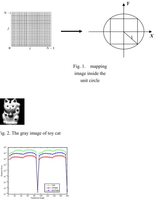
To test the invariance against rotation, we have rotated the original image from 0° to

180° with interval 5°. Because the magnitude of the OFMM is invariant to image rotation, we

also take it as rotation invariant feature of the underlying image function. Fig. 3 compares the

relative errors between the proposed method, CMI and the magnitude of the OFMMs

(MOFMM) using Eq. (24). It can be seen from this figure that the OFMMI outperforms the

other two methods, whatever the rotational angle. We then evaluate the invariance of the

proposed descriptors with regard to image scaling. The toy cat image is scaled by a factor

varying from 0.1 to 2 with interval 0.05. Fig. 4 shows the relative errors of the OFMMI, CMI,

the normalization method presented in [18] and the scale invariants of OFMM derived by the

method presented in Ref. [26] (we call it Chong’s method for abbreviation). Plots show that,

in most cases, the relative errors of OFMMI and Chong’s method are lower than those of the

CMI and normalization method. To test the robustness to noise, we have respectively added a

white Gaussian noise (with mean μ = 0 and different variances) and the salt-and-pepper noise

(with different noise densities). Results are respectively depicted in Fig. 5 and Fig. 6. It can

be seen that, if the relative error increases with the noise level, the proposed descriptors are

more robust to noise than the CMI and Chong’s method.

We also compare the computational speed of the OFMMI with that of the CMI and other

methods. The computation time required in the above experiments for different methods is

the program was implemented in MATLAB 6.5 on a PC P4 2.4 GHZ, 512M RAM, and the

computation of the OFMMIs was performed from Eq. (21). It can be seen that the OFMMI is

faster than most of the other methods, this is due to the following two facts: (1) the fast

algorithm presented in Ref. [23] was applied; (2) the matrix representation is very useful and

efficient for software packages such as MATLAB.

We now test the classification accuracy of the proposed method, CMI and Chong’s method

with scaled and rotated image in both noise-free and noisy conditions. For the recognition

task, we use the following feature vector

V = [I1, I2, I3, I4, I5, I6, I7], (25)

where Ij, j = 1, 2, …, 7, denote the second and third order of CMI or OFMM invariants. The

objective of a classifier is to identify the class of the unknown input object. During the

classification, features of the unknown object are compared to a set of testing samples. The

Euclidean distance is used as the classification measure and is defined by

∑

= − = 7 1 2 ) ( _{) ( )} , ( j t j s j k t s V I I V d , (26)

where is the 7-dimensional feature vector of unknown sample, and is the testing

vector of class k. The classification accuracy is defined as

s

V (k)

t

V

100%

Number of correctly classified images The total number of images used in the test

η

= ×

. (27)

Fig. 7 shows a set of object images selected from the Coil-100 image database of

Columbia University [32]. The reason for choosing such a set is that the objects (three toy

cars, three blocks, ANACIN and TYLENOL packs) can be easily misclassified due to their

factor λ ∈{0.5, 0.75, 1, 1.5, 2} and rotation angle β∈{30°, 60°, ……, 330°, 360°}, forming a

set of 480 images. This is followed by adding the salt-and-pepper noise with different noise

densities. The feature vector based on our method is used to classify these images and its

recognition accuracy is compared to CMI as well as Chong’s method. Table 2 shows the

classification results using the full set of features. One can observe from this table that the

high recognition rates are obtained in noise-free case. The recognition accuracy decreases

with increasing noise level. However, the proposed method performs better than the CMI and

Chong’s method in terms of the recognition accuracy for noisy images.

In the last experiment, a set of alphanumeric characters whose size are 50×50 pixels

shown in Fig. 8 is used for recognition task. The images are transformed by scaling and

rotating the original set with scale factor λ ∈{0.5, 1, 2} and rotation angle β∈{15°, 30°, ……,

345°, 360°}, forming a set of 576 images. The salt-and-pepper noise with different noise

densities has been added. Some examples of the test images are illustrated in Fig. 9. The

classification results are listed in Table 3. It can be seen that our method is more robust than

other methods for noisy images.

5. Conclusion

In this paper, we have presented a novel method to derive a complete set of OFMM

invariants. Since the proposed method extracts the invariant feature from the orthogonal

Fourier-Mellin moments of the original image, no image normalization process is required.

Experimental results show that our method has a better classification accuracy and is more

Acknowledgement: This work was supported by Program for Changjiang Scholars and

Innovative Research Team in University and by the National Natural Science Foundation of

References

1. M.K. Hu, Visual pattern recognition by moment invariants, IRE Transactions on

Information Theory, 8 (1962) 179-187.

2. J. Flusser, T. Suk, Pattern recognition by affine moment invariants, Pattern Recognition,

26 (1993) 167-174.

3. M. Teague, Image analysis via the general theory of moments, Journal Optical Society

America, 70 (1980) 920-930.

4. C.H. Teh, R.T. Chin, On image analysis by the method of moments, IEEE Transactions

on Pattern Analysis and Machine Intelligence, 10 (1988) 496-513.

5. S.S. Reddi, Radial and angular moment invariants for image identification, IEEE

Transactions on Pattern Analysis and Machine Intelligence, 3 (1981) 240-242.

6. Y.S. Abu-Mostafa, D. Psaltis, Recognitive aspects of moment invariants, IEEE Transactions

on Pattern Analysis and Machine Intelligence, 6 (1984) 698-706.

7. Y.L. Sheng, L.X.Shen, Orthogonal Fourier-Mellin moments for invariant pattern

recognition. Journal Optical Society America, 11 (1994) 1748-1757.

8. T. Xia, H.Q. Zhu, H.Z. Shu, P. Haigron, L.M. Luo, Image description with generalized

pseudo-Zernike moments, Journal Optical Society America, 24 (2007) 50-59.

9. S. Rodtook, S.S. Makhanov, Numerical experiments on the accuracy of rotation moments

invariants, Image and Vision Computing, 23 (2005) 577-586.

10. F. Ghorbel, S. Derrode, R. Mezhoud, T. Bannour, S. Dhahbi, Image reconstruction from a

Recognition Letters, 27 (2006) 1361-1369.

11. S. Derrode, F. Ghorbel, Robust and efficient Fourier-Mellin transform approximations for

invariant grey-level image description and reconstruction, Computer Vision and Image

Understanding, 83 (2001) 57-78.

12. Y. Li, Reforming the theory of invariant moments for pattern recognition, Pattern

Recognition, 25 (1992) 723-730.

13. J. Liu, T.X. Zhang, Fast algorithm for generation of moment invariants, Pattern

Recognition, 37 (2004) 1745-1756.

14. D. Xu, H. Li, Geometric moment invariants, Pattern Recognition, 41 (2008) 240-249.

15. Y. C. Chim, A. A. Kassim, Y. Ibrahim, Character recognition using statistical moments,

Image and Vision Computing, 17 (1999) 299-307.

16. Z.J. Miao, Zernike moment-based image shape analysis and its application, Pattern

Recognition Letters, 21 (2000) 169-177.

17. W.Y. Kim and Y.S. Kim, A region-based shape descriptor using Zernike moments, Signal

Processing: Image Communication, 16 (2000) 95-102.

18. A. Kontanzard, Y.H. Hong, Invariant image recognition by Zernike moments, IEEE

Transactions on Pattern Analysis and Machine Intelligence, 12 (1990) 489-497.

19. R.R. Bailey and M.D. Srinath, Orthogonal moment features for use with parametric and

non-parametric classifiers, IEEE Transactions on Pattern Analysis and Machine

Intelligence, 18 (1996) 389-399.

20. A. Broumandnia, J. Shanbehzadeh, Fast Zernike wavelet moments for Farsi character

21. T.J. Bin, A. Lei, J.W. Cui, W.J. Kang, D.D. Liu, Subpixel edge location based on

orthogonal Fourier–Mellin moments, Image and Vision Computing, 26 (2008) 563-569.

22. B. Ye, Improvement of orthogonal Fourier-Mellin moments, Proceedings of SPIE - The

International Society for Optical Engineering 5985 PART II, (2005) 598531.

23. G.A. Papakostas, Y.S. Boutalis, D.A. Karras, B.G. Mertzios, Fast numerically stable

computation of orthogonal Fourier-Mellin moments, IET Computer Vision 1 (2007)

11-16.

24. B. Fu, J.Z. Zhou, J.Q. Wen, An efficient algorithm for fast computation of orthogonal

Fourier-Mellin moments, Proceedings of SPIE - The International Society for Optical

Engineering 5985 PART II, (2005) 59853A.

25. C. Kan, M.D. Srinath, Invariant character recognition with Zernike and orthogonal

Fourier-Mellin moments, Pattern Recognition, 35 (2002) 143-154.

26. C.W. Chong, P. Raveendran, R. Mukundan, The scale invariants of pseudo-Zernike

moments, Pattern Analysis and Applications 6 (2003) 176-184.

27. C.W. Chong, P. Raveendran, R. Mukundan, Translation and scale invariants of Legendre

moments, Pattern Recognition, 37 (2004) 119-129.

28. H.Q. Zhu, H.Z. Shu, T. Xia, L.M. Luo, J.L. Coatrieux, Translation and scale invariants of

Tchebichef moments, Pattern Recognition, 40 (2007) 2530-2542.

29. T.R. Crimmins, A complete set of Fourier descriptors for two dimensional shape, IEEE

Transactions on Systems, Man and Cybernetics, 121 (1982) 848– 855.

30. J. Flusser, On the independence of rotation moment invariants. Pattern Recognition, 33

31. J. Flusser, On the inverse problem of rotation moment invariants. Pattern Recognition, 35

(2002) 3015–3017.

32. http://www1.cs.columbia.edu/CAVE/software/softlib/coil-20.php

33. M. Petkovsek, H. S. Wilf, and D. Zeilberger, A=B, AK Peters (1996). (available on line at

Appendix

Proof of Proposition 1. To prove the proposition, we need to demonstrate the following

relation l k k l s l s s k

d

c

_{, ,}

=

δ

_,

∑

= . (A1) For k = l, we have 1 )! 2 2 ( )! 1 ( ! ) 2 2 ( )! 1 ( ! )! 1 2 ( , , ₊ = + + × + + = k k k k k k k d c_{kk kk} . (A2) For l < k, we have , ,

(

1

)!(2

2)

( 1)

(

)!(

)!(

2)!

( 1) (2

2)

( , , ),

k k k s k s s l s l s l k k s l

k

s

l

c d

k s s l

s l

l

F k l s

+ = = =

+ +

+

=

−

−

−

+ +

= −

+

∑

∑

∑

(A3) where )! 2 ( )! ( )! ( )! 1 ( ) 1 ( ) , , ( + + − − + + − = l s l s s k s k s l k F s . (A4) Letting 1 ( 1) ( 1 )! ( 1 )( ) ( , , ) ( 1 )!( )!( 1)! ( )( 2 s _{k s k s s} G k l s k s s l s l k l k l + − + + + − − = + − − + + − + + ) l

=

, (A5)

it can then be easily verified that

)

,

,

(

)

1

,

,

(

)

,

,

(

k

l

s

G

k

l

s

G

k

l

s

F

=

+

−

. (A6) Thus

( , , )

[ ( , ,

1)

( , , )]

( , ,

1)

( , , ) 0,

k k s l s l

F k l s

G k l s

G k l s

G k l k

G k l l

= =

=

+ −

=

+ −

∑

∑

_(A7)

0

, ,

=

∑

= k l s l s s k

d

c

for l < k.

The proof is now complete.

Note that the proof of Proposition 1 was inspired by a technique proposed by Petkovsek et al

[33].

Proof of Theorem 1. Eq. (20) can be rewritten in matrix form as

0 1 0 1 2/2 3/2 ( 2)/2 00 00 00 (1,2, , 1) 1 1 ( , , , ) (1, , , ) 2 1 g g q g jq q p g pq g q g q g g g p p g pq I I e diag p C I Z Z diag Z Z Z D diag p Z θ − − − − + ⎛ ⎞ ⎜ ⎟ ⎜ _{⎟ = +} ⎜ ⎟ ⎜ ⎟ ⎜ ⎟ ⎝ ⎠ ⎛ ⎞ ⎜ ⎟ ⎜ ⎟ × _{⎜ ⎟} + ⎜ ⎟ ⎜ ⎟ ⎝ ⎠ (A8)

Using the same representation, Eq. (19) can be expressed by

0 1 2 3 2 0 1 (1, 2, , 1) ( , , , ) 1 1 (1, , , ) 2 1 g q g q jq p p p g pq f q f q f pq Z Z e diag p C diag D Z Z Z diag p Z β _{λ λ λ} − + ⎛ ⎞ ⎜ ⎟ ⎜ _{⎟ = +} ⎜ ⎟ ⎜ ⎟ ⎜ ⎟ ⎝ ⎠ ⎛ ⎞ ⎜ ⎟ ⎜ ⎟ × _{⎜ ⎟} + ⎜ ⎟ ⎜ ⎟ ⎝ ⎠ (A9) In particular, we have 2 00 00 1,1

,

arg(

)

.

g f g g f

Z

Z

Z

λ

θ

θ

β

=

=

=

−

(A10)

(

)

(

)

(

)

(

)

, 2, 2/ 2 3/ 2 ( 2) / 2 00 00 00 2 , 0 1 2 3 ( 2) 1, 2, , 1 , , , 1 1 , , , 1, , , 2 1 1, 2, , 1 ( f f g q q g jq q q jq f f f p p g q m q g q g q p p g pq jq jq p I I e e diag p C diag Z Z Z I Z Z diag D diag p Z e e diag p C diag θ β θ β

λ λ

λ

− + − − − + + − − − + − ⎛ ⎞ ⎜ ⎟ ⎜ _{⎟ = +} ⎜ ⎟ ⎜ ⎟ ⎜ ⎟ ⎝ ⎠ ⎛ ⎞ ⎜ ⎟ ⎛ _{⎞⎜ ⎟} × _{⎜ ⎟⎜ ⎟} + ⎝ _{⎠⎜ ⎟} ⎜ ⎟ ⎝ ⎠ = +

(

)

(

)

(

)

2/ 2 3/ 2 ( 2) / 2 00 00 00 2 3 ( 2) 0 1 2 3 2 , , , ) 1 1 , , , 1, , , 2 1 1 1 1, 2, , 1 , , , 1, , , 2 1 f f f p p p f q f q jq p p p f pq Z Z Z diag D diag p Z Z

e diag p C diag D diag

p Z β

λ λ

λ

λ λ

λ

− − − + − − − + − + ⎛ ⎞ × _{⎜ ⎟} + ⎝ ⎠ ⎛ ⎞ ⎜ ⎟ ⎛ _{⎞⎜ ⎟} × + _{⎜ ⎟⎜ ⎟} + ⎝ _{⎠⎜ ⎟} ⎜ ⎟ ⎝ ⎠ (A11) Since 2 3 ( 2) 2 3 2 1 1 (1, , , ) (1, 2, , 1) , 2 1 , ( , , , ) ( , , , ) p p p p p p p diag diag p I p D C I diag

α α

− −

α

− + diag

α α

α

+ I + = + = = , (A12)

where Ip is the pth order identity matrix, Eq. (A11) becomes

(

)

(

)

0 1 2 / 2 3/ 2 ( 2) / 2 00 00 00 0 0 1 1 1, 2, , 1 , , , 1 1 1, , , 2 1 f g q g jq q f f f p p g pq f f q q f f q q p f f pq pq I I e diag p C diag Z Z Z I Z I Z I D diag p Z I θ − − − − + ⎛ ⎞ ⎜ ⎟ ⎜ _{⎟ = +} ⎜ ⎟ ⎜ ⎟ ⎜ ⎟ ⎝ ⎠ ⎛ ⎞ ⎛ ⎞ ⎜ ⎟ ⎜ ⎟ ⎛ _{⎞⎜ ⎟ ⎜ ⎟} × _{⎜ ⎟⎜ ⎟ ⎜}= _⎟ + ⎝ _{⎠⎜ ⎟ ⎜ ⎟} ⎜ ⎟ ⎜ ⎟ ⎝ ⎠ ⎝ ⎠ (A13) Thus, we have I_pqg =I_pqf . (A14) The proof is now complete.

X Y

1

Fig. 1. mapping image inside the

unit circle

Fig. 2. The gray image of toy cat

0 20 40 60 80 100 120 140 160 180 10−16 10−14 10−12 10−10 10−8 10−6 10−4 10−2 100 Rotational Angle Relative Error CMI OFMMI MOFMM

Fig. 3. Performance of the invariants to rotation. Horizontal axis: rotational angle;

Vertical axis: relative error between the rotated image and the original image

0 0.5 1 1.5 2 10−5 10−4 10−3 10−2 10−1 100 Scaled Factor Relative Error CMI Chong’s method Normalization OFMMI

relative error between the scaled image and the original image 0 10 20 30 40 50 10−4 10−3 10−2 10−1

Standard Deviation Of Noise

Relative Error

CMI Chong’s method OFMMI

Fig. 5. Performance of the invariants with respect to additive Gaussian zero-mean

random noise. Horizontal axis: standard deviation of noise; Vertical axis: relative error

between the corrupted image and original image

0 0.1 0.2 0.3 0.4 0.5 10−4 10−3 10−2 10−1 100 Noise Density Relative Error CMI Chong’s method OFMMI

Fig. 6. Performance of the invariants with respect to additive salt-and-pepper noise.

Horizontal axis: noise density; Vertical axis: relative error between the corrupted image

and original image

Fig. 8. Original images of alphanumeric characters for invariant character recognition

Table 1 The comparison of CPU elapsed time (s) for the proposed method, complex moment

based method and normalization process

CMI OFMMI MOFMM NMI Chong’s method

Experiment1 (Fig. 3) 21.78 4.97 4.92 － －

Experiment2 (Fig. 4) 35.53 9.39 － 7.87 10.56

Experiment3 (Fig. 5) 28.42 5.48 － － 5.5

Experiment4 (Fig. 6) 28.86 5.39 － － 5.42

Table 2 Classification results of the object images with scale and rotation

Noise-free 1% 2% 3% 4%

CMI 95.83% 58.75% 50.63% 47.08% 45.63%

Chong’s method 98.1％ 74.79％ 62.08％ 54.17％ 51.25％

OFMMI 97.50% 85.21% 76.46% 68.96% 58.75%

Table 3 Classification results of the alphanumeric character images with scale and rotation

Noise-free 1% 2% 3% 4%

CMI 97.40％ 58.20％ 44.62％ 38.54％ 32.47％ Chong’s method 98％ 73.61％ 60.24％ 50.17％ 39.76％ OFMMI 97.40％ 80.21％ 68.75％ 56.60％ 44.62％