Constraints on Galactic Neutrino Emission with Seven Years of IceCube Data

Constraints on Galactic Neutrino Emission

with Seven Years of IceCube Data

The MIT Faculty has made this article openly available.

Please share

how this access benefits you. Your story matters.

Citation

Aartsen, M. G. et al. “Constraints on Galactic Neutrino Emission

with Seven Years of IceCube Data.” The Astrophysical Journal 849, 1

(October 2017): 67 © 2017 The American Astronomical Society

As Published

http://dx.doi.org/10.3847/1538-4357/AA8DFB

Publisher

American Astronomical Society

Version

Final published version

Citable link

http://hdl.handle.net/1721.1/120957

Terms of Use

Article is made available in accordance with the publisher's

policy and may be subject to US copyright law. Please refer to the

publisher's site for terms of use.

Constraints on Galactic Neutrino Emission with Seven Years of IceCube Data

T. Anderson10, I. Ansseau4, G. Anton8, C. Argüelles11, J. Auffenberg12, S. Axani11, H. Bagherpour3, X. Bai13, J. P. Barron14, S. W. Barwick15, V. Baum16, R. Bay17, J. J. Beatty18,19, J. Becker Tjus20, K.-H. Becker21, S. BenZvi22, D. Berley23, E. Bernardini2,

D. Z. Besson24, G. Binder17,25, D. Bindig21, E. Blaufuss23, S. Blot2, C. Bohm6, M. Börner26, F. Bos20, D. Bose27, S. Böser16, O. Botner28, J. Bourbeau29, F. Bradascio2, J. Braun29, L. Brayeur30, M. Brenzke12, H.-P. Bretz2, S. Bron7, A. Burgman28, T. Carver7, J. Casey29, M. Casier30, E. Cheung23, D. Chirkin29, A. Christov7 , K. Clark31, L. Classen32, S. Coenders33 , G. H. Collin11, J. M. Conrad11, D. F. Cowen10,34, R. Cross22, M. Day29, J. P. A. M. de André35, C. De Clercq30, J. J. DeLaunay10 ,

H. Dembinski36, S. De Ridder37, P. Desiati29 , K. D. de Vries30, G. de Wasseige30 , M. de With38, T. DeYoung35, J. C. Díaz-Vélez29, V. di Lorenzo16, H. Dujmovic27, J. P. Dumm6, M. Dunkman10, B. Eberhardt16, T. Ehrhardt16, B. Eichmann20,

P. Eller10, P. A. Evenson36 , S. Fahey29, A. R. Fazely39, J. Felde23, K. Filimonov17, C. Finley6, S. Flis6, A. Franckowiak2, E. Friedman23, T. Fuchs26, T. K. Gaisser36, J. Gallagher40 , L. Gerhardt25, K. Ghorbani29, W. Giang14, T. Glauch12, T. Glüsenkamp8, A. Goldschmidt25, J. G. Gonzalez36, D. Grant14, Z. Griffith29, C. Haack12, A. Hallgren28, F. Halzen29, K. Hanson29, D. Hebecker38, D. Heereman4, K. Helbing21, R. Hellauer23, S. Hickford21, J. Hignight35, G. C. Hill1, K. D. Hoffman23, R. Hoffmann21, B. Hokanson-Fasig29, K. Hoshina29,41, F. Huang10, M. Huber33, K. Hultqvist6, S. In27, A. Ishihara42, E. Jacobi2,

G. S. Japaridze43, M. Jeong27, K. Jero29, B. J. P. Jones44, P. Kalacynski12, W. Kang27, A. Kappes32, T. Karg2, A. Karle29, U. Katz8 , M. Kauer29, A. Keivani10 , J. L. Kelley29, A. Kheirandish29, J. Kim27, M. Kim42, T. Kintscher2, J. Kiryluk45, T. Kittler8, S. R. Klein17,25, G. Kohnen46, R. Koirala36, H. Kolanoski38, L. Köpke16, C. Kopper14, S. Kopper47, J. P. Koschinsky12, D. J. Koskinen5, M. Kowalski2,38, K. Krings33, M. Kroll20, G. Krückl16, J. Kunnen30, S. Kunwar2, N. Kurahashi48, T. Kuwabara42, A. Kyriacou1, M. Labare37, J. L. Lanfranchi10, M. J. Larson5, F. Lauber21, D. Lennarz35, M. Lesiak-Bzdak45, M. Leuermann12, Q. R. Liu29, L. Lu42, J. Lünemann30, W. Luszczak29, J. Madsen49, G. Maggi30, K. B. M. Mahn35, S. Mancina29, R. Maruyama50,

K. Mase42, R. Maunu23, F. McNally29, K. Meagher4, M. Medici5, M. Meier26, T. Menne26, G. Merino29, T. Meures4, S. Miarecki17,25, J. Micallef35, G. Momenté16, T. Montaruli7, R. W. Moore14, M. Moulai11, R. Nahnhauer2, P. Nakarmi47,

U. Naumann21, G. Neer35, H. Niederhausen45, S. C. Nowicki14, D. R. Nygren25, A. Obertacke Pollmann21, A. Olivas23, A. O’Murchadha4, T. Palczewski17,25, H. Pandya36, D. V. Pankova10, P. Peiffer16, J. A. Pepper47, C. Pérez de los Heros28, D. Pieloth26, E. Pinat4, M. Plum9, P. B. Price17, G. T. Przybylski25, C. Raab4, L. Rädel12, M. Rameez5, K. Rawlins51, R. Reimann12,

B. Relethford48, M. Relich42, E. Resconi33, W. Rhode26, M. Richman48, S. Robertson1, M. Rongen12, C. Rott27, T. Ruhe26, D. Ryckbosch37, D. Rysewyk35, T. Sälzer12, S. E. Sanchez Herrera14, A. Sandrock26, J. Sandroos16, S. Sarkar5,52, S. Sarkar14, K. Satalecka2, P. Schlunder26, T. Schmidt23, A. Schneider29, S. Schoenen12 , S. Schöneberg20, L. Schumacher12, D. Seckel36, S. Seunarine49, D. Soldin21, M. Song23, G. M. Spiczak49, C. Spiering2, J. Stachurska2, T. Stanev36, A. Stasik2, J. Stettner12, A. Steuer16, T. Stezelberger25, R. G. Stokstad25, A. Stößl42, N. L. Strotjohann2, G. W. Sullivan23, M. Sutherland18 , I. Taboada53,

J. Tatar17,25, F. Tenholt20, S. Ter-Antonyan39, A. Terliuk2, G. Tešić10, S. Tilav36, P. A. Toale47, M. N. Tobin29, S. Toscano30, D. Tosi29, M. Tselengidou8, C. F. Tung53, A. Turcati33, C. F. Turley10, B. Ty29, E. Unger28, M. Usner2, J. Vandenbroucke29 , W. Van Driessche37, N. van Eijndhoven30, S. Vanheule37, J. van Santen2, M. Vehring12, E. Vogel12, M. Vraeghe37, C. Walck6,

A. Wallace1, M. Wallraff12, F. D. Wandler14, N. Wandkowsky29, A. Waza12, C. Weaver14, M. J. Weiss10, C. Wendt29, S. Westerhoff29 , B. J. Whelan1, S. Wickmann12, K. Wiebe16, C. H. Wiebusch12, L. Wille29, D. R. Williams47, L. Wills48,

M. Wolf29, J. Wood29, T. R. Wood14, E. Woolsey14, K. Woschnagg17, D. L. Xu29 , X. W. Xu39, Y. Xu45, J. P. Yanez14, G. Yodh15, S. Yoshida42, T. Yuan29, and M. Zoll6

IceCube Collaboration 1

Department of Physics, University of Adelaide, Adelaide, 5005, Australia

2

DESY, D-15735 Zeuthen, Germany

3_{Dept.of Physics and Astronomy, University of Canterbury, Private Bag 4800, Christchurch, New Zealand} 4

Université Libre de Bruxelles, Science Faculty CP230, B-1050 Brussels, Belgium

5

Niels Bohr Institute, University of Copenhagen, DK-2100 Copenhagen, Denmark

6

Oskar Klein Centre and Dept.of Physics, Stockholm University, SE-10691 Stockholm, Sweden

7

Département de physique nucléaire et corpusculaire, Université de Genève, CH-1211 Genève, Switzerland

8

Erlangen Centre for Astroparticle Physics, Friedrich-Alexander-Universität Erlangen-Nürnberg, D-91058 Erlangen, Germany

9

Department of Physics, Marquette University, Milwaukee, WI 53201, USA

10

Dept.of Physics, Pennsylvania State University, University Park, PA 16802, USA

11

Dept.of Physics, Massachusetts Institute of Technology, Cambridge, MA 02139, USA

12

III. Physikalisches Institut, RWTH Aachen University, D-52056 Aachen, Germany

13

Physics Department, South Dakota School of Mines and Technology, Rapid City, SD 57701, USA

14_{Dept.of Physics, University of Alberta, Edmonton, Alberta, T6G 2E1, Canada} 15

Dept.of Physics and Astronomy, University of California, Irvine, CA 92697, USA

16

Institute of Physics, University of Mainz, Staudinger Weg 7, D-55099 Mainz, Germany

17

Dept.of Physics, University of California, Berkeley, CA 94720, USA

18

Dept.of Physics and Center for Cosmology and Astro-Particle Physics, The Ohio State University, Columbus, OH 43210, USA

19

Dept.of Astronomy, The Ohio State University, Columbus, OH 43210, USA

20

Fakultät für Physik & Astronomie, Ruhr-Universität Bochum, D-44780 Bochum, Germany

21_{Dept.of Physics, University of Wuppertal, D-42119 Wuppertal, Germany} 22

Dept.of Physics and Astronomy, University of Rochester, Rochester, NY 14627, USA

23

Dept.of Physics, University of Maryland, College Park, MD 20742, USA

24

Dept.of Physics and Astronomy, University of Kansas, Lawrence, KS 66045, USA

25

Lawrence Berkeley National Laboratory, Berkeley, CA 94720, USA

26_{Dept.of Physics, TU Dortmund University, D-44221 Dortmund, Germany} 27

Dept.of Physics, Sungkyunkwan University, Suwon 440-746, Korea

28_{Dept.of Physics and Astronomy, Uppsala University, Box 516, SE-75120 Uppsala, Sweden} 29

Dept.of Physics and Wisconsin IceCube Particle Astrophysics Center, University of Wisconsin, Madison, WI 53706, USA

30_{Vrije Universiteit Brussel(VUB), Dienst ELEM, B-1050 Brussels, Belgium} 31

SNOLAB, 1039 Regional Road 24, Creighton Mine 9, Lively, ON, P3Y 1N2, Canada

32

Institut für Kernphysik, Westfälische Wilhelms-Universität Münster, D-48149 Münster, Germany

33

Physik-department, Technische Universität München, D-85748 Garching, Germany

34

Dept.of Astronomy and Astrophysics, Pennsylvania State University, University Park, PA 16802, USA

35_{Dept.of Physics and Astronomy, Michigan State University, East Lansing, MI 48824, USA} 36

Bartol Research Institute and Dept.of Physics and Astronomy, University of Delaware, Newark, DE 19716, USA

37_{Dept.of Physics and Astronomy, University of Gent, B-9000 Gent, Belgium} 38

Institut für Physik, Humboldt-Universität zu Berlin, D-12489 Berlin, Germany

39_{Dept.of Physics, Southern University, Baton Rouge, LA 70813, USA} 40

Dept.of Astronomy, University of Wisconsin, Madison, WI 53706, USA

41

Earthquake Research Institute, University of Tokyo, Bunkyo, Tokyo 113-0032, Japan

42

Dept. of Physics and Institute for Global Prominent Research, Chiba University, Chiba 263-8522, Japan

43

CTSPS, Clark-Atlanta University, Atlanta, GA 30314, USA

44

Dept.of Physics, University of Texas at Arlington, 502 Yates St., Science Hall Rm 108, Box 19059, Arlington, TX 76019, USA

45

Dept.of Physics and Astronomy, Stony Brook University, Stony Brook, NY 11794-3800, USA

46

Université de Mons, B-7000 Mons, Belgium

47

Dept.of Physics and Astronomy, University of Alabama, Tuscaloosa, AL 35487, USA

48_{Dept.of Physics, Drexel University, 3141 Chestnut Street, Philadelphia, PA 19104, USA} 49

Dept.of Physics, University of Wisconsin, River Falls, WI 54022, USA

50

Dept.of Physics, Yale University, New Haven, CT 06520, USA

51

Dept.of Physics and Astronomy, University of Alaska Anchorage, 3211 Providence Drive, Anchorage, AK 99508, USA

52

Dept.of Physics, University of Oxford, 1 Keble Road, Oxford OX1 3NP, UK

53

School of Physics and Center for Relativistic Astrophysics, Georgia Institute of Technology, Atlanta, GA 30332, USA Received 2017 July 11; revised 2017 September 3; accepted 2017 September 11; published 2017 October 31

Abstract

The origins of high-energy astrophysical neutrinos remain a mystery despite extensive searches for their sources. We present constraints from seven years of IceCube Neutrino Observatory muon data on the neutrinoflux coming from the Galactic plane. This flux is expected from cosmic-ray interactions with the interstellar medium or near localized sources. Two methods were developed to test for a spatially extendedflux from the entire plane, both of which are maximum likelihoodfits but with different signal and background modeling techniques. We consider three templates for Galactic neutrino emission based primarily on gamma-ray observations and models that cover a wide range of possibilities. Based on these templates and in the benchmark case of an unbrokenE-2.5_power-law energy spectrum, we set 90% confidence level upper limits, constraining the possible Galactic contribution to the diffuse neutrino flux to be relatively small, less than 14% of the flux reported in Aartsen et al. above 1 TeV. A stacking method is also used to test catalogs of known high-energy Galactic gamma-ray sources.

Key words: gamma rays: ISM

1. Introduction

The high-energy sky is dominated by diffuse photon emission from our Galaxy, the first discovered steady source of astrophysical gamma-rays (Clark et al. 1968). Cosmic-ray

interactions with ambient interstellar gas are the dominant production mechanism for high-energy gamma-rays in the plane of the Galaxy via the decay of neutral pions. Diffuse neutrinos from the plane of the Galaxy are expected from these same interactions via the decay of charged pions. We perform searches for diffuse neutrino emission based on models constructed from gamma-ray observations.

Substantial contributions near the Galactic plane are possible from discrete Galactic sources. These sources can appear as point-like or can have noticeable spatial extensions, like supernova remnants (SNRs). We focus on catalogs of SNRs and pulsar wind nebulae (PWNe), all observed by gamma-ray observatories that are sensitive above 1TeV. A stacking

analysis is performed on the sub-categories of these catalogs, taking into account the spatial extension and relative source strength where information is available.

The IceCube in-ice array (Aartsen et al. 2017d) is a

Cherenkov detector that consists of 5160 digital optical modules (DOMs) deployed in the glacial ice under the South Pole between depths of 1.45 and 2.45km. Each DOM contains a 10″ photomultiplier tube (Abbasi et al.2010) and associated

electronics(Abbasi et al. 2009). These DOMs are frozen into

the ice along 86 vertical strings, each with 60 DOMs. Of these strings, 78 have ∼125m spacing on a triangular grid. The remainder make up the denser DeepCore region.

The IceCube collaboration has reported the detection of aflux of high-energy (>10 TeV) astrophysical neutrinos (Aartsen et al. 2013,2014b,2015a,2015b,2016). In a combined fit to

all available IceCube data, the flux was characterized from 25TeV to 2.8PeV as a power law with spectral index 2.50±0.09 (Aartsen et al. 2015a). A recent analysis of only

muon neutrinos in the northern sky, with a higher energy threshold of 191TeV and sensitive up to 8.3PeV, yields a harder spectral index of 2.13±0.13 (Aartsen et al.2016). This

difference could indicate either a spectral break or a spatial anisotropy. Both would be consistent with a relatively soft Galactic contribution dominating in the southern sky, in addition to a harder, isotropic extragalactic component to theflux.

So far, the astrophysical neutrino signal is compatible with isotropy despite a large number of searches that have been performed trying to identify its origins (e.g., Aartsen et al.

2017a). Several extragalactic candidates have been shown to

have a sub-dominant contribution to theflux. Notably, blazars are constrained to contribute less than 27% of theflux forE-2.5 or 50% if the spectrum is as hard asE-2.2_{(Aartsen et al.2017).} Prompt emission from triggered gamma-ray bursts are strongly constrained to <1% contribution to the astrophysical flux (Aartsen et al.2017b). In the cases of starburst or star-forming

galaxies, only a small percentage are cataloged. The evidence in this case is indirect, but in order to avoid having the parent cosmic-ray population overproduce the Fermi-LAT extraga-lactic gamma-ray background, the contribution of star-forming galaxies to the diffuse neutrino flux must be sub-dominant (e.g., Bechtol et al.2017).

There are some indications of an association of neutrinos with the Galactic plane. In the three-year sample of IceCube high-energy starting events(HESE), some correlation with the Galactic plane was observed with a chance probability of 2.8% (Aartsen et al. 2014b). Neronov & Semikoz (2016),

using the public HESE data,54 explored the addition of an energy cut to the HESE sample and found a>3σ correlation with the Galactic plane. They found an optimum energy threshold of 100 TeV, where events have a higher probability of having an astrophysical as opposed to an atmospheric origin.

The ANTARES neutrino detector, located in the Mediterra-nean Sea, has good sensitivity for the Galactic center region. They perform a search for muon neutrinos in the region of the Galactic ridge. For the case of a neutrinoflux that extends into the GeV energy range as an E-2.5 _{power law, they set a per} flavor flux normalization (at 100 TeV) upper limit of

´

-1.9 10 17_GeV−1_cm−2_s−1_sr−1 _{in the region Galactic} long-itude l<∣40∣ and Galactic latitude b< ∣ ∣3 (encompassing 0.145 sr). This excludes the possibility of three or more of the HESE events coming from the central part of the Galactic plane (Adrián-Martínez et al.2016a).

In order to search for a diffuse Galactic signal of astrophysical neutrinos from the Galactic plane, we employ two different analysis methods using partly overlapping data sets. Both methods use muon neutrinos and are primarily sensitive to the outer galaxy in the northern hemisphere. The first method is an extension of the standard point-source search method (Aartsen et al. 2017a). It is an unbinned maximum

likelihood method that uses a template of the Galactic plane for a signal expectation and scrambled experimental data for the background estimation. The method uses data from the full sky but is primarily sensitive to the northern hemisphere. In the southern hemisphere, there is a large background of muons induced by cosmic rays, which substantially raises the energy threshold of the analysis. In the following it is referred to as the ps-template method. The second method is an extension of the

method of the diffuse astrophysical neutrino measurement (Aartsen et al.2016). It is based on binned multi-dimensional

templates of all contributingflux components from atmospheric and astrophysical neutrinos. This method inherently includes systematic uncertainties but requires higher purity with respect to atmospheric muon background and is thus restricted to the northern hemisphere. The standard two-dimensional templates in Aartsen et al. (2016) are based on energy and declination.

They have been extended to include the right ascension as the third dimension. Here, we refer to this method as the diffuse-template method.

The paper is organized as follows. Section 2 describes models for gamma-ray and neutrino emission from the Galaxy. Section 3 gives details on the statistical methods used. The constraints on the Galacticflux from the spatial template and stacking searches are given in Section4, and our conclusions are given in Section5.

2. Models of Galactic Neutrino Emission 2.1. Diffuse Emission Models

Models for diffuse gamma-ray production in the Milky Way have steadily improved over time in order to keep pace with gamma-ray instruments, such as the Fermi-LAT(Ackermann et al. 2012a). These instruments have been able to generate

high-precision data sets that the models must reproduce(for a recent summary, see Acero et al.2016). Diffuse gamma-rays

can be produced in electromagnetic processes such as inverse Compton and bremsstrahlung. Alternatively, cosmic-ray inter-actions with the interstellar medium(ISM) can produce neutral pions, which decay to gamma-rays. A roughly equal number of charged pions is expected, leading to neutrino production in this case. The initial ne:nm:nt flavor ratio is 1:2:0, which oscillates to approximately 1:1:1 at Earth. Tau leptons(induced by tau neutrinos) can decay to muons with about a 17% branching ratio (Patrignani et al. 2016). This source of

additional tracks in IceCube is ignored here, leading to conservative upper limits. Our analysis uses three spatial models that span a robust range of possibilities for Galactic neutrino emission: the Fermi-LAT p0_{-decay template} (Ackermann et al. 2012b), the KRA-γ (50 PeV cutoff) model

(Gaggero et al. 2015), and a smooth parameterization of the

Galaxy from Ingelman & Thunman(1996).

The Fermi-LAT p0_{-decay template is taken from the} reference Galactic model in Ackermann et al.(2012b). There,

the spectrum and composition of cosmic rays throughout the Galaxy is modeled assuming that cosmic rays propagate diffusively from a distribution of sources and are reaccelerated in the ISM. Model parameters are constrained by local observations of cosmic rays. The targets for gamma-ray production are the interstellar radiationfield and the interstellar gas. The radiation field is modeled in two dimensions, the distance from the Galactic center and the height above the plane. A fit to the Fermi-LAT gamma-ray data is used to determine the normalization of the interstellar radiation field intensity, which has considerable uncertainties. The interstellar gas distribution is derived from radio measurements of the CO and HIline intensities. Based on the measured radial velocity of the gas, the total gas mass is distributed over several concentric rings around the Galactic center. The proportionality constant that relates the CO line emission to the molecular hydrogen gas density(XCO) is a free parameter in each of these 54

rings, obtained in a fit to the gamma-rays observed by the Fermi-LAT. The total expected gamma-ray intensity in each direction is then obtained by integrating the gamma-ray yields from cosmic-ray interactions with the target over the corresp-onding line of sight. We extract just the p0_{-decay component of} this model and use it as a spatial template for neutrino emission, shown in Figure1. The case of anE-2.5 _power-law energy spectrum is considered to be a benchmark case, but we test for a wide range of power-law indices for this model. We do not convert the gamma-rayflux into an absolute prediction of the number of neutrinos but only consider the shape of the model. The Fermi-LAT energy range where the model is validated is substantially lower than the energies of the neutrinos to which we are sensitive. A hardening in the spectrum of the cosmic rays could substantially increase the neutrino predictions. Gaggero et al.(2015) noticed that the model above does, in

fact, underpredict the amount of gamma-rays above a few GeV in the Galaxy, especially for higher-energy observations of the H.E.S.S and Milagro collaborations. They investigated ways to explain this residualflux by relaxing the constraint that cosmic-ray propagation is uniform in the Galaxy. By allowing for a diffusion coefficient that depends on Galactic radius and an

advective wind, they constructed the KRA-γ model, which matches the anomalous gamma-ray data better. Others have also explored the potential for the Fermi-LAT p0_{-decay signal} to serve as a means to measure the cosmic-ray spectrum throughout the Galaxy and found similar evidence for spectral hardening, be it toward the Galactic center(Acero et al.2016)

or in the entire plane(Neronov & Malyshev2015).

Though the KRA-γ model uses an independent cosmic-ray propagation code, it is based on the same underlying model of the ISM as the Fermi-LAT p0_{-decay template. This makes} the spatial features very similar between the two models, but the KRA-γ predicted fluxes are higher on average and more concentrated in the Galactic center region. The spectrum in the model is not a pure power law and is not constant across the sky. These features are used in the analysis of this model. We use only the most optimistic model for analysis since our sensitivity does not yet reach the lower model predictions. This model, KRA-γ with 50PeV cosmic-ray cutoff, predicts 213 neutrino events in our 7-year sample after final event selection.

The most noticeable difference with respect to the p0_-decay template is in the part of the Galactic plane closest to the center

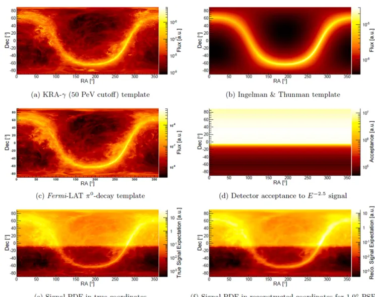
Figure 1.Three models for diffuse Galactic neutrino production described in Section2are shown in equatorial coordinates:(a) KRA-γ (50 PeV cutoff), (b) Ingelman & Thunman parameterization, and (c) Fermi-LAT p0_{-decay map. The models are followed by an illustration of the ps-template search technique described in}

Section3.1:(d) the detector acceptance for anE-2.5_{power law,(e) the distribution of neutrino events before and (f) after smearing due to the median PSF with the}

but visible from the northern sky. This is the region (  < <30 l 65 and -  < 2 b< 2 ) where Milagro is sensitive and used to tune the model. Note that the ARGO-YBJ (Bacci et al. 1999) experiment reports that gamma-rays between

∼350GeV and ∼2TeV are consistent with the Fermi-LAT model after masking out all sources(Bartoli et al.2015). If the

Milagro diffuse flux measurement above ∼1 TeV in the plane can be resolved into individual leptonic sources by HAWC, the KRA-γ predictions may need to be adjusted downward.

Finally, we also consider a smooth parameterization of the Galaxy from Ingelman & Thunman (1996). This model lacks

the detailed cosmic-ray modeling and mapping of the ISM of thefirst two models but captures the overall shape and structure of the Galaxy. The scale height of the Galaxy is also higher than the Fermi-LAT or KRA-γ models. Though this model is cruder than the others, we view it as valuable to include since it gives us robust results that only depend on simple assumptions. The model assumes that pure-proton cosmic rays are uniformly distributed throughout the entire volume and that the normalization and spectrum match that observed at Earth. The ISM extends out to a radius of 12 kpc with a density of

- ( )

e

1.0 h 0.26 kpc _{nucleon cm}−3_{, where h is the height out of the} Galactic plane in either direction. From simulations, we find that the model predicts 248 neutrino events in the 7 year muon sample afterfinal event selection. Even with the higher number of events than the other models, these neutrinos follow anE-2.7 spectrum up to the cosmic-ray knee and softening to E-3.0 above that, which is closer to the atmospheric background spectrum than the other models. This spectral information is fixed in the analysis of this model. Note that this prediction now takes neutrino oscillations, which the model predates, into account.

2.2. Catalogs for Stacking

Five different Galactic catalogs, each containing 4–10 sources described in Table1, were examined with the standard point-source stacking technique seen in Abbasi et al. (2011).

The sources were grouped into smaller catalogs under the assumption that the sources within each category would have similar properties, such as spectral index. This is important, as the spectral index, although a free parameter in the analysis, is assumed to be the same for all sources in each catalog. These catalogs are based on results from Milagro(Atkins et al.2004),

HAWC(Abeysekara et al.2013), and those compiled by SNR

Cat(Ferrand & Safi-Harb2012).

The HAWC catalog consists of 10 sources observed by HAWC after collecting thefirst year of data in the inner Galactic plane Abeysekara et al.(2016). This catalog was inspired by the

large overlap in sensitive energy range between the HAWC and IceCube detectors, permitting a multimessenger view of the same candidate astrophysical particle accelerators.

The Milagro catalog contains six Milagro sources in the Cygnus region originally reported by Abdo et al. (2007) and

modeled in Kappes et al. (2009) and Gonzalez-Garcia et al.

(2009) as possible PeVatron candidates. This catalog has been

used for stacking analysis previously using four years of IceCube data where a 2% p-value was found (Aartsen et al.

2014c). This analysis updates these results by adding an

additional three years of data.

Thefinal three catalogs are sub-catalogs of a group of SNRs taken from SNR Cat that have been observed in the TeV region with ages less than 3000years. The selection of young SNRs

was inspired by results demonstrating that SNRs less than 3000years old are more efficient accelerators in the TeV region (de Naurois 2015). This group was then divided into

three subgroups of sources based on their observed environ-ment: those with known molecular clouds, those with associated PWNe, and those with neither.

3. Analysis Methods

Maximum likelihood techniques are widely used in neutrino astronomy, and all analyses presented here use variations on existing methods. The stacking method used to search the catalogs in Section 2.2 is fully described in Abbasi et al. (2011). The spatial template methods are newer and described

below.

3.1. PS-template Analysis

The ps-template analysis method is a modification of the unbinned maximum likelihood analysis commonly employed in IceCube collaboration point-source searches (Braun et al.2008; Aartsen et al.2017a). The analysis uses an

event-wise point-spread function(PSF). While the angular resolution of our best reconstructed events is small(~ 0 . 1) compared to the spatial structures of the Galactic plane, accounting for the PSF of our less well reconstructed events(~ 3 . 0) is important. The first modification is to account for the extension of the source by mapping the changing detector acceptance and convolving the true source hypothesis with the PSF of the events(in contrast to the delta-function source hypothesis used in point-source searches). The other modification relates to the estimate of the background using data. In a point-source analysis, a hypothetical source has a very small contribution in the declination band and is treated as negligible for determining the background. For the Galactic plane, the signal may extend over the entire sky and is no longer negligible. We construct a signal-subtracted likelihood that acknowledges this contrib-ution, making a small correction to the method introduced in Aartsen et al.(2015c).

As in Aartsen et al.(2017a), the mixture model likelihood is

defined as



where ns is the number of signal events for a flux following

spectral indexγ; N is the total number of events in the sample;

s g

(x )

Si i, i,Ei; is the signal probability distribution function (PDF) for event i at equatorial coordinatesxi = (a di, i)with a Gaussian PSF of width si and energy proxy Ei; and Bi is the

background PDF. In this case, the background PDF does not come directly from the observed data, which are now treated as a mixture of signal and background:

d = d +⎜⎛ - ⎟ d ⎝ ⎞ ⎠ ˜ ( ) ˜ ( ) ( ) ( ) D E n NS E n N B E

sin , sin , 1 sin , .

2

i i i s i i i s i i i

The ˜D and ˜S terms are constructed by integrating the events in

the event density as a function of sind and E for the experimental data and simulated signal, respectively. Solving for Bi and substituting into Equation (1), this gives the final

signal-subtracted likelihood function as



Though the signal and background PDFs are defined event-wise, in practice, events in the same stable data taking periods are grouped together to construct the signal and back-ground PDFs.

The Si terms, which encode information about both the raw

signal expectation and the detector performance, are constructed as follows. Starting with a model for how the neutrino flux is distributed across the sky, we perform a bin-by-bin multiplication with the effective area to obtain the expected number of neutrinos per unit solid angle in the sample as a function of the direction and energy. The effective area is determined using detailed simulations, described in Aartsen et al.(2016). Then the map is convolved with the PSF of the

event, which is adequately described by a Gaussian distribu-tion of width siestimated for each event and ranging from 0°.1 to 3°.0. In practice, maps are convolved in steps of 0°.1 over this range. These steps are illustrated in Figure1, integrating over energy for the case of a Galacticflux following anE-2.5 power law.

Table 1

Source Information for the Five Stacked Catalogs

Catalog Associated Names R.A(°) Decl.(°) Extensionσ (°) Age(years)

Milagro Sixa MGRO J1852+01 283.12 0.51 0.0 L

MGRO J1908+06 286.68 6.03 1.3 L MGRO J2019+37 304.68 36.70 0.64 L MGRO J2032+37 307.75 36.52 0.0 L MGRO J2031+41 307.93 40.67 1.5 L MGRO J2043+36 310.98 36.3 1.0 L HAWCb HWC J1825−133 276.3 −13.3 0.5 L HWC J1836−090c 278.9 −9.0 0.5 L HWC J1836−074c 279.1 −7.4 0.5 L HWC J1838−060 279.6 6.0 0.5 L HWC J1842−046c 280.5 −4.6 0.5 L HWC J1844−031c 281.0 −3.1 0.5 L HWC J1849−017c 282.3 −1.7 0.5 L HWC J1857+023 284.3 2.3 0.5 L HWC J1904+080c 286.1 4.44 0.5 L HWC J1907+062c 286.8 6.2 0.5 L

SNR with mol. cloudc Tycho 6.33 64.15 0 443

IC443 94.3 22.6 0.16 3000

SN 1006 SW 225.7 −41.9 1.06 1009

HESS J1708−410 258.4 −39.8 1.36 1000

HESS J1718−385 259.5 −37.4 0.15 1800

Galactic Center Ridge 266.4 −29.0 0.2 1200

HESS J1813−178 274.5 −15.5 0.77 2500 HESS J1843−033 281.6 −3.0 0 900 SNR G054.1+00.3 292.6 18.9 0 2500 Cassiopeia A 350.9 58.8 0 316 SNR with PWNc Crab 83.6 22.01 0 961 RX J0852.0−4622 133.0 −46.3 0.7 2400 MSH 15−52 228.6 −59.1 0.11 1900 HESS J1634−472 249.0 −47.3 0.63 1500 HESS J1640−465 250.3 −46.6 0.87 1000 SNR G000.9+00.1 266.8 −28.2 0 1900 HESS J1808−204 272.9 −19.4 0.14 960 HESS J1809−193 273.4 −17.8 0.92 1200 HESS J1825−137 278.4 −10.6 1.63 720 SNR alonec RCW 86 220.8 −62.5 0.98 2000 HESS J1641−463 250.3 −46.3 0.62 1000 RX J1713.7−3946 258.5 −38.2 0.65 350 HESS J1858+020 284.5 2.2 0.08 2300

Notes.The stacking method uses a Gaussian distribution to represent either the source shape or the localization uncertainty.

a

Kappes et al.(2009).

b

Abeysekara et al.(2016).

c_{Ferrand & Safi-Harb (}

A nested log-likelihood ratio between the best-fit signal strength and the null hypothesis(no Galactic signal) is used to construct the test statistic. Under the null hypothesis and in the large sample limit the test statistic follows a half-c2 -distribu-tion as expected (Cowan et al. 2011). Final upper limits,

sensitivities (given as median upper limits) and significances, such as the p-value of the experimental test statistic, are always calculated from scrambled data. We use a strict 90% upper limit construction(Neyman1937).

The data sample used by the ps-template and the stacking searches is described in Aartsen et al.(2017a). It is an all-sky

sample that spans 7 years with a total live time of 2431 days and 730,130 events. Some of the data were collected during the construction phase of IceCube with the partially completed detector. The sensitivity comes primarily from the northern sky, where IceCube sees a wide energy range of neutrino-induced muons. Though the sample extends into the southern sky, the sensitivity here is limited to very high energies because the energy selection and veto techniques that were used reject the softer background of down-going muons from cosmic-ray air showers. For the benchmark case of anE-2.5_{spectrum, the} energy range that contains 90% of signal events in the final event sample is 400 GeV to 170 TeV and the median PSF is 0°.79.

3.2. Diffuse-template Analysis

The binned maximum likelihood analysis is an extension of the analysis presented in Aartsen et al. (2016). There, the

contributions from conventional atmospheric neutrinos(Honda et al. 2007), prompt atmospheric (Enberg et al. 2008), and

isotropic astrophysical neutrinos, assuming a power-law energy spectrum, arefitted to experimental data. The events are binned according to the reconstructed zenith angle and an energy proxy. The resulting histograms are analyzed using a maximum likelihood approach. Differing from Aartsen et al.(2016), each

bin is modeled by a Poissonian likelihood function:

q x = -m q x m ( ) · ! ( ) ( ) L e k , , 4 i i k , i

where q=q(Fastro,gastro, ...) describe the signal parameters (i.e., properties of the astrophysical fluxes) and x describe the nuisance parameters. The expected number of events in bin i,

m_i, is given by the sum of the four flux expectations for the conventional, isotropic astrophysical, prompt, and

Galacticflux: q x m m x x m g x m x x m x = + F + + F ( ) ( ) ( ) ( ) ( ) ( ) , , , , , , . 5 i i i i i conv conv det astro

astro astro det prompt

prompt det

Galactic

Galactic det

Here x_conv and x_prompt refer to nuisance parameters, taking into account the theoretical uncertainties on the respectivefluxes. The atmospheric neutrinofluxes have been corrected for the cosmic-ray knee following the prescription in Aartsen et al.(2014a). We

include nuisance parameters that account for the choice of the primary cosmic-ray model and uncertainties in the cosmic-ray spectral index. Additionally, we include nuisance parameters to account for uncertainties in the calculation of the atmospheric neutrinofluxes, namely normalization and the kaon/pion ratio.

x_det refers to nuisance parameters taking into account detector uncertainties. For more information on those parameters we refer to Aartsen et al. (2016). The final, global likelihood is the

product of all per-bin likelihoodsL= _i Li.

Compared to Aartsen et al.(2016), this analysis is extended

by including the reconstructed right ascension, thus changing the histograms from two to three dimensions. Additionally, a template for the Galactic contribution, mGalactic, is added to the fit. Note that for the Fermi-LAT p0_{-decay template, the} expected Galactic neutrino flux also depends on the Galactic spectral index.

In contrast to the method described in the previous section, this method models the expected contributions of every flux component using Monte Carlo simulations. This allows us to see how the isotropic component changes with the best-fit Galactic component. The test statistic is defined as a log-likelihood ratio in the same fashion as the previous method, with the same limit and significance calculations.

The data sample for the diffuse-template analysis is described in Aartsen et al. (2016). Compared to the previous

method, the sample has a significantly higher purity of >99.7%, with comparable effective area and a slightly improved PSF. The sample is, however, limited to the northern hemisphere where the high neutrino purity standards can be achieved. The time period is somewhat shorter, as this selection does not apply to thefirst year when IceCube had just 40 of the final 86 strings deployed. The data set spans 6 calendar years with a total live time of 2060 days and 354,792 events. For the benchmark case of an E-2.5 _{spectrum, the energy range that} contains 90% of signal events in the final event sample is 420 GeV to 130 TeV and the median PSF is 0°.69.

Table 2

Summary of Results for both Galactic Plane Analysis Methods for Each of the Three Models

ps-template Method Diffuse-template Method

Spatial Template ns p-value Sensitivity f90% Upper Limit f90% p-value Sensitivity f90% Upper Limit f90%

Fermi-LAT p0_-decay,E-2.5 _{149 37% 2.97×10}−18 _{3.83×10}−18 _{7.0% 3.16×10}−18 _{6.13×10}−18

KRA-γ (50 PeV) 98 29% 79% 120% 6.9% 95% 170%

Ingelman & Thunman 169 41% 220% 260% 19.8% 260% 360%

Note.Best-fit number of signal events ns. Fluxes are integrated over the full sky and parameterized as fd nm+n¯m dE=f90%· (E 100 TeV)-2.5GeV−1cm−2s−1with

4. Results

4.1. Constraints on Diffuse Emission in the Plane The sensitivities and results of spatial template analyses are summarized in Table 2. Some excess from the Galaxy is observed in all cases, though it is not statistically significant. Because of the better sensitivity, the ps-template method was assigned, in advance of unblinding the data, to be the main result. The diffuse-template method acts as a cross-check. The systematic uncertainty on theflux in the case of the ps-template analysis is estimated to be 11% based on Aartsen et al.(2017a).

For the diffuse-template, the systematic uncertainty is included directly in the method. The upper limit for the KRA-γ test is shown in Figure2in comparison to the ANTARES upper limit, the KRA family of predictions, and the isotropic diffuse neutrino flux.

The Galactic excesses are somewhat larger and more significant for the diffuse-template cross-check, and this difference was investigated carefully for the benchmark

p0_{-decay template where the 7% p-value was found. Part of} the difference comes from the additional year of data used by the ps-template method. If we restrict this method to the same time period, the p-value drops from 37% to 22%. Running the ps-template method on the sample used by the diffuse-template method yields a p-value of 21%. Due to the purity requirement of the diffuse-template method, a check of the diffuse-template method on the alternative data set is not possible.

The spectrum of the signal neutrinos is given by the model in the cases of KRA-γ and Ingelman & Thunman, but we test a

range of spectral hypotheses using the p0_{-decay spatial} template. For a flux µE-g, the spectral index range that we test is quite broad,1 <g<4. This is a wider range than we would expect in our standard models. However, it matches the range used in previous point source and stacking searches and allows for unexpected contributions, such as an unresolved population of hard or soft spectrum sources. The results of this coarse scan in spectral index are given in Table3. The small, best-fit Galactic component has a slight preference for E-2.0 compared to E-2.5_{, consistent with the results of the} cross-check shown in the next section.

4.2. 2D Likelihood Scan and Implications for the Isotropic Astrophysical Flux

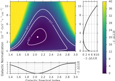
Using the diffuse-template method, a two-dimensional profile-likelihood scan of the Galactic normalization and Galactic spectral index is performed for the benchmark Fermi-LAT p0_{-decay template. The results of this scan are} shown in Figure 3. The best-fit spectral index is

g_Galactic= 2.07, and the best-fit flux (nm+n¯ ) normalizationm at 100 TeV is FGalactic =3.13·10-18GeV−1cm−2s−1. The confidence contours have been estimated using Wilks’ Theorem(Wilks1938), whose applicability has been confirmed

at several points in the parameter space with Monte Carlo

Figure 2.Upper limits at the 90% confidence level on the three-flavor (1:1:1 flavor ratio assumption) neutrino flux from the Galaxy with respect to KRA model predictions and the measured astrophysicalflux. Fluxes are integrated over the whole sky for uniform comparison. The IceCube 7-year upper limit for the KRA-γ (50 PeV) model test for the ps-template method is shown in red. The energy range of validity is from 1 to 500TeV. This range is calculated by finding the low- and high-energy thresholds where removing simulated signal events outside these values decreases the sensitivity by 5% each. The ANTARES limit in blue(Adrián-Martínez et al.2016a), directly applicable in

the Galactic center region (-  < <40 l 40 and -  <3 b< 3), has been scaled to represent an all-sky integrated flux for comparison. Due to ANTARES being located in the northern hemisphere, it has a relatively high sensitivity in the southern sky near the Galactic center region using muon neutrinos. The range of predictions for all the KRA models (Gaggero et al.2015) is shown as the gray band, with the top of that band representing

the KRA-γ (50 PeV) model. The model by Ingelman & Thunman (Ingelman & Thunman1996) is shown in purple. For comparison, measurements of the

all-sky diffuseflux are shown: a differential unfolding (black points) and a power-law unfolding(yellow band) of combined IceCube data sets from Aartsen et al. (2015a), as well as a measurement based only on northern sky muon data

(green band), from Aartsen et al. (2016).

Table 3

Summary of Results for the ps-template Analysis Scan in Spectral Index Using the Fermi-LAT p0_{-decay Spatial Template and Power-law Flux µE}-g

γ ns p-value Sensitivity f_90% Upper Limit f_90%

Softest: 4.0 13 45% 5.53×10−21 6.03×10−21 3.5 0 48% 7.27×10−20 7.27×10−20 3.0 15 49% 7.20×10−19 7.30×10−19 2.5 149 37% 2.97×10−18 3.83×10−18 2.0 103 24% 2.50×10−18 4.10×10−18 1.5 2 47% 3.79×10−19 3.79×10−19 Hardest: 1.0 0 76% 1.04×10−20 1.04×10−20 Note.Best-fit number of signal events ns. Fluxes are integrated over the full sky

and parameterized as fd nm+n¯m dE=f90%· (E 100 TeV)-g GeV

−1_cm−2_s−1

with 90% confidence level upper limits and median sensitivities quoted for f90%.

Figure 3.2D likelihood scan of spatially integrated Galacticflux (nm+n¯m)

normalization and Galactic spectral index. The marginal curves show the respective one-dimensional profile likelihoods. A change in -2·DLLH of 1 corresponds to the 1σ range.

pseudo-experiments. The best-fit spectral index is found to be somewhat harder than expected from gamma-ray observations. However, it is consistent with an index of 2.5 (2.7) at the 1.6 (2.1) σ-level.

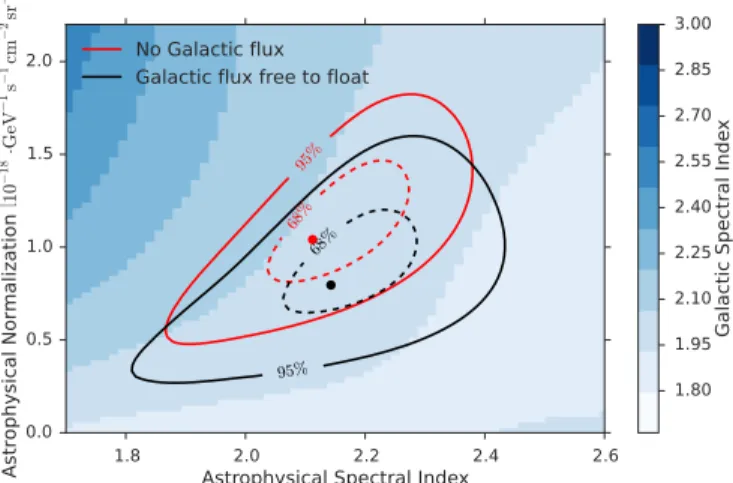
Since the diffuse-template method is an extension of the method used to characterize the isotropic astrophysicalflux in (Aartsen et al.2016), we can analyze the impact of allowing an

additional Galactic component in the fit on the isotropic flux parameters. For this we perform a profile-likelihood scan of the isotropicflux normalization and spectral index while allowing the Galacticflux parameters to float freely at every scan point. Figure4shows the resulting likelihood contours in comparison to the contours obtained by restricting the Galacticflux to zero. The color scale shows the best-fit Galactic plane spectral index at each point in the scan. Although the additional freedom given by the Galactic flux nuisance parameter causes the isotropic normalization to decrease, the size of the contour grows only marginally. The hypothesis of zero isotropicflux is still excluded at 3.8 . This shows that the observation of ans isotropic astrophysical signal is robust against a signal from the Galactic plane and that the latter can only contribute a sub-dominant fraction to the total observed extraterrestrial flux.

4.3. Constraints on Source Catalogs

The results from the stacking analyses are shown in Table4. All catalogs are consistent with small and statistically insignificant excesses. The most significant result with a p-value of 25% is the case of SNRs with molecular clouds, which gives just 16.5 excess events and a very soft spectral index close to the limit of g <4.0. Three of thefive catalogs have a very soft best-fit γ, which is expected since it is close to the atmospheric background. Compared to the results of Aartsen et al. (2015a) the all-sky integrated upper limit

assuming an E-2.5 _{spectrum for all of these catalogs is found} to be between 4 and 5 orders of magnitude below thefit for the isotropic diffuseflux.

The most promising Galactic catalog for stacked analysis was that of the six Milagro sources. The previous iteration of this search gave a p-value of 2% (Aartsen et al. 2014c). The

two sources MGROJ1908+06 and MGROJ2019+37 in this catalog are also two of the most significant of 74 individual

source candidates investigated as part of the 7-year IceCube source list search (Aartsen et al.2017a). Their respective

pre-trial p-values are 0.025 and 0.23. However, the results of this search for the six Milagro sources showed a decrease in significance from a p-value of 2%–29%. This result excludes the model of Kappes et al. (2009), based on Milagro

observations, with more than 95% confidence. Given that MGROJ1908+06 and MGROJ2019+37 are two of the most significant results from the source list search in Aartsen et al. (2017a), we investigated the apparent discrepancy. In contrast

to the source list search, this stacked analysis used source extensions on the order of 1°, as reported by Milagro (Abdo et al. 2007). The coordinates for this stacking analysis come

from the Milagro data as opposed to those found by Fermi-LAT. While the latter are better localized, the former come directly from >1TeV gamma-rays, which are a better match for the IceCube energy range. The combination of these effects on the strongest source alone, MGROJ1908+06, results in a substantial significance decrease, from a p-value of 4.6%–47%.

5. Conclusions

We have presented searches for neutrino signals associated with the Galactic plane using seven years of IceCube muon neutrino data, focusing on diffuse emission from interactions of cosmic rays with the ISM. We are able to exclude the possibility that more than 14% of the isotropic diffuse neutrino flux as measured in Aartsen et al. (2015a) comes from the

Galactic plane for the case of the Fermi-LAT p0_-decay template and an E-2.5 _{power law. This assumes the flux} continues down in energy to 1TeV or less, as would be expected for the case of cosmic-ray interactions with the ISM. The astrophysical neutrinoflux has only been measured above 10TeV so far, and its diffuse-template fit parameters are not changed significantly when the fit includes a Galactic component.

Our measurement is primarily sensitive in the northern hemisphere, where IceCube has a high efficiency for a wide energy range of muons induced by neutrinos. Our limits are quoted assuming various all-sky spatial models of neutrino emission. The KRA family of models spans a wide range and implies that a Galactic neutrino contribution must be present at some level. The most optimistic KRA-γ with a 50PeV cosmic-ray cutoff concentrates the most flux toward the Galactic center. Even though a higher fraction of the flux is in the southern sky, our limits are just 20% higher than this model prediction. In principle, if even more flux were concentrated near the Galactic center than in KRA-γ, it could be missed in this analysis and the limits would be violated. However, it is difficult for this to happen without overproducing gamma-rays (Gaggero et al. 2015; Kistler 2015). One way to circumvent

this is if production occurs very near SgrA* where the environment may be opaque to gamma-rays(Kistler2015). The

ANTARES detector also sets relevant constraints measured directly in the region surrounding the Galactic center (-  < <40 l 40 and -  < 3 b< 3 ). They limit the neutrino flux to be less than 60% higher than the KRA-γ model at 100TeV (Adrián-Martínez et al.2016a).

A blind search both for individual point sources and for multiple sub-threshold hotspots in the plane has previously been performed and sets constraints on the contribution of a small number of localized sources(Aartsen et al.2017a). The

stacking analysis presented here improves these results for

Figure 4.Contours of isotropic astrophysicalflux (nm+n¯m) normalization and

spectral index with and without Galactic flux in the fit. The case with no Galacticflux differs a small amount from Aartsen et al. (2016) because of the

several catalogs where the source locations are known. The catalog results are all of low significance and allow us to exclude the model of Kappes et al. (2009). Newer models

motivated by more recent gamma-ray observations predict a lowerflux with softer indices (Gonzalez-Garcia et al.2014).

While ourflux constraints focus on the plane of the Galaxy, there are still possibilities for the flux to originate in or very near the Galaxy. The possibility of cosmic-ray interactions with a gas halo extending out to ∼100kpc is still being actively explored(Feldmann et al.2013; Taylor et al.2014; Kalashev & Troitsky2016). Another possibility is the annihilation (Aartsen

et al.2015c; Albert et al.2017) or decay (Murase et al.2015) of

dark matter particles in the Galactic halo. For these hypotheses, the emission is much more isotropic than the Galactic emission templates that we tested.

There are possibilities to improve the sensitivity for Galactic neutrino searches. A search for point sources in the Southern hemisphere using cascade-like events in IceCube has been shown to have a sensitivity comparable to ANTARES. Though cascades have a much larger median PSF (between 11° and 20°), the angular resolution matters less in the case of a large-scale, spatially extended source such as the galactic plane. Cascade-like events also have a lower energy threshold in the southern sky compared to muons(Aartsen et al.2017c). A joint

analysis that includes both the track and cascade channels will offer promising improvements. Additionally, a joint Galactic plane analysis between IceCube and ANTARES, similar to the joint point-source analysis that produced better limits in the southern sky (Adrián-Martínez et al. 2016b), would provide

the strongest constraints on neutrinos from the Milky Way with all available data.

We acknowledge the support from the following agencies: U.S. National Science Foundation-Office of Polar Programs, U.S. National Science Foundation-Physics Division, University of Wisconsin Alumni Research Foundation, the Grid Labora-tory Of Wisconsin (GLOW) grid infrastructure at the University of Wisconsin—Madison, the Open Science Grid (OSG) grid infrastructure; U.S. Department of Energy, and National Energy Research Scientific Computing Center, the Louisiana Optical Network Initiative (LONI) grid computing resources; Natural Sciences and Engineering Research Council of Canada, WestGrid and Compute/Calcul Canada; Swedish Research Council, Swedish Polar Research Secretariat, Swedish National Infrastructure for Computing (SNIC), and Knut and Alice Wallenberg Foundation, Sweden; German Ministry for Education and Research (BMBF), Deutsche Forschungsgemeinschaft(DFG), Helmholtz Alliance for Astro-particle Physics(HAP), Initiative and Networking Fund of the Helmholtz Association, Germany; Fund for Scientific Research

(FNRS-FWO), FWO Odysseus programme, Flanders Institute to encourage scientific and technological research in industry (IWT), Belgian Federal Science Policy Office (Belspo); Marsden Fund, New Zealand; Australian Research Council; Japan Society for Promotion of Science (JSPS); the Swiss National Science Foundation (SNSF), Switzerland; National Research Foundation of Korea(NRF); Villum Fonden, Danish National Research Foundation(DNRF), Denmark.

ORCID iDs A. Christov https://orcid.org/0000-0001-8121-5860 S. Coenders https://orcid.org/0000-0002-1556-025X J. J. DeLaunay https://orcid.org/0000-0001-5229-1995 P. Desiati https://orcid.org/0000-0001-9768-1858 G. de Wasseige https://orcid.org/0000-0002-1010-5100 P. A. Evenson https://orcid.org/0000-0001-7929-810X J. Gallagher https://orcid.org/0000-0001-8608-0408 U. Katz https://orcid.org/0000-0002-7063-4418 A. Keivani https://orcid.org/0000-0001-7197-2788 S. Schoenen https://orcid.org/0000-0002-9236-6151 M. Sutherland https://orcid.org/0000-0001-5204-1873 J. Vandenbroucke https://orcid.org/0000-0002-9867-6548 S. Westerhoff https://orcid.org/0000-0002-1422-7754 D. L. Xu https://orcid.org/0000-0003-1639-8829 References

Aartsen, M. G., Abbasi, R., Abdou, Y., et al. 2013,Sci,342, 1242856

Aartsen, M. G., Abbasi, R., Ackermann, M., et al. 2014a,PhRvD,89, 062007

Aartsen, M. G., Abraham, K., Ackermann, M., et al. 2015a,ApJ,809, 98

Aartsen, M. G., Abraham, K., Ackermann, M., et al. 2015b,PhRvL,115, 081102

Aartsen, M. G., Abraham, K., Ackermann, M., et al. 2015c,EPJC,75, 492

Aartsen, M. G., Abraham, K., Ackermann, M., et al. 2016,ApJ,833, 3

Aartsen, M. G., Abraham, K., Ackermann, M., et al. 2017,ApJ,835, 45

Aartsen, M. G., Ackermann, M., Adams, J., et al. 2014b,PhRvL,113, 101101

Aartsen, M. G., Ackermann, M., Adams, J., et al. 2014c,ApJ,796, 109

Aartsen, M. G., Ackermann, M., Adams, J., et al. 2017a,ApJ,835, 151

Aartsen, M. G., Ackermann, M., Adams, J., et al. 2017b,ApJ,843, 112

Aartsen, M. G., Ackermann, M., Adams, J., et al. 2017c,ApJ,846, 136

Aartsen, M. G., Ackermann, M., Adams, J., et al. 2017d,JInst,12, P03012

Abbasi, R., Abdou, Y., Abu-Zayyad, T., et al. 2010,NIMPA,618, 139

Abbasi, R., Abdou, Y., Abu-Zayyad, T., et al. 2011,ApJ,732, 18

Abbasi, R., Ackermann, M., Adams, J., et al. 2009,NIMPA,601, 294

Abdo, A. A., Allen, B., Berley, D., et al. 2007,ApJL,664, L91

Abeysekara, A., Alfaro, R., Alvarez, C., et al. 2013,APh,50, 26

Abeysekara, A., Alfaro, R., Alvarez, C., et al. 2016,ApJ,817, 3

Acero, F., Ackermann, M., Ajello, M., et al. 2016,ApJS,223, 26

Ackermann, M., Ajello, M., Albert, A., et al. 2012a,ApJS,203, 4

Ackermann, M., Ajello, M., Atwood, W. B., et al. 2012b,ApJ,750, 3

Adrián-Martínez, S., Albert, A., André, M., et al. 2016a,PhLB,760, 143

Adrián-Martínez, S., Albert, A., André, M., et al. 2016b,ApJ,823, 65

Albert, A., André, M., Anghinolfi, M., et al. 2017,PhLB,769, 249

Atkins, R., Benbow, W., Berley, D., et al. 2004,ApJ,608, 680

Bacci, C., Bao, K. Z., Barone, F., et al. 1999,A&AS,138, 597

Bartoli, B., Bernardini, P., Bi, X. J., et al. 2015,ApJ,806, 20

Table 4

Summary of Results for the Galactic Catalogs

Source Catalog Number of Sources p-value ns γ Upper Limit f_90%

Milagro Six 6 30% 31.8 3.95 3.98×10−20

HAWC Hotspots 10 31% 17.3 2.38 9.48×10−21

SNR with mol. clouds 10 25% 16.5 3.95 2.23×10−19

SNR with PWN 9 34% 9.36 3.95 1.17×10−18

SNR alone 4 42% 3.82 2.25 2.06×10−19

Note. ns andγ are the best-fit numbers of signal events and spectral index, respectively. Fluxes are given as the sum over the catalog and parameterized as

f_n+n =f

-m ¯m · ( )

d dE _90% E 100 TeV 2.5_GeV−1_cm−2_s−1_{with 90% confidence level upper limits quoted for f} 90%.

Bechtol, K., Ahlers, M., Di Mauro, M., Ajello, M., & Vandenbroucke, J. 2017, ApJ,836, 47

Braun, J., Dumm, J., De Palma, F., et al. 2008,APh,29, 299

Clark, G. W., Garmire, G. P., & Kraushaar, W. L. 1968,ApJL,153, L203

Cowan, G., Cranmer, K., Gross, E., & Vitells, O. 2011,EPJC,71, 1554

de Naurois, M. 2015, Proc. ICRC(The Hauge, The Nertherlands),34, 21

Enberg, R., Reno, M. H., & Sarcevic, I. 2008,PhRvD,78, 043005

Feldmann, R., Hooper, D., & Gnedin, N. Y. 2013,ApJ,763, 21

Ferrand, G., & Safi-Harb, S. 2012,AdSpR,49, 1313

Gaggero, D., Grasso, D., Marinelli, A., et al. 2015,ApJL,815, L25

Gonzalez-Garcia, M. C., Halzen, F., & Mohapatra, S. 2009,APh,31, 437

Gonzalez-Garcia, M. C., Halzen, F., & Niro, V. 2014,APh,57, 39

Honda, M., Kajita, T., Kasahara, K., et al. 2007,PhRvD,75, 043006

Ingelman, G., & Thunman, M. 1996, arXiv:hep-ph/9604286

Kalashev, O., & Troitsky, S. 2016,PhRvD,94, 063013

Kappes, A., Halzen, F., & Murchadha, A. Ó 2009,NIMPA,602, 117

Kistler, M. D. 2015, arXiv:1511.05199

Murase, K., Laha, R., Ando, S., & Ahlers, M. 2015,PhRvL,115, 071301

Neronov, A., & Malyshev, D. 2015, arXiv:1505.07601

Neronov, A., & Semikoz, D. 2016,APh,75, 60

Neyman, J. 1937,RSPTA,236, 333

Patrignani, C., Agashe, K., Aielli, G., et al. 2016,ChPhC,40, 100001

Taylor, A. M., Gabici, S., & Aharonian, F. 2014,PhRvD,89, 103003