Potential future lakes from continued glacier shrinkage in the Aosta
Valley Region (Western Alps, Italy)
Cristina Viani
a,⁎
, Horst Machguth
b,c, Christian Huggel
b, Alberto Godio
d, Diego Franco
d,
Luigi Perotti
a, Marco Giardino
aaDepartment of Earth Sciences, University of Torino, Italy bDepartment of Geography, University of Zurich, Switzerland c
Department of Geosciences, University of Fribourg, Switzerland
d
Department of Environment, Land and Infrastructure Engineering, Politecnico di Torino, Italy
Keywords: Glacier lakes Glacier shrinkage Glacier bed topography Western Italian Alps
Aosta Valley (Western Alps, Italy) is the region with the largest glacierized area of Italy. Like other high mountain regions, it has shown a significant glacier retreat starting from the end of the ‘Little Ice Age’ that is expected to continue in the future. As a direct consequence of glacier shrinkage, glacier-bed overdeepenings become exposed, offering suitable geomorphological conditions for glacier lakes formation. In such a densely populated and devel-oped region, opportunities and risks connected to lakes may arise: 1) economic exploitation for hydropower production, tourism and water supply; 2) environmental relevance for high mountain biodiversity and geodiversity; 3) potential risks due to outbursts and consequent floods.
In this study, the locations of potential future glacier lakes over large glacierized areas (183 glaciers covering 163,1 km2) of Aosta Valley were assessed by using the GlabTop2 model.
46 overdeepenings larger than 10,800 m2 were identified, covering an area of 3.1 ± 0.9 km2 and having a volume
of 0.06 ± 0.02 km3. The majority of the overdeepenings are located in the Monte Rosa-Cervino massif and a mean
depth b10 m characterizes them. Moreover, an estimation of the most recent total ice volume for the Aosta Valley was provided (5.2 ± 1.6 km3 referred to 2008).
Thanks to the validation by the proposed “backward approach” and GPR (Ground Penetrating Radar) data, we can confirm that the location of the overdeepenings is robust while their actual dimensions are subject to consid-erable uncertainties. Almost all of large lakes (area N 10,000 m2), potentially the most dangerous, are modelled.
Finally, we suggest choosing medium pixel size (about 60 m) of the DEM in order to obtain, at least, the location of the largest lakes and to avoid overestimations of ice thickness and thus a great number of false positive overdeepenings.
The results presented here can be useful for understanding how the alpine environment will look in the future and can help the management of water resources and risks related to glacier lakes.
1. Introduction
It is expected that the rapid retreat of glaciers, observed in the European Alps and other mountain regions of the world, will continue in the future (Zemp et al., 2006;IPCC, 2013;Zekollari et al., 2019). One of the most evident and relevant consequences is the formation of new glacier lakes in recently deglaciated areas (Linsbauer et al., 2009;Buckel et al., 2018). During glacier retreat, overdeepenings, defined byHaeberli et al. (2016b)as“closed topographic depressions with adverse slopes in theflow direction, characteristic for glacier beds and glacially sculpted
landscapes”, become exposed and, in some cases, filled with water rather than sediments. Glacier-bed geomorphologic processes involved in shaping overdeepenings are mainly basal sliding and bedrock abrasion by iceflux, localized bedrock quarrying and the action of complex system of pressurized sub-glacial meltwater drainage (Fischer and Haeberli, 2012). The latter, in particular, is supposed to play a predominant role, both in affecting basal sliding and the efficiency of direct glacier-bed ero-sion, and in evacuating sediments keeping the bedrock accessible for fur-ther erosion (Haeberli et al., 2016b).
Progressive shrinkage of glaciers is followed by an increasing num-ber of new glacier lakes (Paul et al., 2007;Carrivick and Tweed, 2013;
Mergili et al., 2013;Emmer et al., 2014;Salerno et al., 2014;Viani et al., 2016) and by significant geomorphological changes (appearing/ disappearing, expansion/shrinkage) in the existing ones that reflect
⁎ Corresponding author at: Department of Earth Sciences, Via Valperga Caluso, 35, 10125 Torino, TO, Italy.
E-mail address:cristina.viani@unito.it(C. Viani).
http://doc.rero.ch
Published in "Geomorphology 355(): 107068, 2020"
which should be cited to refer to this work.
climaticfluctuations and environmental changes (Gardelle et al., 2011;
Salerno et al., 2014, 2016;Zhang et al., 2017).
When new lakes form because of glacier retreat, both opportunities and risks may arise (Haeberli et al., 2016a), due to several reasons: 1) the poten-tial economic value of glacier lakes for hydropower production, tourism ac-tivities and as water reservoir (Terrier et al., 2011;Purdie, 2013;Drenkhan et al., 2019); 2) their environmental relevance for high mountain biodiver-sity (Čiamporová-Zaťovičová and Čiampor, 2017;Tiberti et al., 2019) and geodiversity (Diolaiuti and Smiraglia, 2010); 3) the associated potential risks, e.g. lake outbursts and consequentfloods (Allen et al., 2009;Worni et al., 2013;Emmer et al., 2015, 2016).
The scientific interest and importance of these geomorphologic fea-tures is demonstrated by the high number of regional glacier lake inven-tories produced for many high mountain regions of the world since the beginning of the XXI century. The majority of the studies refers to high mountain Asia: the Himalaya region (Gardelle et al., 2011;Worni et al., 2013;Zhang et al., 2015;Salerno et al., 2016), Mount Everest (Wessels et al., 2002;Bolch et al., 2008;Tartari et al., 2008;Salerno et al., 2012), the Tibetan Plateau (Zhang et al., 2017), Tien Shan (Bolch et al., 2011) and Bhutan (Komori, 2008). There are also examples in South America, across the Andes (Loriaux and Casassa, 2012;Hanshaw and Bookhagen, 2014;Emmer et al., 2016;Drenkhan et al., 2018). Some studies refer to Iceland (Schomacker, 2010), Alaska (Capps and Clague, 2014) and the Caucasus (Stokes et al., 2007). Concerning the European Alps, studies were conducted in Switzerland (Huggel et al., 2002;Paul et al., 2007;
Frey et al., 2010b), Austria (Emmer et al., 2015;Buckel et al., 2018) and Italy (Galluccio, 1998;Salerno et al., 2014;Viani et al., 2016).
More recently, the necessity has emerged of detecting and assessing location of future potential glacier lakes. Several studies presented ap-proaches for modelling location and morphometric characteristics of possible future lakes applied in some mountain regions of the world such as: Switzerland (about 500 potential new lakes modelled by
Linsbauer et al., 2012); Himalaya-Karakoram (16,000 overdeepenings reported in Linsbauer et al., 2016); the Peruvian Andes (201 overdeepenings identified byColonia et al., 2017); the Djungarskiy Alatau region in Central Asia (513 potential future lakes modelled by
Kapitsa et al., 2017); and the Mont Blanc massif (80 glacier-bed overdeepenings estimated byMagnin et al., 2020).
The assessment of the potential location of future lakes is possible through ice thickness modelling and the subsequent generation of a DEM (Digital Elevation Model) without glaciers (Linsbauer et al., 2009). Thereby, one assumes that future lakes form where the model predicts overdeepened areas (i.e.: overdeepenings) in the bedrock un-derneath existing glaciers. Results of these approaches were validated at the local scale (single glacier) through: i) the comparison of modelled ice thickness with measurements taken by in situ geophysical investiga-tions (e.g., Ground Penetrating Radar), which can be logistically and economically demanding (Farinotti et al., 2017); ii) the analysis of the location of modelled overdeepenings with respect to morphological criteria (Frey et al., 2010a;Colonia et al., 2017); iii) the application of models to historical data for comparing results with the present situa-tion (Frey et al., 2010a).
The goal of the present study is to assess the location of potential fu-ture lakes for the Aosta Valley Region, Western Italian Alps. The area has been selected for its wide glacier extension, thus being significant for providing information about future lakes (thefirst attempt in the Italian Alps) and adding information on this topic from a newly studied region of the European Alps. The results and the suitability of the model will be evaluated using further proposed ways (backward validation at the re-gional scale) in addition to those used in existing studies (forward vali-dation at the local scale).
Our specific objectives are:
- to give an estimation of the ice thickness and volumes of the Aosta Valley glaciers;
- to provide a map of possible future lakes for the region;
- to validate, through both well established and additional proposed ways, the suitability of the GlabTop2 model for modelling glacier-bed overdeepenings for mountain glaciers and for anticipating the formation of lakes;
- to test the sensitivity of the model on the input data.
2. Study region
The present study focuses on the glacierized areas of the Aosta Valley Region within the Western Italian Alps. The Aosta Valley is the region with the most extensive glacier cover in Italy. According to the new Italian Glacier Inventory (Smiraglia et al., 2015), related to the 2005–2011 pe-riod, 192 glaciers exist in the Aosta Valley Region with a cumulative area value of 133.7 km2, which corresponds to 36% of the Italian glacier area (21% with respect to the total number of glaciers). In 1991, year of the dataset used in the present research, there were 183 glaciers (N0.05 km2) covering 163.1 km2(Fig. 1). The number of glaciers was smaller but they covered a larger area if compared to 2005–2011. Differ-ences in number and area are due to ongoing disintegration of glaciers (from one larger, single glacier body to several smaller bodies) and shrinkage and disappearance that took place in the meantime (Salvatore et al., 2015).
The largest glaciers, according to the 1991 dataset, were Miage (13.6 km2), Lys (11.8 km2) and Rutor (9.3 km2).
The glaciers cover an elevation range from about 1400 m a.s.l. up to 4800 m a.s.l. and have a mean elevation of about 3000 m a.s.l. The 15 glaciers with an area larger than 3 km2contribute 54% to the total glacierized area but only 8% to the total number. On the contrary, gla-ciers smaller than 1 km2account for 80% of the number but only 23% for the area (Fig. 2). Most glaciers are mountain glaciers with few cases of valley glaciers (in 1991: Miage Glacier, Brenva Glacier, Lys Gla-cier, Verra Grande GlaGla-cier, Pre de Bar Glacier).
Within the study region,Viani et al. (2016)reported about 200 new glacier lakes being formed within‘Little Ice Age’ (LIA) glacier extent boundaries (by http://www.glariskalp.eu/ and referred to 1850.
Orombelli, 2011dated the LIA-maximum for the Western Alps in 1845–1860) covering an area of about 1.3 km2. About ¾ of these lakes are dammed by bedrock, the remaining are mainly dammed by sedi-ments. The 12 lakes with an area larger than 20,000 m2contribute 52% to the total lake coverage but only 6% to the total number. On the other hand, lakes smaller than 6000 m2account for 81% of the total number, but only 23% of the total area.
Glacier lakes represent both opportunities and risks in the study re-gion. As the Miage (Veny Valley) and Blue (Ayas Valley) lakes, some gla-cier lakes are important touristic attractions in addition to be valuable geosites (i.e. features showing a particular geological or geomorpholog-ical significance;Reynard, 2004). Some lakes are potentially hazardous, e.g. Rutor (Dutto and Mortara, 1992) and Miage (Diolaiuti et al., 2006) lakes. In this context, the recent lake outburst event of August 2016 at the Gran Croux lake above Cogne (Gran Paradiso group) is mentioned (FMS, 2016).
Besides its large number of glaciers and lakes, the Aosta Valley was chosen also for its large amount of data on this topic. Information about historical (Ajassa et al., 1994, 1997;CGI-CNR, 1961;Citterio et al., 2007;Diolaiuti et al., 2012;Giardino et al., 2017) and present (Smiraglia et al., 2015;Salvatore et al., 2015) glacier extent and surface elevation are available. These data are fundamental as input data for the modelling of bedrock topography underneath glaciers and the detection of possible overdeepenings. Existing and available glacier lakes invento-ries (Viani, 2018) and GPR data (Villa et al., 2008) are useful for validat-ing model results.
Three glaciers (Gran Etret, Indren and Rutor) were selected for vali-dation of the modelled glacier bed topography with GPR data:
1) Gran Etret Glacier (0.6 km2) is in the Gran Paradiso chain of the Graian Alps. It is a mountain glacier with a simple basin form and facing north. It lost about 75% of its LIA area (referred to 1850,
http://www.glariskalp.eu/).
2) Indren Glacier (1 km2) is a mountain glacier with a simple basin out-line, facing south and located in the Monte Rosa group in the Pennine Alps. The slope is quite steep, except the central part of the glacier. The glacier front retreated about 1 km after the
LIA-maximum (1850), 4 glacier lakes appeared dammed by the glacially modelled bedrock.
3) Rutor Glacier (9.1 km2in 1991) is located in the Rutor-Lechaud chain in the Graian Alps, facing northwest. It is the third largest glacier in Aosta Valley by area and has a ratherflat surface morphology. Rutor Glacier is divided into two main branches by a rocky ridge, the conjunction of the two branches is visible in the lower part of the glacier, down-valley of a rock outcrop where a medial moraine
Fig. 1. Map of the study region showing all Aosta Valley glaciers and all glacier lakes formed after the‘Little Ice Age’ (LIA) maximum (a). Abbreviations refers to the validation glaciers shown in the detailed maps: b) Rutor (RU), c) Gran Etret (GE) and d) Indren (IN).
forms. The glacier has a well-known history of a series of glacier lake outburstfloods between 1430 CE and 1864 CE due to front fluctua-tions (Orombelli, 2005). After the LIA-maximum (dated 1864 for the Rutor Glacier byOrombelli, 2005), 8 new lakes have formed dammed by moraines and in newly exposed overdeepenings (Villa et al., 2007).
3. Data and methods
Table 1summarizes the workflow of the present research as de-scribed in the following.
3.1. The GlabTop2 model
The GlabTop2 is part of the GlabTop approach (Linsbauer et al., 2009) developed for assessing the spatial distribution of ice thickness by esti-mating the glacier depths at several points within the glacierized areas. The GlabTop approach has been widely used for modelling potential
future lakes in many mountain regions of the world by using recent input data (e.g.Linsbauer et al., 2016;Colonia et al., 2017;Kapitsa et al., 2017).Linsbauer et al. (2012)applied GlabTop approach to historical data (glacier outlines from 1973 and a DEM from 1985) for Switzerland. The Glacier Bed Topography model version 2 (GlabTop2 model;Frey et al., 2014) is a fully automated model that requires a minimum set of input data: glacier outlines (glacier mask) and a surface DEM. It allows to model glacier bed topography over large areas combining digital ter-rain information and slope-related estimates of glacier thickness (Linsbauer et al., 2016). Consequently, the location of possible overdeepenings in the bedrock can be assessed.
Ice thickness h is calculated for an automated selection of randomly picked DEM cells within the glaciated area by using the following rela-tionship:
h¼ τ= f ρgsinαð Þ ð1Þ
τ is the basal shear stress, f the shape factor (related to the friction of a real glacier with the valley walls),ρ the ice density (900 kg m−3), g the acceleration due to gravity (9.81 m s−2) andα the surface slope measured over a given vertical interval (which is calculated by the model on randomly selected cells).
The calculation requires estimating the parametersτ and f. Accord-ing to previous works (Haeberli and Hoelzle, 1995;Linsbauer et al., 2016;Farinotti et al., 2017),τ is parameterized with the vertical extent of the entire glacierΔH by the equation inHaeberli and Hoelzle (1995). τ ¼ 0:005 þ 1:598ΔH−0:435ΔH2
ð2Þ FollowingLinsbauer et al. (2012), f is set to 0.8 for all glaciers which is typical for valley glaciers.
The model was run using the above-mentioned parameter settings identical to the original parameters used byFrey et al. (2014). The resulting ice thickness distribution was subtracted from the corre-sponding surface DEM to provide the bed topography of the investi-gated glaciers.
Farinotti et al. (2017), in the framework of the Ice Thickness Models Intercomparison eXperiment (ITMIX), compared the results of a set of 17 different models for 21 test cases. The results obtained by the use of GlabTop2 are comparable in quality with more complex model ap-proaches (e.g.:Farinotti et al., 2009;Huss and Farinotti, 2012). The model is limited in its ability to reproduce small-scale details and, in contrast to other models, performs poorly in modelling ice thickness of ice caps, but this is of no issue in the context of the present study.
3.2. Application to all Aosta Valley glaciers
We adopted the regional DEM of 1991 provided by the Regione Autonoma Valle d'Aosta (RAVA) with an original spatial resolution of 10 m, produced by aerial photogrammetry. We down-sampled the DEM to 60 m for the calculation using the bilinear interpolation algorithm, to avoid influence of small-scale surface morphologies on model outputs as suggested byFrey et al. (2014)andFarinotti et al. (2017). As glacier outlines we used the .kmlfile available from the GlaRiskAlp Project website (http://www.glariskalp.eu) and related to 1999. We modified and updated the outlines to the beginning of the 1990s, in order to have a goodfit with the 1991 DEM, by identifying glacier margin positions analysing the hillshade extracted from the 1991 DEM and available orthophotos of 1988–89. In order to avoid inaccurate results, glaciers smaller than 0.05 km2have been removed because they are subject to high uncertainties, as suggested byLinsbauer et al. (2016). Subsequently, glacier outlines have been converted to a rasterized glacier mask where all glacier grid cells receive unique IDs (one ID per glacier entity). We ap-plied the model to all the glaciers of the study region assessing,firstly, the ice thickness (step 1 inTable 1) and consequently the DEM of the bedrock underneath glaciers (step 2 inTable 1). Finally, we produced a database of
Fig. 2. Plot showing the glacier area and the number of glaciers with respect to the relative cumulative frequency of both values.
Table 1
Workflow of the present research.
Step Input data Method
1. Modelling glacier ice thickness
1991 glacier outlines 1991 DEM
Glacier Bed Topography Model 2 (Frey et al., 2014) 2. Calculation of bedrock topography and overdeepenings location 1991 DEM Ice thickness distribution (rasterfile)
ArcGis Toolbox (Linsbauer et al., 2012)
3. Backward validation at the regional scale
Modelled overdeepenings Lake inventories (Viani, 2018)
Comparison between modelled and real lakes in areas exposed by glacier retreat between 1991 and now
4. Backward validation at the local scale
Modelled bedrock Real bedrock (2008 LIDAR DTM)
Comparison between modelled and real bedrock along selected profiles for areas exposed by the glaciers after 1991
5. Forward validation at the local scale
Modelled bedrock GPR data on specific glaciers
Comparison between modelled and measured bedrock along selected profiles
6. Forward validation at the regional scale Modelled overdeepenings Orthophotos 1991 DEM
Morphological criteria (Frey et al., 2010a)
7. Sensitivity test 1991 DEM at different resolution
Repeat steps 1, 2, 3 and 5
the modelled overdeepenings (step 2 inTable 1) with associated morpho-metric parameters (area, depth, volume).
Finally, in order to estimate the most recent ice thickness and vol-ume of the Aosta Valley glaciers, we assvol-umed that bed topography modelled by GlabTop2 is independent from the date of the input data (DEM and glacier outlines). Ice thickness information have been ob-tained by subtracting the most recent regional elevation model (2008 LIDAR DTM of the Aosta Valley representing recent glacier surface ge-ometry) from the modelled bedrock without glaciers (i.e. the result of the GlabTop2 application to the 1991 data) and masking these results with the outlines from the most recent glacier inventory (2006–2007 glacier outlines fromSalvatore et al., 2015).
3.3. The backward approach
The main idea is to use historical datasets (glacier outlines and DEMs) as input data for the model. Steps 3 and 4, as presented in
Table 1, synthesizes the proposed backward approach.
Our approach is based on the assumption that glacier retreat was a general trend since the year of acquisition of the historical data. From the year at which the datasets refer (data survey) until now, in areas ex-posed from glacier ice, new glacier lakes appeared and glacially shaped landforms become exposed. Following a backward-looking procedure, existing glacier lake and freshly exposed glacially shaped landforms can be used to verify, at the regional scale, the correspondence with modelled lakes and to validate modelled bedrock, respectively. The ap-plication of the described approach requires a lake inventory and the availability of recent elevation models. In a GIS environment we evalu-ate whether locations of modelled overdeepenings correspond to the location of the newly formed lakes for the areas exposed by glacier ice. This approach should allow to test if glacier lakes formation can be predicted by GlabTop2.
Ideally, data from earlier time periods would be used to maximize glacier retreat since then. For this reason, we performed preliminary tests for the production of DEMs from historical aerial photogrammetry (aerial photos stereo pairs of the 1954 aerophotogrammetricflight) on selected glaciers where significant glacier lakes have formed in bedrock overdeepenings (e.g.: Rutor and Indren glaciers). The quality of the pho-tographs and the missing calibration certificate of the camera prevented an accurate evaluation of errors of the extracted orthophotos and DEMs. We also performed a real test with Structure for Motion (SfM) tech-nique with the same aerial photographs from 1954flight (Roberti et al., 2018) but the problem is that the number of photographs was in-sufficient to obtain a correct and accurate SfM model to compare with the regional 1991 DEM. In addition, the potential dataset produced would only cover single glaciers.
Thus, we decided to use the 1991 DEM dataset as input data because of its consistent data quality and the wide area covered. Furthermore, glacier lake inventories related to the end of the 1990s, 2006 and 2012 (Viani, 2018) exist and can be used to check the real presence of modelled lakes at the regional scale.
Finally, at the local scale (single glacier scale), focusing on areas sub-ject to glacier retreat since the 1990s, it is possible to compare their cur-rent topography with the modelled one along selected profiles. The regional 2008 LIDAR DTM of the Aosta Valley gives the recent topography.
3.4. The forward approach
In the existing literature (e.g.Linsbauer et al., 2012, 2016;Farinotti et al., 2017;Helfricht et al., 2019), researchers used geophysical investi-gations carried out on selected glaciers to validate model results.
We adopt a similar approach by performing a forward-looking vali-dation comparing Ground Penetrating Radar (GPR) profiles with modelled bedrock at the glacier scale (step 5 inTable 1). We consider several data sets: existing GPR data at Rutor and Gran Etret glaciers by
Villa et al. (2008)and by Regional Agency ARPA VDA in collaboration
with the Department of Environment, Land and Infrastructure Engi-neering (Politecnico di Torino), respectively. The data were acquired during differentfield campaigns (Rutor: 1996 and 2006, using a central frequency of 35 MHz; Gran Etret: 2013 by helicopter, using a main fre-quency of 70 MHz). A GPR survey was also carried out during summer 2016 (central frequency of 200 MHz) on the central area of Indren Gla-cier where GlabTop2 shows the presence of a possible subglacial overdeepening.
Moreover, the morphological criteria proposed byFrey et al. (2010a)
can be used as a forward validation at the regional scale (Colonia et al., 2017). For each modelled overdeepening of the study area it is possible, using orthophotos and DEMs, to verify if the morphological characteris-tics at sites where overdeepenings are modelled fulfil the mentioned criteria (step 6 inTable 1).
3.5. Sensitivity test on input data
In addition to the previously presented modelling with 60 m spatial resolution datasets, we performed additional runs of GlabTop2 varying the pixel size of the input data (DEM and glacier mask) from high to low spatial resolution: 20 m, 40 m and 90 m (step 7 inTable 1). The ob-jective is to evaluate the effect of the change of the pixel size on model results (ice thickness, bedrock geometry, total overdeepenings, depth and area), considering that GlabTop2 calculation of ice thickness is grid-based and that surface slope is derived as the average surface slope of all grid cells with a buffer of a given vertical elevation extent.
4. Results
4.1. Thickness and volume of the Aosta Valley glaciers
InFig. 3the ice thickness distribution, related to the year 2008, for all Aosta Valley glaciers is shown. Ice thicknesses lower than 50 m are dominant. 78% of the glaciers have a mean ice thickness below 25 m and another 18% between 25 and 50 m.
We estimated a total ice volume of 5.2 ± 1.6 km3for 2008 (for 1991 the total ice volume corresponds to 7.3 ± 2.2 km3), considering 30% as the uncertainty of the model as demonstrated byLinsbauer et al. (2012). The arithmetic mean ice thickness, obtained by dividing the total vol-ume by the total area, is about 39 m. Maximum modelled ice thickness is 214 m (Triolet Glacier).
Considering the volume of single glaciers, the 3, 9, and 27 largest gla-ciers (defined by volume) contained 28, 59 and 86% of the total volume of glaciers in the Aosta Valley, respectively. The three largest glaciers thereby are Miage (0.53 km3), Rutor (0.50 km3) and Lys (0.45 km3) gla-ciers. The thickest ones (considering the mean thickness) are Rutor (62 m), Tribolazione (61 m) and Pre de Bar (60 m) glaciers.
4.2. Potential future lakes
The total number of detected overdeepenings is 46. We used an area threshold of 10,800 m2(or about 1 ha) for the lakes area, which means a lake resulting from 3 pixels of the 60 m spatial resolution modelling.
Fig. 4shows the location, mean depth and area of the overdeepenings lo-cated in the most important glacierized areas of the study region. Overdeepenings are mainly located in correspondence of areas where the 1991 glacier surface wasflat (slope b 5°). For the steepest mountain glaciers, located for example in the Mont Blanc massif, few overdeepenings have been modelled. About 3.1 ± 0.9 km2of potential fu-ture lakes can contain a total volume of 0.06 ± 0.02 km3, which isb1% of the corresponding total glacier volume (7.3 km3in 1991). The average depth of the modelled overdeepenings is about 18 m (weighted with the total area). Potential future lakes could be less deep and have smaller area and volume than the modelled overdeepenings as they may not completelyfill up.
The average area of overdeepenings is 68,000 m2with a volume of 1.2 · 106m3. Seven modelled overdeepenings larger than 1 · 106m3 ac-count for 89% of the total volume and the two largest ones (eachN10 · 106 m3) for almost half (45%) of total volume. These two overdeepenings are located underneath the Rutor (A = 425,000 m2 and V = 12.6 · 106m3) and the Triolet (A = 360,000 m2and V = 12.2 · 106m3) glaciers (Fig. 4).
In terms of distribution, the majority of the overdeepenings are lo-cated in the Monte Rosa-Cervino massif. However, mean depths of b10 m characterizes them. In the Mont Blanc massif, there are few overdeepenings due to morphology of the remaining glaciers that are the steepest of the study area. Exceptions are Miage and Rutor glaciers that have large overdeepenings. Modelled overdeepenings are mostly lo-cated at the front of the glaciers or in wide andflat accumulation areas. 4.3. Backward and regional validation
Between the 1990s and now, glaciers have retreated in the whole study region, glacially shaped landscapes became exposed and new lakes formed. For backward-looking validation, we used the overdeepenings located in areas exposed from glacier ice between the 1990s and 2012 and compared them with the actual surface topography and lakes (where they have formed).
We focused on:
- existing lakes modelled as overdeepenings by GlabTop2; - existing lakes that have not been modelled (false negatives); - modelled overdeepenings not corresponding to real lakes (false
positives).
Over the time period 1990s to 2012, according toViani et al. (2016), 35 lakes formed in areas exposed by glaciers. Their area varies from a minimum of 300 m2to a maximum of about 50,000 m2. There are only six lakesN10,000 m2(large lakes), seven have an area between
5000 and 10,000 m2(medium lakes) and 22 are smaller than 5000 m2 (small lakes).
Considering model results, in the areas corresponding to glacier re-treat, 16 overdeepenings (N10,800 m2) have been modelled (Table 2).
Nine (26%) of the 35 newly formed lakes have been modelled by GlabTop2: 5 of the large lakes, 2 of the medium lakes and 2 of the small lakes, which means that almost all of the large lakes are modelled, a third of the medium ones and almost none of the smallest ones. Low-ering the threshold of the minimum area of overdeepenings from 10,800 to i.e. 3600 m2(that corresponds to a lake resulting from only 1 pixel of the 60 m modelling) would have permitted to model 6 more existing lakes (3 medium and 3 small) but then, more false posi-tive (i.e. modelled overdeepenings not corresponding to real lakes) would have been produced, increasing the uncertainty of the results.
The modelled overdeepenings are mostly larger than the real lakes; this is not considered a major issue because overdeepenings containing a lake might often not get completelyfilled by water and/or partly filled with sediments.
The modelling results in 26 false negatives (i.e. existing lakes that have not been modelled): 1 large lake, 5 medium lakes and 20 small lakes. The largest lake (area of about 13,000 m2), is located in the proglacial area of the Rutor Glacier (L2inFig. 12a) as well as one of the medium lakes (M inFig. 12a). The majority of the remaining false negatives (70%) are located at glaciers with an area smaller than 1 km2. Moreover, analysing the slope of the 1991 glacier surface at the location of the false negatives, we observe that for the majority of them (73%) the slope isN20°.
Nine of the modelled overdeepenings (56%) correspond to real lakes (Table 2). Analysing the remaining 7 ones (false positives) on orthophotos we found that all are located at glacier fronts close to the glacier margins. At the location of false positives, the glacier surfaces in 1991 had a medium slope of about 11°. The two largest false positives (areaN 21,600 m2) are located in the proglacial area of the Rutor Glacier (ID 2 and ID 5 inTable 2andFig. 12a). The remaining false positives have an area smaller than 14,400 m2.
Fig. 3. Ice thickness distribution for the Aosta Valley glaciers in 2008. The largest (Miage, Rutor and Lys) and thickest (Rutor, Tribolazione and Pre de Bar) glaciers are indicated by their name, as well as the glacier with maximum modelled ice thickness (Triolet).
We compared modelled bedrock with real bedrock topography (2008 LIDAR DTM) in the areas where overdeepenings have been modelled but no lakes had formed (i.e. false positive,Fig. 5). In the two examples shown inFig. 5, the profile extracted from the 2008 LIDAR DTM represents the elevation of the debris and/or dead ice occu-pying the proglacial area. Measured and modelled profiles agree well in correspondence of the rocky threshold but above they diverge. The real bedrock probably contains an overdeepening (as modelled) that cannot
be detected, neither from the orthophotos nor from the 2008 LIDAR DTM, because it isfilled with debris and/or dead ice.
4.4. Forward and local validation
We compared measured (GPR) and modelled bedrock along some profiles for the Gran Etret and Indren glaciers. In particular, we selected two cross-sectional profiles and one longitudinal profile for both
Fig. 4. Location of modelled overdeepenings for the main massifs of the Aosta Valley Region. The size of the points refers to the area of the overdeepening and the colour to the mean depth. The two glaciers hosting the largest overdeepenings are indicated.
Table 2
Main morphometric parameters of modelled overdeepenings compared with the real morphologies.
ID Glacier Modelled overdeepenings (GlabTop2) Observed lakes (orthophotos)
Area (m2) Max depth (m) Mean depth (m) Volume (106m3) Max area measured (1990s–2012) Geomorphological observations and notes
1 Rutor 115,200 33 16 1.79 52,500 SeeFig. 12a
2 Rutor 36,000 19 12 0.42 – Sediments
3 Lavassey 28,800 11 5 0.14 18,100 SeeFig. 12b
4 Lys 21,600 8 3 0.07 10,400
5 Rutor 21,600 6 4 0.08 – Sediments
6 Western Gran Neyron 18,000 24 16 0.29 11,400 SeeFig. 12c
7 Lac Gelè 18,000 39 26 0.47 5,200
8 Tsa de Tsan 14,400 8 5 0.08 6,700 SeeFig. 12d
9 Punta Laurier North 14,400 19 9 0.13 – Sediments
10 Soches Tsanteleina 14,400 16 9 0.13 3,000
11 Lys 14,400 11 6 0.09 10,200
12 Lys 10,800 9 5 0.06 3,100
13 Traversiere North 10,800 17 8 0.09 – Bedrock (Fig. 12f)
14 Monciair 10,800 8 5 0.05 – Bedrock (Fig. 12e)
15 Mont Gelè 10,800 11 6 0.07 – Sediments and/or dead ice (Fig. 5a) 16 Invergnan 10,800 13 9 0.10 – Dead ice and water ponds (Fig. 5b)
glaciers (Fig. 6). We also provide a similar validation for some selected areas of the Rutor Glacier (Fig. 8).
In the case of Gran Etret Glacier, we noticed a good agreement be-tween measured and modelled bedrock in the highest part of the glacier, as shown for the upper part of the profile (a) and for profile (c) and the deviations between measurements and model results mostly remain within the model uncertainty of ±30%. The geometry of the cross sections is well captured for profile (c). On the contrary, the elevation of the cen-tral part of the glacier is underestimated by the model (profiles a and b) and it is outside the uncertainty range. Profile (b) shows a great differ-ence between measured and modelled elevation values, the latter underestimating the ice thickness. Considering the geometry of the cross section, the profile has similar trends but the different spatial reso-lution of model output and GPR data as well as the short GPR track pre-vent a good comparison.
At Indren Glacier, measurements and model outputs are in good agreement along the whole profile (a) and (b) within the model uncer-tainty range. Profile (c) shows a proximity between measured and modelled elevation values near the uncertainty range. It seems that the model does not capture the small U-shaped geometry measured by the GPR (Fig. 6, profile cc′ of the Indren Glacier, dotted red line), the diver-gence could be due to the low spatial resolution of the model outputs.
The radargram corresponding to the longitudinal GPR profile AA′ at Indren Glacier is shown in the followingFig. 7. The maximum ice thick-ness is measured in the central part of the profile and corresponds to about 40 m.
By analysing the differences between the elevation of the bedrock measured by GPR and the one modelled by Glabtop2 at Rutor Glacier (Fig. 8), high differences between measured and modelled ice thickness are observed where the model predicts overdeepenings, which corre-sponds to theflattest area of the glacier.
Maximum ice thicknesses measured by GPR at the locations of the two modelled overdeepenings is about 80 m (L inFig. 8) and 50 m (U inFig. 8). However, comparison of the GPR data with modelled ice thickness at these two overdeepenings suggests that the model overestimated the ice thickness (maximum values of 229 m in L and 203 m in U). According to the measured profiles, small overdeepened morphologies exist at the lower modelled overdeepenings, while no real overdeepened landforms exist at the location of the upper modelled overdeepenings.
4.5. Sensitivity test
We performed different runs of GlabTop2, in addition to the previ-ously presented 60 m run, varying the pixel size of the input data
(DEM and glacier mask) from a high to a low spatial resolution: 20 m, 40 m and 90 m. Here we present the results related to changes in the spatial resolution of the input data. Thereby, we focused on the main pa-rameters of the modelled overdeepenings as shown inFig. 9.
The number of possible future lakes (surface areaN 10,800 m2) in the study area, and the total area and the total volume, varies considerably with respect to the spatial resolution of the input DEM from a minimum of 24 overdeepenings for the 90 m run to a maximum of 125 overdeepenings for the 20 m run. Focusing onFig. 9, we notice that the majority of the overdeepenings modelled with a spatial resolution of 40, 60 and 90 m has an area lower than 100,000 m2and a depth lower than 20 m. Results of the 20 m run show an increase in the num-ber, area and depth of the overdeepenings. The output of the 20 m run, with respect to the 60 m run, performs better in shaping bedrock mor-phologies showing a good agreement (qualitatively assessing agree-ment of modelled vs. measured shape) with the GPR data when we analyse the geometry of the profiles, for example, at profile b of the Gran Etret Glacier and profile c of the Indren Glacier (Fig. 10). From a quantitative point of view, the results of the comparison among modelled ice thickness by 20 and 60 m runs and GPR data differ. At pro-file b of the Gran Etret Glacier both the 20 and 60 m run underestimated the ice thickness and the 20 m performs better. At profile c of the Indren Glacier, both the 20 and 60 m overestimated the ice thickness and the 60 m performs better.
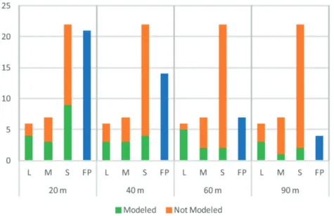
Because of this divergence in the performances we decided to carry out an additional test by comparing modelled overdeepenings and existing lakes for the four runs (Fig. 11). We notice that the 20 m run has the highest number of modelled lakes but it is also the one with the highest number of false positive. Most of them are located at glacier margins where the calculation of glacier surface slopes could be uncer-tain and consequently results in artefacts. Modelled lakes as well as false positive decrease with the decrease of the spatial resolution. Looking at the largest modelled lakes, we note that all the four runs modelled about more than the 50% of the large lakes (N10,000 m2).
The 60 m run gives the best performance among the four runs in modelling large lakes (5 of the 6 lakes modelled). The 20 and 40 m ver-sions perform better than the 60 m run for small lakes and similarly to 60 m run for medium lakes but false positive are the triple and the dou-ble in the 20 m and 40 m versions respectively if compared to the 60 m. The 90 m run performs worst except for the small number of false positives.
We decided to focus on the results of the 60 m run in the present work because of: 1) good performance in modelling the largest lakes, potentially the most dangerous; 2) few false positive; 3) correct
Fig. 5. Comparison between modelled bedrock and real surface (2008 LIDAR DTM) for two cases (a, Mont Gelé Glacier and b, Invergnan Glacier) where an overdeepening has been modelled but no real lake exists.
(Imagery: Italian National Geoportal. 2006–07 orthophotos.)
Fig. 6. Maps of the modelled bedrock elevation (elevation contours) and ice thickness (grey scale grid) at a) Gran Etret (top left) and b) Indren (bottom right) glaciers. The interval of the elevation contours is 30 m a.s.l. Plots show the cross-sectional and longitudinal profiles modelled with GlabTop2 and the model uncertainty of ±30%, the GPR measurements and the GPR uncertainty.
calculation of small lakes is not demanded in the present study (consid-ering the limited ability of the model to reproduce small-scale features).
5. Discussion
5.1. Future landscape evolution
Within the study area, the volume of calculated potential overdeepenings (0.06 km3) is only 0.8% of the corresponding total glacier volume (7.3 km3 in 1991). Considering similar studies implementing the GlabTop approach, we notice that the calculated value is less than the corresponding one for the Swiss Alps (3%,
Linsbauer et al., 2012) and the Himalaya-Karakoram (3–4%,Linsbauer et al., 2016). However, similar values (0.5, 1%) were found for the Peruvian Andes (Colonia et al., 2017). Considering thatflat areas (like
valley glacier tongues) are more suitable for the modelling of overdeepenings, the higher value for the Swiss Alps can be due to the fact that the results refer to 1973 when glaciers were wider andflat tongues still existed. For the Himalaya-Karakoram the input datasets are more recent (2000–2010) and, accordingly toBolch et al. (2012), at that stage a large part of the ice in the region was still located in the flat tongues of the valley glaciers. Finally, similarity with the study of
Colonia et al. (2017)in the Peruvian Andes can be due to the limited ex-tent of remainingflat glacier parts. Many Peruvian glaciers, similar to the glaciers of the Aosta Valley, lost theirflat and thick tongues, where lakes could form, in the recent past.
In Aosta Valley Region, the surface area occupied by lakes (1.1 km2) corresponds to about 0.6% of the area exposed through glacier retreat (179 km2) over the time period (1850–1991). The total area of modelled overdeepenings (3.1 km2) corresponds to 1.9% of the remain-ing glacier area in 1991 (163 km2). The differences in the values could be attributed to the fact that not all the past overdeepenings arefilled with water, originating a lake. The same can happen in the future, espe-cially considering the increase in the amount of debris in glacier basins becoming exposed on slopes, which will likely fill some of the overdeepenings once they become exposed by glacier retreat. The mation of breaches in dams at overdeepenings can also prevent lake for-mation, as discussed byColonia et al. (2017).
More than a half of the potential overdeepenings are located in the lowest areas of the glaciers and they correspond to the smallest and shallowest elements of the population. The glaciers will probably free the areas where these overdeepenings are located in the coming years. The largest and deepest overdeepenings are located in the accu-mulation areas of the widest and thickest glaciers of the region (Tribolazione, Rutor, Pre de Bar, Triolet, Grandes Murailles), located in the highest mountain massifs. According to future scenarios, these larg-est glaciers will probably survive in the coming decades becoming
Fig. 7. Radargram of the corresponding longitudinal GPR profile AA′ at Indren Glacier.
Fig. 8. Maps of the two overdeepenings modelled in the lower (L) and upper (U) zone of the Rutor Glacier, corresponding ice thickness and location of GPR paths (a). Plots show the cross-sectional profiles (ll′ in b and uu′ in c) modelled with GlabTop2 and the model uncertainty of ±30%, the GPR measurements and the GPR uncertainty.
(Imagery: Italian National Geoportal. 2006–07 orthophotos.)
increasingly important with their ice reserves (Zemp et al., 2006;
Linsbauer et al., 2012; Zekollari et al., 2019). Hence, the related overdeepenings will not appear very soon but nevertheless probably before the end of the century.
5.2. Model performance
Similarly to other authors (Farinotti et al., 2017), in the present study we demonstrated that models inferring ice thickness from surface to-pography are limited in their ability to reproduce small-scale features of bed topography. However, it should be stated that an accurate simu-lation of very small glacier lakes is not a crucial demand, because they rarely constitute a hazard or cause relevant issues for environmental management.
A qualitative comparison between modelled overdeepenings and existing lakes shows a good performance of GlabTop2 in terms of location of modelled overdeepenings and lakes, especially for the lakes with area larger than 10,000 m2(Fig. 12a, b, c). The model is also able to predict the location of some of the medium size lakes (area between 5000 and 10,000 m2) as shown inFig. 12d.
Regarding false negatives, we note that the majority of them are lo-cated in steep areas (slope N 20°) of small glaciers (surface area b 1 km2). On such glaciers ice thickness in the centre is not much thicker than at the margin, which is a possible reason for this type of“error”. Furthermore, and as mentioned above, the model has limited abilities to reproduce small-scale landforms (N70% of the false negatives are small lakes, areab 5000 m2).
Fig. 9. Scatter plot of mean depth of modelled overdeepenings versus their area as modelled for the 20 m, 40 m, 60 m and 90 m runs. The table (top left) reports the main morphometric parameters of the overdeepenings for the four different spatial resolutions.
Fig. 10. Comparison between outputs of glacier bed model using DEMs sampled to 60 m and 20 m and GPR measurements along cross-sections at the Gran Etret and Indren Glacier.
Fig. 11. Model performances for the four different runs (20 m, 40 m, 60 m and 90 m); for each run the number of modelled (green) and not modelled (red) real lakes are given, differentiating among large (L, areaN 10,000 m2
), medium (M, area between 5000 and 10,000 m2
) and small (S, areab 5000 m2
) existing lakes and the overdeepenings that do not correspond to real lakes (blue, false positive, FP).
Only two of the seven false positives are clearly artefacts (ID 13 and ID 14 inTable 2andFig. 12e and f). From a geomorphological point of view, they correspond to areas not characterized by a bedrock overdeepening in the real-world, the slope is uniform. They are gener-ated where the glacier surface in the year 1991 was of shallow slope (about 11°), thus likely to result in modelled overdeepenings. However, they are also located very close to the glacier margins where the model often tends to create spurious overdeepenings. The remaining false pos-itives could be real overdeepenings but they are nowadaysfilled by sed-iment or dead ice instead of water (e.g.: ID 15,Fig. 5a). In one case water ponds are currently forming (ID 16,Fig. 5b).
An exception is the Rutor Glacier (Fig. 12a) whose proglacial area features two modelled overdeepenings (ID 2 and ID 5) that are located in the vicinity, but do not overlap, with two current lakes (M and L2). This result can be interpreted as an ability of the model to identify, at least, areas prone to lakes formation.
We also compared the location of the modelled overdeepenings with morphological criteria described byFrey et al., 2010a(Fig. 13a) to identify potential locations of overdeepenings. The reported
examples (Fig. 13b, c) show a good correspondence with the three criteria: 1) distinct break in slope; 2) reduction in glacier width; 3) heavily crevassed glacier part below a crevasse-free part. The location of modelled overdeepenings also correspond well with areas with sur-face slopeb 5°, as a first-order criterion for pre-selecting sites with pos-sible overdeepenings (Frey et al., 2010a). We can confirm that the location of the modelled overdeepenings is quite robust while other pa-rameters, like size and depth, are less certain.
Some issues in modelling ice thickness and consequently overdeepenings are noticed in theflat and wide areas of the glaciers, as demonstrated in the case of Rutor Glacier (Fig. 8). In such areas, the model might overestimate actual ice thickness. In fact, the Rutor Glacier cannot be defined as a typical valley or mountain glacier, and probably its dynamic is highly influenced by the structural lineaments of the bedrock: these could be the reasons of such divergence between measured and modelled values. In addition, the upperflat (firn) zone is close to a“firn divide” where surface slope becomes zero and the basic assumption of the GlabTop approach (constant basal shear stress) is no longer valid. The differences between GPR data and model results
Fig. 12. Comparison between the location of modelled overdeepenings (green outlines) and existing large (L) and medium (M) lakes within 1991 glacier extents (black lines) in the study area (a, b, c, d). Panels e and f show examples of model artefacts (false positive).
(Imagery: Italian National Geoportal. 2012 orthophotos.)
remain unresolved, especially for the site in the lower zone which fulfils all conditions for the formation of an overdeepening according toFrey et al. (2010a). Potential inaccuracies during the acquisition and inter-pretation of the GPR data have also to be taken into account. In fact, the accuracy in estimating the depth of the interface between ice and bedrock is challenging and depends on several factors such as: mor-phology of the radiated surface; dielectric permittivity of the ice and its thickness; tilt-angle of the radiation with respect to the inclination of the target; frequency of the radar signal; scattering phenomena due to the presence of heterogeneities in the ice; wave velocity of the ice de-pending on the ice density. Because of these challenges in the GPR data acquisition and interpretation, they should always be used with care when validating modelled bed topography.
5.3. Backward and forward validation
We believe that the backward approach represents a solid way for validating and evaluating the performance of the model. In particular, the backward approach allows comparing modelled results with real lakes and topography of deglaciated areas. In comparison, GPR data often used for validation (e.g.Farinotti et al., 2017;Frey et al., 2014) can be subjected to large uncertainties because of challenging data ac-quisition and interpretation (Colonia et al., 2017).
Extensive GPR coverage is needed for a good comparison of measured and modelled bedrock because of the large pixel size of the output raster. Short GPR tracks can be used for the validation of the ice thickness at some specific points but they cannot validate the general shape of the bedrock and, in the case of identification of overdeepenings, their real ex-istence. Moreover, analysing typically linear GPR profiles is challenging because an overdeepening is only fully defined in three dimensions, and the multiple 3D radar reflections imply uncertainties in interpretation. For these reasons, in a GPR survey planning it is necessary to consider the glacier size and shape and the GPR tracks must be long enough in both longitudinal and transversal directions.
5.4. Effect of the input data on model results
The spatial resolution of the input DEM influences modelled ice thickness. The smaller the pixel size, the higher the ice thickness, the larger the number of modelled overdeepenings but also the higher the number of false positives. Moreover, as suggested byPaterson (1994)
andHaeberli and Hoelzle (1995), the relationship between surface
slope and ice thickness is strongest along the centralflowline of a glacier and breaks down towards the margins (both laterally and near glacier top and terminus). These issues have to be taken into account in the future implementation of GlabTop2.
The comparison between measured and modelled bedrock profiles shows that the morphological variability of the glacier surface (repre-sented by the DEM) is transferred to the modelled bedrock topography because it is calculated by subtraction of modelled ice thickness from the DEM (Paul and Linsbauer, 2012). This explains the better perfor-mances, in terms of qualitative agreement, for the high spatial resolu-tion run. Comparing existing lakes with the modelled overdeepenings of the four runs, we found that larger lakes have been well modelled, which confirms the robustness of the model in assessing the location of the overdeepenings and approximately their size.
Based on our results, we recommend to choose a medium pixel size (about 60 m) to avoid a great number of false positive and overestima-tion of ice thickness, number of overdeepenings, depth and volume.
6. Conclusions
The results of the application of the GlabTop2 model to the glaciers of the Aosta Valley Region quantify newest ice volumes for the largest glacierized region of Italy (5.2 ± 1.6 km3of total glacier volumes) and the location of potential future glacier lakes (46 potential future overdeepenings covering a total area of 3.1 ± 0.9 km2). Future lake models were missing so far for Italy: therefore, this studyfills an impor-tant research gap by modelling glacial bed overdeepenings and potential future lakes for the Aosta Valley, the region with the most extensive gla-cier cover in Italy. Application of this information can be important for the management of water resources and risks related to glacier lakes.
The volume of modelled potential future overdeepenings represents only 0.8% of the total modelled glacier volume. We estimate that, con-tinued glacier retreat, will expose mainly smaller and shallower overdeepenings. Larger and deeper geomorphological troughs will re-mainfilled by ice for a few more decades.
In addition to the use of well-known methodologies for validation of model of ice thickness and overdeepenings (GPR surveys and morpho-logical criteria), we have proposed a further approach termed “back-ward approach” that has proven to be useful to compare modelled glacier-bed overdeepenings and real-world landforms. Obviously, GPR surveys remain essential to detect not already exposed overdeepenings
Fig. 13. Morphological criteria fromFrey et al. (2010a)(a) that indicate the potential existence of glacier-bed overdeepenings for two cases in the study area: Pre de Bar Glacier (b, Mont Blanc Massif) and Coupé de Money Glacier (c, Gran Paradiso Chain).
(Imagery: Italian National Geoportal. 2006–07 orthophotos.)
but always considering the challenges in the GPR data acquisition and interpretation.
Considering the GlabTop approach, we have found that the location of the modelled overdeepenings is robust while a higher level of uncer-tainty remains in the dimensions of the overdeepenings.
Combining the analysis of the location of modelled lakes with glacier retreat scenarios will allow to define the approximate year or decade during which the potential lakes will appear.
To our knowledge, overdeepenings underneath Italian glaciers have not yet been modelled. Extending the modelling to the rest of the Italian Alps would be important for estimating the total amount of water stored in the future lakes and for understanding how the alpine envi-ronment will look in the future, following continued glacier shrinkage.
Declaration of competing interest
The authors declare that they have no known competingfinancial interests or personal relationships that could have appeared to in flu-ence the work reported in this paper.
Acknowledgments
The authors acknowledge Umberto Morra di Cella (ARPA Valle d'Aosta) for sharing GPR data of the Gran Etret Glacier and Andrea Tamburini and Fabio Villa (IMAGEO S.r.l.) for those of the Rutor Glacier. Moreover, a special thanks to Nicola Colombo and Arnoldo Welf for their technical support in the GPR survey at Indren Glacier in September 2016. The authors are furthermore grateful towards the two anony-mous reviewers and Holger Frey for constructive reviews that substan-tially improved the manuscript.
This research did not receive any specific grant from funding agen-cies in the public, commercial, or not-for-profit sectors.
References
Ajassa, R., Biancotti, A., Biasini, A., Brancucci, G., Caputo, C., Pugliese, F., Salvatore, M.C., 1994. Il catasto dei ghiacciai italiani: primo confronto tra i dati 1958 e 1989. Il Quaternario 7 (1), 497–502. http://www.aiqua.it/en/index.php/volume-7-1-b/782-il-catasto-dei-ghiacciai-italiani-primo-confronto-tra-i-dati-1958-e-1989/file. Ajassa, R., Biancotti, A., Biasini, A., Brancussi, G., Carton, A., Salvatore, M.C., 1997. Changes
in the number and area of Italian Alpine glaciers between 1958 and 1989. Geogr. Fis. Din. Quat. 20, 293–297.http://www.glaciologia.it/wp-content/uploads/FullText/full_ text_20_2/16_GFDQ_20_2_Ajassa_293_297.pdf.
Allen, S.K., Schneider, D., Owens, I.F., 2009. First approaches towards modelling glacial hazards in the Mount Cook region of New Zealand’s Southern Alps. Nat. Hazards Earth Syst. Sci. 9, 481–499.https://doi.org/10.5194/nhess-9-481-2009.
Bolch, T., Buchroithner, M.F., Peters, J., Baessler, M., Bajracharya, S., 2008. Identification of glacier motion and potentially dangerous glacial lakes in the Mt. Everest region/Nepal using spaceborne imagery. Nat. Hazards Earth Syst. Sci. 8, 1329–1340.https://doi.org/ 10.5194/nhess-8-1329-2008.
Bolch, T., Peters, J., Yegorov, A., Pradhan, B., Buchroithner, M., Blagoveschchensky, V., 2011. Identification of potentially dangerous glacial lakes in the northern Tien Shan. Nat. Hazards 59 (3), 1691–1714. https://doi.org/10.1007/s11069-011-9860-2.
Bolch, T., Kulkarni, A., Kääb, A., Huggel, C., Paul, F., Cogley, J.G., Frey, H., Kargel, J.S., Fujita, K., Scheel, M., Bajracharya, S., Stoffel, M., 2012. The state and fate of Himalayan gla-ciers. Science 336 (6079), 310–314.https://doi.org/10.1126/science.1215828. Buckel, J., Otto, J.C., Prasicek, G., Keuschnig, M., 2018. Glacial lakes in Austria - distribution
and formation since the Little Ice Age. Glob. Planet. Chang. 164, 39–51.https://doi. org/10.1016/j.gloplacha.2018.03.003.
Capps, D.M., Clague, J.J., 2014. Evolution of glacier-dammed lakes through space and time; Brady Glacier, Alaska, USA. Geomorphology 210, 59–70.https://doi.org/10.1016/j. geomorph.2013.12.018.
Carrivick, J.L., Tweed, F.S., 2013. Proglacial lakes: character, behavior and geological im-portance. Quat. Sci. Rev. 78, 34–52.https://doi.org/10.1016/j.quascirev.2013.07.028. CGI-CNR– Comitato Glaciologico Italiano & Consiglio Nazionale delle Ricerche, 1961.
Catasto dei Ghiacciai Italiani, Anno Geofisico Internazionale 1957–1958. Ghiacciai del Piemonte. 2. Comitato Glaciologico Italiano, Torino (324 pp.).
Čiamporová-Zaťovičová, Z., Čiampor, F., 2017. Alpine lakes and ponds - a promising source of high genetic diversity in metapopulations of aquatic insects. Inland Waters 7 (1), 109–117.https://doi.org/10.1080/20442041.2017.1294361.
Citterio, M., Diolaiuti, G.A., Smiraglia, C., D’Agata, C., Carnielli, T., Stella, G., Siletto, G.B., 2007. Thefluctuations of Italian glaciers during the last century: a contribution to knowledge about alpine glacier changes. Geogr. Ann. A 89 (3), 164–1821.https:// doi.org/10.1111/j.1468-0459.2007.00316.x.
Colonia, D., Torres, J., Haeberli, W., Schauwecker, S., Braendle, E., GIraldez, C., Cochachin, A., 2017. Compiling an inventory of glacier-bed overdeepenings and potential new lakes in de-glaciating areas of the Peruvian Andes: approach,first results, and per-spectives for adaptation to climate change. Water 9 (5), 336.https://doi.org/ 10.3390/w9050336.
Diolaiuti, G., Smiraglia, C., 2010. Changing glaciers in a changing climate: how vanishing geomorphosites have been driving deep changes in mountain landscapes and environ-ments. Géomorphologie 16 (2), 131–152.https://doi.org/10.4000/geomorphologie.7882. Diolaiuti, G.A., Citterio, M., Carnielli, T., D’agata, C., Kirkbride, M., Smiraglia, C., 2006. Rates,
processes and morphology of fresh-water calving at Miage Glacier (Italian Alps). Hydrol. Process. 20, 2233–2244.https://doi.org/10.1002/hyp.6198.
Diolaiuti, G.A., Bocchiola, D., Vagliasindi, M., D’Agata, C., Smiraglia, C., 2012. The 1975–2005 glacier changes in Aosta Valley (Italy) and the relations with climate evolution. Prog. Phys. Geogr. 36 (6), 764–785.https://doi.org/10.1177/0309133312456413.
Drenkhan, F., Guardamino, L., Huggel, C., Frey, H., 2018. Current and future glacier and lake assessment in the deglaciating Vilcanota-Urubamba basin, Peruvian Andes. Glob. Planet. Chang. 169, 105–118.https://doi.org/10.1016/j.gloplacha.2018.07.005. Drenkhan, F., Huggel, C., Guardamino, L., Haeberli, W., 2019. Managing risks and future
options from new lakes in the deglaciating Andes of Peru: the example of the Vilcanota-Urubamba basin. Sci. Total Environ. 665, 465–483. https://doi.org/ 10.1016/j.scitotenv.2019.02.070.
Dutto, F., Mortara, G., 1992. Rischi connessi con la dinamica glaciale nelle Alpi Italiane. Geogr. Fis. Din. Quat. 15, 85–99.http://www.glaciologia.it/wp-content/uploads/ FullText/full_text_15_1_2/11_GFDQ_15_1_2_Dutto_85_99.pdf.
Emmer, A., Vilímek, V., Klimeš, J., Cochachin, A., 2014. Glacier retreat, lakes development and associated natural hazards in Cordilera Blanca, Peru. In: Shan, W., Guo, Y., Wang, F., Marui, H., Strom, A. (Eds.), Landslides in Cold Regions in the Context of Climate Change. Environmental Science and Engineering. Springer, Cham, pp. 231–252
https://doi.org/10.1007/978-3-319-00867-7_17.
Emmer, A., Merkl, S., Mergili, M., 2015. Spatiotemporal patterns of high-mountain lakes and related hazards in western Austria. Geomorphology 246, 602–616.https://doi. org/10.1016/j.geomorph.2015.06.032.
Emmer, A., Klimeš, J., Mergili, M., Vilímek, V., Cochachin, A., 2016. 822 lakes of the Cordil-lera Blanca: an inventory, classification, evolution and assessment of susceptibility to outburstfloods. Catena 147, 269–279.https://doi.org/10.1016/j.catena.2016.07.032. Farinotti, D., Huss, M., Bauder, A., Funk, M., Truffer, M., 2009. A method to estimate the ice
volume and ice-thickness distribution of alpine glaciers. J. Glaciol. 55 (191), 422–430.
https://doi.org/10.3189/002214309788816759.
Farinotti, D., Brinkerhoff, D.J., Clarke, G.K.C., Fürst, J.J., Frey, H., Gantayat, P., Gillet-Chaulet, F., Girard, C., Huss, M., Leclercq, P.W., Linsbauer, A., Machguth, H., Martin, C., Maussion, F., Morlighem, M., Mosbeux, C., Pandit, A., Portmann, A., Rabatel, A., Ramsankaran, R., Reerink, T.J., Sanchez, O., Stentoft, P.A., Singh Kumari, S., van Pelt, W.J.J., Anderson, B., Benham, T., Binder, D., Dowdeswell, J.A., Fischer, A., Helfricht, K., Kutuzov, S., Lavrentiev, I., McNabb, R., Gudmundsson, G.H., Li, H., Andreassen, L.M., 2017. How accurate are estimates of glacier ice thickness? Results from ITMIX, the Ice Thickness Models Intercomparison eXperiment. Cryosphere 11, 949–970.
https://doi.org/10.5194/tc-11-949-2017.
Fischer, U.H., Haeberli, W., 2012. Overdeepenings in glacial systems: processes and uncer-tainties. Eos 93 (35), 341.https://doi.org/10.1029/2012EO350010.
FMS– Fondazione Montagna Sicura, 2016. Bilancio sociale e di Missione 2016. 68 pp.http:// www.fondazionemontagnasicura.org/eventi/bilancio-sociale-e-di-missione-2016. Frey, H., Haeberli, W., Linsbauer, A., Huggel, C., Paul, F., 2010a. A multi-level strategy for
anticipating future glacier lake formation and associated hazard potential. Nat. Haz-ard. Earth Sys. 10, 339–352.https://doi.org/10.5194/nhess-10-339-2010.
Frey, H., Huggel, C., Paul, F., Haeberli, W., 2010b.Automated detection of glacier lakes based on remote sensing in view of assessing associated hazard potentials. In: Kaufmann, V., Sulzer, W. (Eds.), Proceedings of the 10th International Symposium on High Mountain Remote Sensing Cartography. Grazer Schriften der Geographie und Raumfoschung 45, pp. 261–272.
Frey, H., Machguth, H., Huss, M., Huggel, C., Bajracharya, S., Bolch, T., Kulkarni, A., Linsbauer, A., Salzmann, N., Stoffel, M., 2014. Estimating the volume of glaciers in the Himalayan–Karakoram region using different methods. Cryosphere 8, 2313–2333.https://doi.org/10.5194/tc-8-2313-2014.
Galluccio, A., 1998. I nuovi laghi proglaciali lombardi. Terra glacialis 1, 133–151.http:// lnx.servizioglaciologicolombardo.it/index.php/pubblicazioni/terra-glacialis/347-01-terra-glacialis-nd-1.
Gardelle, J., Arnaud, Y., Berthier, E., 2011. Contrasted evolution of glacial lakes along the Hindu Kush Himalaya mountain range between 1990 and 2009. Glob. Planet. Chang. 75 (1–2), 47–55.https://doi.org/10.1016/j.gloplacha.2010.10.003. Giardino, M., Mortara, G., Chiarle, M., 2017. The glaciers of the Valle d’Aosta and Piemonte
regions: records of present and past environmental and climate change. In: Soldati, M., Marchetti, M. (Eds.), Landscapes and Landforms of Italy. World Geomorphological Landscapes. Springer, Cham, pp. 77–88https://doi.org/10.1007/978-3-319-26194-2_6. Haeberli, W., Hoelzle, M., 1995. Application of inventory data for estimating
characteris-tics of and regional climate-change effects on mountain glaciers: a pilot study with the European Alps. Ann. Glaciol. 21, 206–212. https://doi.org/10.3189/ S0260305500015834.
Haeberli, W., Buetler, M., Huggel, C., Lehmann Friedli, T., Schaub, Y., Schleiss, A.J., 2016a. New lakes in deglaciating high-mountain regions– opportunities and risks. Clim. Chang. 139 (2), 202–214.https://doi.org/10.1007/s10584-016-1771-5.
Haeberli, W., Linsbauer, A., Cochachin, A., Salazar, C., Fischer, U.H., 2016b. On the morpho-logical characteristics of overdeepenings in high-mountain glacier beds. Earth Surf. Process. Landf. 41, 1980–1990.https://doi.org/10.1002/esp.3966.
Hanshaw, M.N., Bookhagen, B., 2014. Glacial areas, lake areas, and snow lines from 1975 to 2012: status of the Cordillera Vilcanota, including the Quelccaya Ice Cap, northern central Andes, Peru. Cryosphere 8, 359–376.https://doi.org/10.5194/tc-8-359-2014.