Essays on financial markets predictability

(1)

Essays on Financial Markets

Predictability

A dissertation presented by

Matteo Maria Pisati

Supervised by

Professor Giovanni Barone-Adesi

(Main Advisor) and

Professor Antonietta Mira

(Co-Advisor)

Submitted to the

Faculty of Economics

Universita’ della Svizzera italiana

for the degree of

(2)

(3)

Acknowledgements

I am very grateful to my advisors Professor Giovanni Barone-Adesi and Professor Antonietta Mira, for their very patient guidance and trust, from my early SNF research proposal through to completion of this degree. I would never be able to complete this work without their continuous support.

I also wish to express my gratitude toward the Swiss National Foundation (SNF) for the funding of the project number 100018 172892 (”Market Predictabil-ity and its Rationale: new insights in the theoretical and empirical analysis of the pricing kernel”). Without their generosity this thesis would have never been finished.

Finally, a deep thanks to my parents Gianni and Laura, to whom this work is dedicated, for their constant support and encouragement through all my life.

(4)

Chapter 1 Introduction

The current study is all about the elusive nature of market predictability. This topic has captured huge attention because of its intrinsic economic value and be-cause it is intimately related to financial theory. Indeed, accordingly, to the neo-classical theory of finance market are unpredictable beyond the risk premia. Still, in recent years, the efficient market hypothesis and the related random-walk as-sumption of financial markets felt under rising pressure, and evidence is mounting that financial markets are far from being completely efficient. This new evidence is closely linked with the recent spur in the field of artificial intelligence and a more mature understanding of the behavioral dynamics of financial markets.

The first part of this work involves the study of the famous sentiment index

proposed by Baker and Wurgler [2006] (B-W from now on). Indeed, while a big

literature proposes alternative measures of sentiment, we still lack a precise un-derstanding of what ultimately sentiment is. The empirical analyses performed show how the B-W sentiment index is effective only in detecting situations of abnormally low levels of risk pricing but fails in detecting abnormally high lev-els of risk pricing consequently the B-W index can be better understood as an index of greed. Interestingly, the results show how the B-W sentiment index is tightly linked with uncertainty (defined as the dispersion in investors’ views) and is Granger caused by the changes in the most optimistic views in the investors’ spectrum. These results point in favor of an understanding of financial markets in which during bull markets, prices are driven by the most optimistic (less risk-averse) investors. Furthermore, our results point in favor of an understanding of financial markets in which a dichotomy exists between the asset prices estimated by the representative investor, which reflects the investors value-weighted average views, and market asset prices (marginal investor prices in the text), which re-flect the investors constrained value-weighted average among all investors views. Indeed, in the real world investors are constrained by many legal and regulatory

(7)

constraints that deter them from implementing their views. The dichotomy holds in equity markets and explains why the B-W index, which is extrapolated from equity-based measures, can detect only abnormally low levels of risk pricing. Af-ter that, we propose a fear proxy, which is complementary in Af-terms of time series and cross-sectional predictive power to the B-W index. Our measure is indeed effective in detecting abnormally high levels of risk pricing only. Our measure of fear is based on a measure of illiquidity and skewness coming from the risk-neutral distribution extrapolated from options. Indeed, options markets are largely driven by hedging needs and are intrinsically forward-looking and consequently are well suited to detect abnormally high levels of risk aversion. Importantly, our results hold well in forecasting the S&P 500, both in-sample and out-of-sample. Subse-quently, we find that our fear measure is specular to the B-W sentiment index even at the cross-sectional level completing with the ability to time the short leg

of the anomalies the results ofStambaugh et al.[2012] which proved how the B-W

sentiment index was effective in timing the long leg of the anomalies. Finally, the results found at the cross-sectional level shows how conditionally on a high level of fear the expected return per unit of risk is higher than on average while the opposite holds for the B-W sentiment proxy.

The second part of this research studies the three key ingredients of out-of-sample predictability: predictive models, predictors, and the function of market uncertainty that we aim at predicting. At first, we merge machine learning and model selection approaches to achieve superior predictive accuracy using as

in-puts the well-known predictors of Welch and Goyal [2008]. The results show how

combining more and more powerful predictive approaches is possible to raise the predictive accuracy out-of-sample for the returns of the S&P 500 and that our re-sults hold even for the most recent years. After that, we employ as predictors the

spread returns of the eleven anomalies employed by Stambaugh et al. [2012], and

we observe how these predictors exhibit a record high predictive power in terms of

R2

OS and ∆ Utility with regards to the S&P 500 even when employed in univariate

linear regressions. Finally, the approach proposed by Bakshi and Madan [2000]

is studied under the lenses of out-of-sample predictability. Our results show how

the returns of the moments’ contracts introduced by Bakshi and Madan [2000],

which are built through a linear combination of call and put options, exhibit R2_OS

and ∆ Utility values well above the ones traditionally recorded for the S&P 500.

Consequently, given the flexibility of the approach proposed byBakshi and Madan

[2000] it becomes possible to synthesize new securities with highly predictable

re-turns revering the traditional issue of market predictability: instead of working on highly sophisticated models to predict hard to forecast securities, it becomes possible to create and trade new complex securities which are easier to forecast.

(8)

The third part of this work studies the dynamics of predictability itself. The

starting point is the understanding that the time series of the R2

OS coming from

different models and-or predictors can provide a valuable source of information on the genesis of predictability. After that, the analyses focus on understanding whether predictability stems from changes in economic fundamentals or investors’ sentiment. From a theoretical point of view, this study is linked to the ongoing debate between behavioral and neoclassical finance. Indeed, the theory on asset pricing is divided into two main conflicting schools of thought: the neoclassical approach, which states that higher expected returns are a consequence of higher risks and the behavioral approach, which explains how human biases lead investors to deviate from full rationality. Empirical results show how the interaction among risks and the pricing of risks is at the very base of predictability, and consequently, both behavioral and neoclassical theories provide useful tools in understanding fi-nancial markets. After that, our results combined suggest how different typologies of market predictors have a changing predictive power accordingly to the prevail-ing market regime. More in detail, fundamentals are the main drivers and are more precisely incorporated into prices during bear markets, while during bullish markets, the dynamics of risk pricing are more relevant, and non-fundamental (technical, trend following, behavioral) signals have a higher impact. Finally, we study the causality dynamics among behavioral and fundamentals variables, and we document how, on average, are changes in fundamentals (risks) that trigger changes in behavioral variables (risk premia). These relations are stronger (in terms of magnitude, statistical power, and the number of statistically significant predictors) during the bear than during the bull regime. This helps to explain the dominant role played by fundamentals in forecasting market returns during

recessions. Our results reject the theory advanced by Julien and Michael [2017],

who explains the higher probability detected during economic recessions through the existence of an uncertainty risk premium. Indeed, all our analyses confirm how the level of uncertainty has no explanatory power for predictability dynamics in bear markets. In bull markets, on the other hand, the impact of fundamen-tals is weaker, and the dynamics of uncertainty, which drive risk premia, have a larger impact in explaining predictability. From a theoretical perspective the

habit theory introduced byCampbell and Cochrane [1999], which explains market

time-varying risk premia through a utility function which discounts more risks in bad than in good times, is largely consistent with our empirical evidence: prices are driven by changes in current fundamentals (risks) which trigger changes in behavioral variables (risks pricing).

(9)

Bibliography

Baker, M. and Wurgler, J. (2006). Investor sentiment and the cross-section of stock returns. The Journal of Finance, 61(4):1645–1680.

Bakshi, G. and Madan, D. (2000). Spanning and derivative-security valuation. Journal of Financial Economics, 55(2):205–238.

Campbell, J. Y. and Cochrane, J. H. (1999). By force of habit: A consumption-based explanation of aggregate stock market behavior. Journal of Political Econ-omy, 107(2):205–251.

Julien, C. and Michael, H. (2017). Why does return predictability concentrate in bad times? The Journal of Finance, 72(6):2717–2758.

Stambaugh, R. F., Yu, J., and Yuan, Y. (2012). The short of it: Investor sentiment and anomalies. Journal of Financial Economics, 104(2):288 – 302. Special Issue on Investor Sentiment.

Welch, I. and Goyal, A. (2008). A comprehensive look at the empirical performance of equity premium prediction. The Review of Financial Studies, 21(4):1455– 1508.

(10)

Chapter 2 Greed and Fear

2.1 Introduction

In the last decade, financial economists have devoted huge efforts to study the impact of sentiment on financial markets. Surprisingly, while an extensive list of

studies employs sentiment proxies1_{, it is still not clear what sentiment really is.}

With this study, we aim at providing an empirically based answer. To achieve it, we explore the links among uncertainty, sentiment, and fear. These findings allow us to reconcile, inside a unified framework, the puzzling evidence coming from the

research on options2 and on the relative underlying stocks3.

We build on the existing literature on uncertainty4 _{to understand the main drivers}

of sentiment and fear. The empirical evidence emerging from our analysis suggests that the currently employed proxies for sentiment are driven by both uncertainty and the most optimistic investors while the proxies for fear are driven by uncer-tainty and the most pessimist views. Our results show that sentiment and fear proxies are complementary in their out of sample predictive ability, with sentiment (fear) indexes especially powerful in predicting negative (positive) returns. Con-sequently, these indexes are effective in detecting abnormally low (sentiment) or high (fear) levels of risk aversion but not both of them jointly. After that, we show how conditioning on the presence or absence of high levels of fear or sentiment

1_{See, e.g.,} _{Baker and Wurgler}_[₂₀₀₆_];_{Baker et al.} _[₂₀₁₂_];_{Stambaugh et al.}_[₂₀₁₂_]; _{Israel and}

Moskowitz[2013]

2_{Andersen et al.}_[₂₀₁₅_{] and}_{Bollerslev et al.}_[₂₀₁₅_{] show how factors driving the left tail of the}

risk-neutral distribution can predict the market while the same does not apply for the factors coming from the right tail

3_{The impact of sentiment and fear on cross-sectional returns has been recently addressed by}

Stambaugh et al.[2015], andFarago and T´edongap[2018]

4_{Among the studies which influenced our subsequent analysis we especially highlight}_Diether

(11)

the out-of-sample predictability and the risk-return relation for the most relevant anomalies detected in the empirical literature varies dramatically. Depending on the prevailing market conditions, we observe subsequent high or low return per unit of risk. Consequently, we prove how the same indicators which are complementary in timing the aggregate market are even complementary in timing the anomalies: a unique logic drive returns both at a market wide and at a cross-sectional level.

The empirical analysis makes use of an extensive amount of indexes of uncertainty5

and fear6 _{coming from the existing literature and it is further augmented by newly}

proposed indexes of fear following Barone-Adesi et al. [2008] and Barone-Adesi

[2016]. This paper enrich the existing literature building simple, yet powerful,

measures of fear coming from the left tail and the skewness of the option risk-neutral distribution. These measures exploit the forward-looking nature of op-tions to detect abnormally high levels of risk aversion (fear). We show how the differences between option implied percentiles have a remarkable predictive power out-of-sample. To the best of our knowledge, this is the first study that makes use of option implied information to time cross-sectional returns (the so-called ‘anomalies’) both in sample and out of sample.

Acting as one of the main driver of the paper, we introduce the conceptual di-chotomy between the marginal and the representative investor which provides a theoretical rationale for our empirical analysis. Prices reflect the views of the opti-mistic investors (the marginal ones) and these views can diverge from mean views (the representative investor’s ones). The divergence occurs because in many cases legal and regulatory constraints do not allow for short selling. Consequently, from stocks, it is only possible to infer proxies that detect excessive low risk aversion (overbought or greed) while options are needed to infer the complementary mea-sures which detect excessive high risk aversion (oversold). On the ground of the stated dichotomy, this work addresses inside a coherent framework, some of the issues that are still left open by the previous literature.

The first issue concerns the relationship between sentiment and uncertainty. In

their work Stambaugh et al. [2012] do not assign a role for a time varying

cross-sectional dispersion of views. They simply hypothesize that the views of the most optimistic investors in the cross-section are more likely to be too optimistic when the measure of investor sentiment is high than when it is low. That can occur for different reasons. As the sentiment measure rises, the cross-sectional mean of investors views can remain near to a reasonable valuation level while the cross-sectional dispersion of views increases. Alternatively, as the sentiment measure

5_{E.g. the analysits dispersion of the views of}_Yu_[₂₀₁₁_{] and the macroeconomic and financial}

uncertainty indexes of Jurado et al.[2015]. See the section 2 on Data for the full list

6_{E.g. the VIX index, the Variance Risk Premium, the Crash Confidence Index, the tail}

measure ofBollerslev et al.[2015], the pricing kernel tail measure of Almeida et al.[2017]. See

(12)

increases, the dispersion of opinions can remain relatively constant, or even fall, while the mean of investors views increases significantly above a rational valuation level. This paper addresses this critical dilemma, and analyzes the link between uncertainty and sentiment. In our empirical analysis, we show how sentiment and uncertainty are closely linked and how sentiment is driven by the most optimist views which are Granger caused by uncertainty.

The second issue comes from Andersen et al. [2015]. The authors find that the

left tail factor extrapolated from the risk-neutral distribution of options predicts both the equity and the variance risk premia. Their finding are consistent with

Bollerslev and Todorov [2011] who find that the equity and variance risk premia

embed a common component stemming from the compensation of left tail jump risk. The fact that both the equity and variance risk premia depend on the left tail risk factor, coupled with the significant persistence of the latter, rationalizes the predictive power of the variance risk premium for future excess returns,

doc-umented in Bollerslev et al.[2009]. Crucially the authors document a substantial

time variation in the pricing of market risks and provide strong evidence that the factors driving risks and risk premia differ systematically. The fact that the option implied left tail factor can forecast equity and variance risk premia without being able to predict the risk is a puzzle which we address. We find that fear and finan-cial uncertainty are linked and that fear proxies capture abnormally high levels of risk aversion, which result in subsequent positive returns.

The third issue regards the apparent conflict between two series of empirical stud-ies related to uncertainty and return predictability. One set of studstud-ies, started by

Diether et al. [2002] and continued by Chen et al. [2002] and Yu [2011], shows

how an increase in uncertainty predicts negative returns. To justify their findings,

the authors refers to the seminal work of Miller [1977] which shows how the

mix-ture of uncertainty and short-term constraints create an upward bias in prices. The second path of studies introduces the concept of risk premium for uncertainty

(Buraschi and Jiltsov [2006], Buraschi et al. [2014]) and shows how an increase

in uncertainty brings to a concomitant fall in prices and predicts positive returns. Our empirical results point against the existence of an uncertainty risk premium. We observe how uncertainty rises before extreme market movements. The pres-ence of a risk premium would call for a rise in market uncertainty during market crashes and a concomitant rising in the related risk premium. Our results prove that high uncertainty predicts subsequent higher volatility, but it has no predic-tive power on the subsequent direction of the market. An intimately connected result involves the rationale underpinning the existence of higher predictability during bear markets. The recent literature explains this predictability through

the existence of an uncertainty risk premium (Cujean and Hasler [2017]), but our

(13)

fear, or excessively high levels of risk aversion, are at the base of the high level of predictability detected.

The fourth issue regards the connection between fear and the cross-section of stocks returns. Fear, like sentiment, should prevent arbitrageurs to enter the market and should magnify the anomalies. After that, the long leg of each long-short anomaly strategy should have high returns (greater profits) following high fear periods than following low fear ones. To the extent that an anomaly represents mispricing, the profits in the long leg should reflect relatively greater underpricing than the stocks in the short leg. In this setting, underpricing should be the prevalent form of mispricing. Our option-based measures of fear capture exactly this phenomenon. Our analysis also allows us empirical results show the existence of a link between

the work of Andersen et al. [2015], based on the predictive power of the left tail

factor driving the risk-neutral distribution, and the study ofFarago and T´edongap

[2018], which explains how fear is reflected in the cross-section of stock returns.

Our analysis also allows us to gain novel insight into the rationale underpinning the temporary movements in aggregate stock markets driven by movements in the

equity risk premium7_.

The fifth issue involves the relationship between risk and returns for different factors-anomalies. The literature on empirical asset pricing is divided into two opposite interpretations, some authors explain the extra profits in terms of related

additional risks8 _{while others authors believe that the phenomenon arises because}

of behavioural biases unrelated to actual risks9. In this paper, we will investigate

the risk-return relationship for the anomalies and factors detected by the

litera-ture10_{. Our empirical analysis shows how, conditioning on a high (low) level of fear}

the risk-return relationship breaks up: we observe subsequent high (low) returns per unit of risk. The reverse holds for sentiment.

Perhaps the studies most closely related to ours ones are these ofBaker and

Wur-gler [2006], Stambaugh et al. [2012] and Andersen et al. [2015]. The first study

proposes a measure of market-wide sentiment and explains how it exerts a stronger impact on stocks that are difficult to value and hard to arbitrage. In their study, the authors examine returns on stocks judged most likely to possess both char-acteristics. They prove that sentiment is associated with cross-sectional return

7_{Campbell et al.}_[₂₀₁₀_{] show how the cash flows of stocks are particularly sensitive to}

tempo-rary movements in aggregate stock prices driven by changes in the equity risk premium. With our work we study the drivers and analyze the dynamics at the base of changes in the risk premium

8_{Fama and French}_[₁₉₉₃_{] motivate the finding that small stocks over perform big ones through}

differences in default probabilities.

9_See_{Lakonishok et al.} _[₁₉₉₄_{] for an empirical analysis and}_{Daniel and Titman} _[₁₉₉₇_{] for a}

theoretical one

10_{We employ the eleven anomalies introduced by}_{Stambaugh et al.}_[₂₀₁₂_{] and}_{Stambaugh and}

(14)

differences that are consistent with stocks’ characteristics. We explore the com-ponents of the Baker and Wurgler index of sentiment and its predictive power to gain a better understanding of what it captures. The second study explains how anomalies are stronger in periods of higher sentiment and how the profitability of long-short portfolios relies heavily on the short part of it and on the stocks which are more difficult to arbitrage (higher IVOL). These results suggest that sentiment and the related overpricing are largely at the base of many of the anomalies de-tected in the existing literature but ignore the related issue of under-pricing. We proposes measures of fear which fulfil the under-pricing gap finding results

spec-ular to the ones presented by Stambaugh et al. [2012]. Finally, the third study

introduces a new left tail driver of the risk-neutral surface and shows how this tail factor predicts subsequent positive returns for the underlying index not matched by higher subsequent risks. We build on this idea and we show how the risk return trade-off changes conditionally on fear, sentiment or uncertainty.

While the three works just cited are probably among the closest to our work, our study is also related to other studies on behavioural asset pricing. The first study which proves how stocks exhibit excessive volatility in comparison with the

volatility of fundamentals dates back to Shiller [1980]. For our analysis, this

ar-ticle is critical because it proves that not only risks but even the pricing of the risks affects stocks. Consequently, sentiment indexes which capture risk pricing become an essential element of analysis in asset pricing. Subsequently, remarkable studies have proposed a way to decompose market returns on the base of changes

in expected dividend and expected returns (Campbell and Shiller[1988]) and a

re-lated approach to decompose the variance of returns (Campbell [1991], Campbell

and Ammer[1993]). These seminal works, showing the relevant role played by the

pricing of risks, provide a sound theoretical ground for our analysis of sentiment and fear. After that, a number of studies have investigated whether we can ex-plain the cross-sectional variation of stocks’ returns on the ground of a risk-based

explanation11 _{or a behavioural one} 12 _{reaching opposite conclusions. Our}

analy-sis provides novel elements to the ongoing debate showing how conditioning on fear and sentiment proxies, which are complementary in capturing the pricing of risk, it is possible to time the risk-return trade-off of both factors and anomalies. Another promising line of research, close to our study, introduces the concepts

of a behavioral pricing kernel (Shefrin [2008]; Barone-Adesi et al. [2012, 2016]),

a Behavioural Capital Asset Pricing Theory (Shefrin and Statman [1994]) and a

related Behavioural Portfolio Theory (Shefrin and Statman [2000]). Recently, the

work ofStambaugh and Yuan [2017] sheds new light on the commonalities among

11_{Extremely insightful studies on the role of risks as drivers of cross-sectional returns comes}

fromVuolteenaho[2002],Campbell and Vuolteenaho [2004] andCampbell et al.[2010]

12_{A characteristic based explanation has been proposed in the empirical works of}_Lakonishok

(15)

anomalies while the study of Greenwood and Shleifer [2014] investigates the rela-tionship between sentiment and market predictability finding a negative relation. Our findings confirm the results coming from these studies. While the sentiment

proxies employed in our analysis follow the approaches proposed by Baker and

Wurgler [2006], andHuang et al. [2015] other works extend these findings: Baker

et al.[2012] introduce the concept of global and local sentiment whileKumar and

Lee[2006] and Da et al. [2015] provide further evidence of the relevance of

senti-ment in financial markets.

The rest of the paper is organized as follows. Section 2 presents the data used and introduces our novel fear proxies. Section 3 introduces the dichotomy between the representative and the marginal investor providing a conceptual justification for our study. Section 4 analyzes sentiment and fear proxies and their relation with uncertainty. Section 5 studies the risk-return relations at the cross-sectional level conditionally on high (low) level of sentiment, fear or uncertainty. Section 6 concludes.

An online appendix reports all the empirical analysis and details which, for seek of brevity, are unreported in the main text.

2.2 Data

The following pages detail all the data and indexes employed for the current anal-ysis. We report further details in the online appendix.

2.2.1 Sentiment

To build proxies for sentiment, we follow Baker and Wurgler [2006] and Huang

et al.[2015]. These approaches are the most commonly employed in the empirical

literature and are a natural benchmark for our analysis. Consequently, when we argue that we explain sentiment, we mean that we explain what these indexes capture. The monthly time series span the period from 07-1965 to 12-2016. The

indexes are built using the following monthly data13_:

• Close-end fund discount rate (cefd): value-weighted average difference be-tween the net asset values of closed-end stock mutual fund shares and their market prices.

• Share turnover (turn): log of the raw turnover ratio detrended by the past 5-year average. Here the raw turnover ratio is the ratio of reported share volume to average shares listed from the NYSE Fact Book.

(16)

• Number of IPOs (nipo): number of monthly initial public offerings

• First-day returns of IPOs (ripo): monthly average first-day returns of initial public offerings.

• Dividend premium (pdnd): log difference of the value-weighted average market-to-book ratios of dividend payers and nonpayers.

• Equity share in new issues (s): gross monthly equity issuance divided by gross monthly equity plus debt issuance.

The methodologies employed to build the sentiment indexes are the ones detailed

byBaker and Wurgler[2006] and byHuang et al.[2015]. The first approach makes

use of the first principal component (PC6) to synthesize the information coming from the six proxies of sentiment listed above while the second approach makes use of the partial least squares (PLS6) to summarize the information coming from the same six proxies of sentiment. A single equation succinctly summarizes this procedure:

SP LS = XJNX0JTR(R0JTXJNX0JTR)−1R0JTR (2.1)

where where X denotes the T x N matrix of individual investor sentiment measures,

X = (x0₁, x0₂, ..., x0_T), and R denotes the T x 1 vector of excess stock returns as

R = (R2, ..., RT +1)0.The matrices JT and JN, JT = IT−_T1iTi0T and JN = IN−_T1iNi0N

enter the formula because each regression is run with a constant. IT is a

T-dimensional identity matrix and iT is a T-vector of ones.

2.2.2 Fear

Specular to sentiment, fear is a key variable in our analyses. To best capture fear we employ a large set of different indexes. We divide these indexes into three main groups: one based on surveys, one based on macroeconomic and equity measures and one based on option-based measures. Some of the latter measures are new, and we detail them in section 2.3 and 2.4.

In the surveys based indexes we list:

• Crash Confidence Index (CRASH). Data comes from the Yale School of

Man-agement website14. The time series considered ranges from 01-1990 to

12-2016.

14

(17)

• The Anxious Index (ANX). Data come from the Federal Reserve Bank of

Philadelphia15_{. In this study, we consider the forecast for the second quarter}

after the quarter in which the survey takes place. Data spans the period from 01-1990 to 12-2016.

• Bull-Bear spread (Bull-Bear). These indicators come from the American

Association of Individual Investors16_{. The time series available starts the}

07-1988 and ends in the 12-2016.

• The difference: (Upper view-Mean view) - (Mean view-Lower view) (UM-MD). Data come from the IBES database and spans the period 07/1988-12/2016.

• Livingston six months ahead Skewness (LIV skew). This index is built com-puting the average skewness of the six months ahead forecasts using a list

of economic variables coming from the Livingston survey17_{. The time series}

used involves the period 07/1988-12/2016.

• Livingston RGDPX (RGDPX skew) six month ahead Skewness. The time

series used involves the period 07/1988-12/201618_.

The list of macroeconomic and equity-based indexes is so composed:

• The tail risk measure of Kelly and Jiang [2014] (KJ). Data comes row from

the authors19 _{and spans the period 01-1973/12-2010.}

• The Economic uncertainty measure of Bali et al. [2014] (Macro). Data

comes from the authors20 _{and includes the period 01-1993/08-2013.}

• The CATFIN measure of aggregate systemic risk proposed by Allen et al.

[2012]. Data comes from the authors21 _{and includes the period}

01-1973/12-2010

• The tail-risk measure (TAIL) based on the risk-neutral excess expected

short-fall of a cross-section of stock returns proposed by Almeida et al.[2017]. The

available time series include the period 01-1973/12-201022_.

15

https://www.philadelphiafed.org/research-and-data/real-time-center/survey-of-professional-forecasters/anxious-index

16_{http://www.aaii.com/sentimentsurvey}

17_{https://www.philadelphiafed.org/research-and-data/real-time-center/livingston-survey}

18_{https://www.philadelphiafed.org/research-and-data/real-time-center/livingston-survey}

19_{We thank the authors for sharing the data}

(18)

The list of option-based fear indexes is so composed:

• The VIX index. The time series employed come from the Federal Reserve of Philadelphia and spans the period from 01-1990/12-2016.

• The Variance Risk Premium (VRP)Zhou[2017]. Data come from the website

of the author23_{. The available data spans the period from 01-1990 to 12-2016.}

• The left tail risk proxy of Bollerslev et al. [2015] (BTX). The available data

spans the period 01-1996/08-201324.

2.2.3 First new measure of Fear: GARCH-FHS approach

Our first option proxy of fear, called Fear FHS (henceforth: FFHS), exploits and

extends the semi-parametric GARCH-FHS approach ofBarone-Adesi et al.[2008].

Consequently, at first, we briefly summarize Barone-Adesi et al. [2008], recalling

how to extrapolate a time-varying risk-neutral distribution from a panel of options, and subsequently, we introduce our novel measure of fear which is based on the skewness of the distribution.

For each month25 _{in the period 01-2002/08-2015 we fit two asymmetric GJR}

GARCH models (Glosten et al. [1993]). To describe the index dynamic under the

historical distribution, a first GJR GARCH model is fitted to the historical daily returns of the S&P 500. The estimation is obtained via Gaussian Pseudo Max-imum Likelihood. Subsequently, to capture the dynamic under the risk-neutral distribution, and using the just estimated historical parameters as a starting point for the optimization, another GJR GARCH model is calibrated to the cross section of out-of-the-money (OTM) put and call options written on the S&P 500. The cal-ibration is achieved minimizing the sum of squared pricing errors with respect to the GARCH parameters. Starting from the just estimated risk-neutral parameters, the risk-neutral distribution is estimated numerically by Monte Carlo Simulation.

Using the Empirical Martingale Simulation method ofDuan and Simonato[1998],

we simulate 50,000 trajectories of the S&P 500 from t to t + τ , where e.g. τ is the desired time-to-maturity. Key for the estimation and for our analysis, the distri-butions of the innovations are estimated non parametrically following the filtered

historical simulation (FHS) approach of Barone-Adesi et al. [1999]26_.

Starting from the time series of monthly risk-neutral densities, our measure of fear

FFHS, is defined as the spread between the values of the underlying for the 95th

23_{https://sites.google.com/site/haozhouspersonalhomepage/}

24_{We thank Professor Todorov for the support in replicating the model}

25_{Precisely each last Wednesday of the month.}

(19)

and 5th percentiles:

FFHS = UV95− U V5 (2.2)

where UV95 and UV5 represent the underlying value at the 95th and 5th percentile

of the risk-neutral distribution. To prevent possible liquidity and mispricing issues both percentiles are estimated discarding the first and using the second shortest

maturity available. While we report only the difference between the 95th _{and the}

5th _{percentiles, the differences between other percentiles (90}th_-10th _{and 85}th_-15th₎

give rise to qualitatively similar results27.

2.2.4 Second new measure of Fear: the Option implied

VaR approach

Our second proxy of fear, called Fear VaR (henceforth: FVaR), exploits and

ex-tends the non-parametric approach ofBarone-Adesi[2016] andBarone-Adesi et al.

[2018]. The key idea of the model is that extracting the VaR from the option

sur-face converts the mathematical nature of statistically-based risk measures into economic-grounded risk measures. The VaR is in fact just a quantile, a single numeric value determined at a specific threshold over the cumulative distribution of the profit and loss distribution. Under the Arrow-Debreu representation and

following Breeden and Litzenberger [1978], the first derivative of a put price,

p = e−rT R₀K(K − S)f (S)dS over its strike price, K is:

x = dpt,T dK (2.3) = d[e −rt,TT RK 0 (K − ST)f (St,T)dSt,T] dK (2.4) = e−rt,TT Z K 0 f (ST)dSt,T (2.5) = e−rt,TT_{F (K)} _(2.6) = e−rt,TT_α _(2.7)

where rt,T represent the risk-free rate, the lower bound of the integral has been

changed with no loss of generality from −∞ to 028_{and α represents the chosen risk}

level. For all values,t,T identifies the today value with respect to a forward-looking

future value T . The option-implied V aRα_t,T is then the difference between the time

t portfolio value minus the strike price of a European put option at level Kα

t,T:

V aRα_t,T = St− Kt,Tα (2.8)

27_{Results are available upon request.}

(20)

Being alpha proportional to the probability that the portfolio value will be below

Kα

t,T, the obtained risk measure is naturally forward-looking and directly linked to

the perceived future market’s beliefs. The use of put options links the analysis to the left tail of the distribution. By the same token, the use of call options leads to the same results, but linked to the right tail of the distribution. After that, the CVaR measure follows naturally:

CV aR_t,Tα = V aRα_t,T + ert,TT p

α t,T

αt,T

(2.9)

where pα _{represents the put option contract at the risk level α. Just relying on}

the option market data, the option-implied CVaR is the sum of the VaR and an additional term. This extra term is the compounded put price divided by the probability of the underlying being smaller than the selected strike .

The approach just introduced allows us to estimate the percentiles of the risk-neutral distribution using calls or puts only. The intuition of our measure of fear is the following: the 15th percentile (left tail) coming from the risk-neutral dis-tribution estimated employing puts only give us a measure of the risk aversion of pessimist investors while the 15th percentiles (left tail) of the risk-neutral distri-bution estimated using calls only gives us a measure of the risk aversion of the optimistic investors. The difference between the two percentiles provides a mea-sure which captures abnormal levels of risk aversion or fear. Consequently, it is now straightforward to define the FVaR index as:

FVaR = VaRCall 15 − VaRPut 15 (2.10)

where the VaRCall 15 and VaRPut 15 are the values-at-risk extrapolated from call

and put options and based on the 15th _{percentile. Indeed, whether the primary}

function of index options is the transfer of unspanned crash risk (Johnson et al.

[2018] and Chen et al. [2018]), the demand for options will be especially high

during and immediately after major market falls and, in these circumstances, the left tail of the risk-neutral distribution would provide a sound proxy of fear. Our

intuition is further confirmed by the recent study of Cheng[2018] where the newly

introduced VIX premium exhibits dynamics aligned with the FVaR ones.

As did for the FFHS, we report only the difference between the 15th percentiles,

the differences between other percentiles (VaRCall10 − VaRPut 10 and VaRCall20 −

VaRPut 20) give rise to similar results29. As a natural extension, we also propose

the FCVaR measure, which is obtained in the same way of the VaR L15 − L15 but employing CVaR measures instead of VaR ones.

(21)

2.2.5 Uncertainty

To model uncertainty, we propose three separate approaches. The first one relies

on modeling the aggregate volatility of analyst forecasts about firms’ earnings (Yu

[2011]). The second one is based on the dispersion of the economists’ forecast

about different economic variables (Buraschi and Jiltsov [2006]). The third one is

based on the uncertainty indexes proposed by Jurado et al. [2015].

The first approach was originally introduced byDiether et al.[2002]. The authors

employed one (fiscal) year earnings estimates (coming from the I-B-E-S database) for stocks which are covered by two or more analysts, and which have a price greater than five dollars. Unfortunately, the one-year earning forecasts are strongly

influ-enced by the management of the firm under scrutiny. Consequently, Yu [2011]

employs the long earning per share long-term I − B − E − S growth rate for stocks which are covered by two or more analysts. This measure of uncertainty is shown to be less affected by the managers. In conclusion, we employ this more robust methodology using the number of views each firm receive to weight the standard deviation of the views (DEVST). Our analysis run from December 1981 to De-cember 2016. As extension, we further decompose this measure of uncertainty in two part: upward (downward) uncertainty measured as the difference between the highest (lowest) views and the mean ones: UP-UNC (DOWN-UNC).

The second measure of uncertainty comes from the work of Jurado et al. [2015].

The authors distinguish between two uncertainty measures: a financial one (UF) and a macroeconomic one (UM). Our analysis runs from 7/1960 to 12/2016 and

uses monthly data30_.

The third and final measure of uncertainty employs the forecasts dispersion com-ing from different professional surveys. A similar approach has been successfully

employed by Buraschi and Jiltsov [2006] and Colacito et al. [2016]. Following the

studies just cited we employ :

• The Survey of Professional Forecasters (SPF). • The Livingston Survey (LIV).

The detailed methodologies used for building these indicators are detailed in the appendix while the resulting time series span the period 01-1982/12-2016.

2.2.6 Anomalies

In this section, we detail the factors and anomalies employed in this study. An anomaly is a statistically significant difference in cross-sectional average returns

that persist after the adjustment for exposures to the Fama and French [1993]

(22)

three factors model. Our empirical analysis makes use of i) the eleven anomalies

proposed by Stambaugh et al. [2015], ii) the four factors of the extended Fama

and French[2015] model, iii) three widely accepted ratios of economic variables on

prices (dividend yield, price-earnings, and cash flow price). All data are monthly and span the period from 01-1965 to 12-2016 except the net operating assets, the accruals, the return on assets and the distress anomaly for which data are available respectively only from 8-1965, 1-1970, 5-1976, and 1-1977. The considered anomalies are:

• Anomalies 1 and 2: Financial distress. Campbell et al. [2008] show that

firms with high failure probability have lower, not higher, subsequent returns

(anomaly 1). Another closely related measure of distress is theOhlson[1980]

O-score (anomaly 2).

• Anomalies 3 and 4: Net stock issues and composite equity issues. Loughran

and Ritter[1995] show that, in post-issue years, equity issuers under-perform

non-issuers with similar characteristics (anomaly 3). Daniel and Titman

[2006] propose an alternative measure, composite equity issuance (anomaly

4), defined as the amount of equity issued (or retired by a firm) in exchange for cash or services.

• Anomaly 5: Total accruals. Sloan [1996] demonstrates that firms with high

accruals earn abnormal lower returns on average than firms with low accruals.

• Anomaly 6: Net operating assets. Hirshleifer et al. [2004] find that net

operating assets, computed as the difference on the balance sheet between all operating assets and all operating liabilities divided by total assets is a negative predictor of long-run stock returns.

• Anomaly 7: Momentum. The momentum effect, proposed by Jegadeesh

and Titman [1993] is one of the most widespread anomalies in asset pricing

literature.

• Anomaly 8: Gross profitability premium. Novy-Marx[2013] shows that

sort-ing on gross-profit-to-assets creates abnormal benchmark-adjusted returns, with more profitable firms having higher returns than less profitable ones.

• Anomaly 9: Asset growth. Cooper et al. [2008] show how companies that

grow their total assets more earn lower subsequent returns.

• Anomaly 10: Return on assets. Chen et al. [2011] show that firms with

(23)

• Anomaly 11: Investment-to-assets. Titman et al. [2003] show that higher past investment predicts abnormally lower future returns.

• Anomaly 12, 13, 14, and 15: the four factors proposed by the extended model

of Fama and French [2015].

• Anomaly 16, 17 and 18: motivated by Gerakos and Linnainmaa [2018] we

focus on three of the most notorious financial ratios: dividend yield, earning price and cash-flow price.

Further details are listed in the online appendix.

2.3 The dichotomy between the Representative

and the Marginal investor

This paper proposes complementary measures of risk aversion coming from stocks and options markets. In what follows we explain how the existence of a dichotomy between the representative and the marginal investor motivates the need to use indicators coming from both the stock and the option markets. Empirically, stock-based indicators are especially successful in detecting abnormally low levels of risk aversion while the specular holds for option-based indicators. The dichotomy arises because legal constraints and the relatively high cost of shorting stocks are imped-iments for broad classes of investors (mutual funds, pension funds, and insurances) which account for a relevant share of the overall market. When these investors are optimists about a particular stock, they can easily buy it, but when they are pessimists, they cannot so easily short sell it. This asymmetry implies that the representative investor (or the weighted sum of investors’ expectations) probability distribution of expected returns diverges from the marginal investor one (which is a constrained version of the previous). Indeed, the prices seen on the market are defined by marginal investors or the investors who not only have given views on the market at a given moment but also investors who can effectively implement their views. This fundamental mismatch is at the base of a number of puzzling

asymmetries detected by the literature on stocks31 _{and options}32_{. Stock prices}

reflect mainly optimistic views and, from them, it is possible to build measures which detect abnormally low levels of risk aversion but not abnormally high levels of risk aversion. This occurs because the views of the most pessimist investors

31_{The works of}_Miller_[₁₉₇₇_],_{Hong and Stein}_[₂₀₀₃_{] and}_{Edmans et al.}_[₂₀₁₅_{] are fundamental}

in explaining how short-selling constraints affect the informativeness of prices.

32_{The recent studies of}_{Bollerslev et al.} _[₂₀₁₅_{] and} _{Andersen et al.} _[₂₀₁₅_{] show how the left}

tail of the risk-neutral distribution is informative of future movements of the underlying S&P500 index but the same does not hold for the right tail.

(24)

are not incorporated into stock prices (Chen et al. [2012]). Options, on the other hand, are widely used instruments to hedge risks. Being mostly used by sophisti-cated investors with weaker regulatory and legal constraints, options market data

can naturally reflect the views of the most pessimist investors33 and allow for the

construction of measures which capture abnormally high levels of risk aversion. To study empirically the implications of this theoretically grounded dichotomy we start by looking at the interaction between changes in volumes and stock returns. Uncertainty is the dispersion of the investors’ views around the representative in-vestor one, and a higher dispersion in belief leads to higher stock volatility and

trading volumes34. Consequently, increasing volumes likely imply a high level of

uncertainty. We study the impact of the joint dynamics of prices and volumes on subsequent returns to gain a first empirical assessment of the relevance of the dichotomy in bullish and bearish markets.

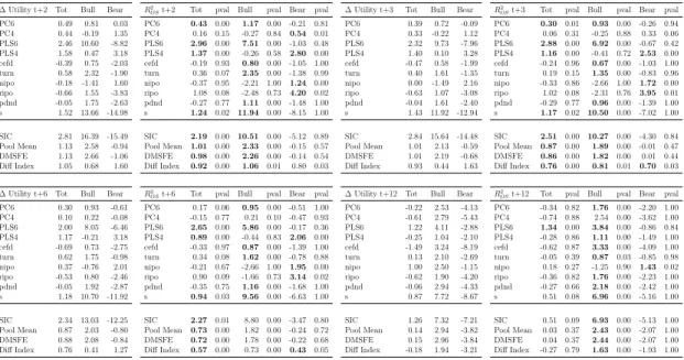
We start our empirical analysis in the simplest way: we take monthly returns and volumes data for the S&P500 for the period 01-1982/12-2015, we detrend volumes to account for the structural increase in volumes through the period considered and we divide our data into four sets, one for each possible combination between the dynamics of prices and volumes (positive/negative returns and rising/declining volumes). After that for each of the four monthly categories in which we have di-vided our sample, we compute the average return recorded by the S&P500 one month, three months and six months after the starting month. To provide an even more comprehensive picture, we also provide the cumulated returns spanning from month t+1 to month t+3, from month t+1 to month t+6 and from month t+4 to month t+6.

Insert T able2.1

Table 2.1 provides a first representation of the impact of the dichotomy on the

US financial markets. It is immediate to see the different impact of the rising volumes in bullish and bearish markets in predicting subsequent market returns. We observe how rising volumes, joined with negative returns, are evidence of a strong bearish movement which is likely to continue while rising volumes, joined with positive returns, are followed on average by subsequent high returns. Con-sequently, the impact of a high level of uncertainty on subsequent market returns depends on the prevailing market regime. Declining volumes matched by negative returns are evidence of a bearish market which is likely to revert and we report how they over perform, in terms of average returns, increasing volumes matched by negative returns for all the subsequent considered horizons. When bullish markets are considered, we observe how at month t+1 the average return of the S&P500

33_Han_[₂₀₀₈_{] shows how options prices timely reflect investor sentiment}

34_{This idea is first introduced in the seminal work of}_{Diether et al.}_[₂₀₀₂_{] and further developed}

(25)

following a month t characterized by rising volumes and positive returns is close to the performance following a month t characterized by declining volumes and positive returns. Crucially, when average returns at month t+3 are considered average returns are higher after a month t associated with positive returns and declining volumes than after a month t associated with positive returns and rising volumes, while the reverse applies for average returns at month t+6.

Our results imply that the dynamics of volumes and prices need to be scrutinized jointly because the existence of the dichotomy implies that uncertainty has a differ-ent informative contdiffer-ent in bullish and bearish markets. Months characterized by

negative returns and growing volumes are “fire sales” months (Shleifer and Vishny

[2011]) and, because of liquidity spirals, (Brunnermeier and Pedersen [2009]) and

cash flow based momentum (Vayanos and Woolley[2013]) are likely to be followed

by months characterized by poor returns. On the other hand, months with neg-ative returns and declining volumes imply that the bearish movement is ending or that is not robust enough to trigger liquidity spirals or massive fire sales: this implies that positive returns are likely to follow.

Even more interesting is the pattern which emerges when returns at time t are positive. At medium-short time horizons (months t+3), the average return of the following months (time t) characterized by declining volumes and positive returns over perform the average return following months characterized by rising volumes and positive returns, but the pattern reverse at longer horizons (t+6). This

ev-idence seems to point to a “calm before the storm” explanation (Akbas [2016]).

Indeed, when many investors enter the market in the same period (bullish market, rising volumes), a relevant share of investors expect markets to continue to rise.

Even more importantly loss aversion35explains why it is unlikely for these investors

to close their position in the following months if a negative shock arises. This re-duces the possibility of a major drawdown. On the other hand, after months of rising prices and declining volumes, it is more common for investors who entered before the low volumes months to cash in the gains as soon as negative returns materialize. Indeed, the most optimist investors are usually fully invested in the market: if these investors are mutual funds, they cannot employ leverage, while if they can employ leverage, they are already marking full use of it. Consequently, when the market declines leveraged investors cannot buy much more. Another possible interpretation is that unusually low trading volumes during bull markets signals negative information since, under short-selling constraints, informed agents

with bad news stay by the sidelines36_.

These results are coherent with the existing literature. Gervais et al.[2001] show

35_{The Prospect theory (}_{Kahneman and Tversky} _[₁₉₇₉_{]) and the related disposition effect}

(Shefrin and Statman[1985]) provide a solid rationale to these findings

(26)

how stocks which experience unusually high trading volumes over a day or a week tend to appreciate over the course of the following month. The specular applies for stocks which experience unusually low trading volumes. Differently from them, we consider aggregate market volumes and he discriminate between rising or declining de-trended volumes not very high (low) ones. Consequently, what we analyze is a different aspect of the issue while agreeing on the main point: because a lot of investors cannot go short when they are bearish, they simply do not invest in the

market reducing the volumes. Finally, Kaniel et al. [2008] prove that

individu-als tend to buy stocks following declines in the previous month and sell following price increases. The latter result is coherent with our understanding that, when a lot of investors has just bought stocks they are reluctant to sell and to realize losses in case negative returns occurs. Furthermore the authors also show how, in agreement with our findings, stocks register positive excess returns in the month following strong buying by individuals and negative excess returns after individuals strong sell.

2.4 Greed and Fear

In this section we study the empirical performance of the sentiment and fear proxies to understand what these indexes capture. At first, we examine their predictive

power both in and out-of-sample. Then, we analyze which are the drivers of

sentiment and fear and how they relate to uncertainty.

The first objects of study are sentiment proxies. To address what these indexes reflect we study how they interact with uncertainty. We aim at verifying whether rising sentiment relates to an increasing dispersion in the views (uncertainty). To study this relation, we make use of correlation, Granger causality, and lasso analysis among uncertainty proxies and sentiment indexes. After that, we analyze the existence of an uncertainty risk premium, and we consider the predictive power of uncertainty. Before proceeding with the formal analysis, we plot the time series of interest to gain first qualitative insights into the variables under study.

In Figure 2.1, upper part, we introduce the proxies considered in this study for

sentiment while in the same Figure, lower part, we provide a first visualization of the relationship between sentiment and uncertainty.

Insert F igure2.1

From Figure 1 emerges how all the sentiment proxies exhibit a procyclical dy-namic: they pick at the end of prolonged bull markets, and bottom after market crashes. Interestingly, after the financial crisis of 2008, the PC 6 sentiment proxy remains well below its long-term average despite an extremely prolonged period of rising markets. In the same period, all other sentiment proxies stayed in a more

(27)

conservative range and close to their historical average. The lower part of Figure

2.1 shows us how sentiment and uncertainty proxies are closely related: they

ex-hibit similar patterns both during bull and bear markets. Consequently, Figure

2.1 seems to suggest that the dispersion of investors views is linked to sentiment.

We also report a surprising fact: sentiment indicators proposed by the existing lit-erature (PC 6 and PLS 6) appear to spike right in the middle of some of the most violent market downturns of the last decades. These findings lead us to consider carefully the role played by the constituents from which the sentiment indexes are estimated. A deep investigation tells us that two (turnover and number of IPOs) of the six proxies initially employed are biased proxies of sentiment. First, share turnover is very high both in bull and in bear markets and, accordingly to our anal-ysis of the previous section, the dynamics of volumes should be analysed jointly with the market dynamics to be insightful about future expected returns. Second, the ’number of IPOs’ is largely driven by historical dynamics, like the dot.com wave or the development of a specific country or sector. Consequently, we argue that the number of IPOs is a biased proxy for sentiment. In the online appendix (

Figure 2.3), we provide a visualization of our intuition: we plot the time series of

turnover and of the number of IPOs with the sentiment proxy estimated using the Principal Component methodology and the remaining four sentiment indicators initially proposed by Baker and Wurgler. We observe how after the IPOs wave of the late nineties, the last few years of the sample which are characterized by extraordinarily high returns are matched by a relatively low number of IPOs in the US. In conclusion, we propose to estimate the sentiment indexes making use of only four of the six sentiment proxies originally proposed by Baker and Wurgler:

these new indexes (PC4 and PLS4) are both plotted in Figure 2.1 next to the

original ones (PC6 and PLS6).

The second object of study regards the fear proxies. As previously stated, the dichotomy between representative and marginal investor implies that it is not pos-sible to accurately extrapolate fear from the stock market: the most optimistic investors can in fact express themselves directly on stock markets buying stocks, but the same does not apply to the most pessimistic ones. On the other hand, the opaqueness of over the counter markets foreshadows the possibility to extrapolate reliable information from that side. To circumvent these limitations, we rely on surveys which explicitly address the concerns of the investors and on the options market which is both transparent and liquid. The nature of the options market and the composition of the pool of investors who work on it make the option market perfectly suitable for those analyses that are not feasible on the stock exchange. The existence of liquid put and call options with different maturities and moneynesses, allows traders to express their views without the constraints at the base of the dichotomy between marginal and representative investors. As a

(28)

consequence the left tail of the risk-neutral distribution emerges as a natural can-didate for better understanding the nature of fear and its relation with downward

uncertainty about fundamentals. Johnson et al. [2018] analyze the demand for

options in the market and conclude that the primary function of index options is

the transfer of unspanned crash risk. A vast literature37 _{finds that while the left}

tail of the distribution has a strong predictive content the same is not true for the right tail of the risk-neutral distribution. The asymmetry occurs because the optimist investors can freely express themselves on the stock market and they do not need to make use of options to speculate on optimistic views. After that, the percentage of investors which is short on the market is a low fraction of the total, and consequently, the need to hedge against markets upside movements is limited. As done previously for sentiment, we start our analysis of fear indexes from visual

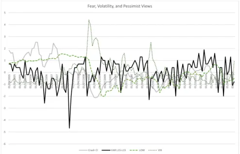
inspection. Figure 2.2, upper part, shows how fear proxies interact with volatility

and with the lower bound of the analysts’views. The lower part of the same Figure, shows how fear proxies relate to uncertainty measures.

Insert F igure2.2

Figure2.2shows how, while linked, volatility and fear are two separate phenomena.

It also show how the lower bound of the EPS long term growth views (LOW in the Figure) follows a path close to the fear measures ones. Furthermore, the lower plot reports how the downward uncertainty proxy is closely linked to the FVaR proxy while the financial uncertainty proxy (UF, in the Figure) is closely matched by the Crash Confidence Index measure of fear.

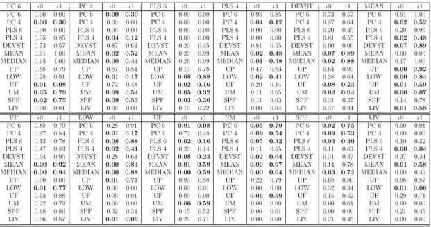
To better define the relation among measures of sentiment, fear, and uncertainty we analyze the correlation between sentiment and uncertainty variables and between

fear and uncertainty ones (Table 2.2).

Insert T able2.2

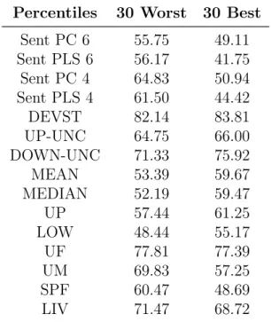
From the upper panel of Table 2.2 emerges how all sentiment indexes exhibit a

strong positive correlation among themselves. Secondly, it is immediately clear how the weighted standard deviation of the forecast (DEVST) is more positively correlated with the upper bound of the forecasts than negatively correlated with the lower bound of the forecasts. Consequently, the upper bound of the views appears to affect the dispersion of the views more than the lower bound. Af-ter that, we observe how correlations between sentiment indexes and uncertainty proxies are positive (UF, UM, SPF, LIV) or close to zero (DEVST, UP-UNC, DOWN-UNC). Finally, the uncertainty proxies, as expected, are positively corre-lated among themselves.

37_{See, e.g.,} _{Andersen et al.}_[₂₀₁₅_], _{Bollerslev et al.}_[₂₀₁₅_] _{Christoffersen et al.}_[₂₀₁₂_], _Amaya

(29)

Three main findings emerge from the lower panel of Table2.2. First, option-based measures of fear are positively correlated among themselves (VaR L15-L15, BTX, FFHS, VRP, VIX). Second, the correlations between our newly proposed fear proxies (FFHS, VaR L15-L15, TAIL) and the lower bound of analysts forecast are higher than the correlations between the same fear proxies and the upper bound of analysts forecasts. The asymmetry is clear evidence that the most optimist and the most pessimist investors react differently to changes in the aggregate market risk aversion, a result coherent with what we found in our previous analysis of

sentiment where our results are specular (upper panel of Table 2.2). Third, the

correlations between fear proxies (Bull-Bear, CRASH, FVaR, FFHS) and uncer-tainty ones (UM, UF, DEVST) are negative or close to zero, and the results are

stronger conditionally on a decline of the FVaR measure38_.

To unveil what our sentiment, fear and uncertainty proxies capture we start

study-ing their predictive performance out of sample usstudy-ing the R2

os and delta utility

met-rics. The former metric is further decomposed to disentangle the capability of the

proxy to forecast positive and negative returns only (Bull and Bear in Table 2.3).

For the analysis, the out-of-sample performance metrics considered are:

• The R2

os statistic proposed by Campbell and Thompson [2008]

R2_os= 1 − PT t=1(rt− ˆrt) 2 PT t=1(rt− ¯rt)2 (2.11) R2

os measures the percent reduction in mean squared forecast error (MSFE)

between the forecasts generated by the chosen predictive model, ˆr, and the

historical average benchmark forecast, ¯r. To assess the statistical

signifi-cance of R2

os we employ the p-values coming from the Clark and West (2007)

MSFE-adjusted statistic. This indicator tests the null hypothesis that the historical average MSFE is less than or equal to the forecasting method MSFE against the alternative that the historical average MSFE is greater

than the forecasting method MSFE (corresponding to H0 : R2os 6 0 against

H1 : Ros2 > 0).

• The Delta Utility measure proposed by Campbell and Thompson (2008)

Camp-bell and Thompson [2008]. Following the original paper, we estimate the

variance using a ten-year rolling window of returns. We consider a mean-variance investor who forecasts the equity premium using the historical av-erages. She will decide at the end of period t to allocate the following share

38_{The tables which report conditional correlation are reported in the online appendix (Table}

(30)

of her portfolio to equity in the subsequent period t+1: w0,t = 1 γ ¯ rt+1 ˆ σt+1 (2.12)

where ˆσt+1 is the rolling-window estimate of the variance of stock returns.

Over the out-of-sample period, she will obtain an average utility of: ˆ v0 = ˆµ0− 1 2γ ˆσ 2 0 (2.13)

where ˆµ0 and ˆσ02 are the sample mean and variance, over the out-of-sample

period for the return on the benchmark portfolio formed using forecasts of the equity premium based on the historical average. Then we compute the average utility for the same investor when she forecasts the equity premium using one of the predictive approaches proposed in this paper. In this case, the investor will choose an equity share of:

wj,t = 1 γ ˆ rt+1 ˆ σt+1 (2.14) and she will realize an average utility level of:

ˆ vj = ˆµj− 1 2γ ˆσ 2 j (2.15)

where ˆµ and ˆσt+1 are the sample mean and variance, over the out-of-sample

period for the return on the portfolio formed using forecasts of the equity premium based on one of the methodologies proposed. In this paper, we

measure the utility gain as the difference between ˆvj and ˆv0, and we multiply

this difference by 100 to express it in average annualized percentage return.

In our analysis, following the existing literature39_{, we report results for γ = 3.}

To make our results comparable, in light of the heterogeneity of the length of the different time series considered, we apply the same percentages to split each time series into an in sample, hold out and out-of-sample period: 40%, 10% and 50% respectively.

Insert T able2.3

The results of the out-of-sample predictive performance are extremely insightful.

Table2.3shows how, overall, the most powerful predictor among sentiment proxies

39_{Among the most cited works on the subject} _{Campbell and Thompson} _[₂₀₀₈_{] and} _Rapach

(31)

employs six inputs and the PLS approach (R2_OS=2.11). Interestingly, disaggregat-ing the overall predictive ability (Tot) in the capability to forecast positive (Bull) or negative (Bear) returns only, other results emerge. At first, it appears how

original sentiment proxy of Baker and Wurgler [2006] (PC6) is more effective in

forecasting positive (R2

OS=0.80) than negative returns (R2OS=-0.03). Similarly, the

turnover variable is powerful in predicting positive returns (R2

OS=2.31) and weak

in predicting negative ones (R2_OS=-1.30). The omission of this variable40 makes

the PC 4 and PLS 4 sentiment proxies good predictors for bear markets and weak predictors for bull ones. Consequently, the capability to forecast correctly bear markets but not bull ones means that the PC 4 and PLS 4 indexes capture overbought situations or situations of abnormally low risk aversion. The PLS 6

sentiment proxy presents a similar performance (Bull R2

OS=0.42, Bear R2OS=3.47)

and this implies that the employment of a more powerful statistical procedure (PLS) is a viable alternative in effectively synthesizing the predictive power of the six original proxies for sentiment into an effective overbought indicator.

Then we analyze the predictive power of uncertainty proxies. The obtained re-sults are aligned and clear: while overall their predictive performance is weak, all the financial and macroeconomic uncertainty indexes are effective in forecasting negative returns but not positive ones. The evidence that the overall predictive performance is weak is in line with our previous finding that high uncertainty precedes both positive and negative returns depending on the prevailing market conditions. Moreover, the capability to forecast negative but not positive returns is in line with the predictive ability of the PC 4, PLS 4 and PLS 6 proxies for sen-timent and confirms the strong links between sensen-timent and uncertainty proxies. We now study fear proxies. Here the most powerful predictors are option-based:

FVaR (R2

OS=9.54), FCVaR (R2OS=18.79), and VRP (R2OS=6.06). When we

dis-entangle the overall predictive performance in the capability to forecast positive and negative returns, we observe how a clear pattern emerges. The indexes which make use of surveys (UM-MD, the LIV Skew, the RGDPX Skew, CRASH) and the indexes that make use of option implied information (FFHS, FVaR, FCVaR) achieve a robust predictive performance in forecasting positive returns and a weak performance in predicting negative ones. On the other hand, stock based indexes (TAIL, KJ, CATFIN), the MACRO uncertainty proxy, and the Anxious index (ANX) are all better able to forecast negative than positive returns. Finally, the VIX index shows no sign of having a predictive power, while the variance risk pre-mium (VRP) has an overall positive and statistically significant predictive power coming from its ability to forecast both negative and positive returns. Overall, the predictive performances out-of-sample of the indexes considered lead us to classify them in two categories: indexes of uncertainty, which concentrate their predictive