Simulations of preindustrial, present-day, and 2100 conditions in the NASA GISS composition and climate model G-PUCCINI

(1)

HAL Id: hal-00297184

https://hal.archives-ouvertes.fr/hal-00297184

Submitted on 4 Oct 2006

HAL is a multi-disciplinary open access

archive for the deposit and dissemination of

sci-entific research documents, whether they are

pub-lished or not. The documents may come from

teaching and research institutions in France or

abroad, or from public or private research centers.

L’archive ouverte pluridisciplinaire HAL, est

destinée au dépôt et à la diffusion de documents

scientifiques de niveau recherche, publiés ou non,

émanant des établissements d’enseignement et de

recherche français ou étrangers, des laboratoires

publics ou privés.

conditions in the NASA GISS composition and climate

model G-PUCCINI

D.T. Shindell, G. Faluvegi, N. Unger, E. Aguilar, G.A. Schmidt, D.M. Koch,

S.E. Bauer, R.L. Miller

To cite this version:

D.T. Shindell, G. Faluvegi, N. Unger, E. Aguilar, G.A. Schmidt, et al.. Simulations of preindustrial,

present-day, and 2100 conditions in the NASA GISS composition and climate model G-PUCCINI.

Atmospheric Chemistry and Physics, European Geosciences Union, 2006, 6 (12), pp.4427-4459.

�hal-00297184�

(2)

www.atmos-chem-phys.net/6/4427/2006/ © Author(s) 2006. This work is licensed under a Creative Commons License.

Chemistry

and Physics

Simulations of preindustrial, present-day, and 2100 conditions in the

NASA GISS composition and climate model G-PUCCINI

D. T. Shindell1,2, G. Faluvegi1,2, N. Unger1,2, E. Aguilar1,2, G. A. Schmidt1,2, D. M. Koch1,3, S. E. Bauer1,2, and R. L. Miller1,4

1_{NASA Goddard Institute for Space Studies, New York, NY, USA}

2_{Center for Climate Systems Research, Columbia University, NY, USA}

3_{Dept. of Geophysics, Yale University, New Haven, USA}

4_{Dept. of Applied Physics and Applied Math, Columbia University, NY, USA}

Received: 3 February 2006 – Published in Atmos. Chem. Phys. Discuss.: 15 June 2006 Revised: 14 September 2006 – Accepted: 26 September 2006 – Published: 4 October 2006

Abstract. A model of atmospheric composition and climate has been developed at the NASA Goddard Institute for Space Studies (GISS) that includes composition seamlessly from the surface to the lower mesosphere. The model is able to capture many features of the observed magnitude, distribu-tion, and seasonal cycle of trace species. The simulation is especially realistic in the troposphere. In the stratosphere, high latitude regions show substantial biases during period when transport governs the distribution as meridional mix-ing is too rapid in this model version. In other regions, in-cluding the extrapolar tropopause region that dominates ra-diative forcing (RF) by ozone, stratospheric gases are gen-erally well-simulated. The model’s stratosphere-troposphere exchange (STE) agrees well with values inferred from obser-vations for both the global mean flux and the ratio of North-ern (NH) to SouthNorth-ern Hemisphere (SH) downward fluxes.

Simulations of preindustrial (PI) to present-day (PD) changes show tropospheric ozone burden increases of 11% while the stratospheric burden decreases by 18%. The result-ing tropopause RF values are −0.06 W/m2from stratospheric

ozone and 0.40 W/m2from tropospheric ozone. Global mean

mass-weighted OH decreases by 16% from the PI to the PD. STE of ozone also decreased substantially during this time, by 14%. Comparison of the PD with a simulation using 1979 pre-ozone hole conditions for the stratosphere shows a much larger downward flux of ozone into the troposphere in 1979, resulting in a substantially greater tropospheric ozone burden than that seen in the PD run. This implies that reduced STE due to stratospheric ozone depletion may have offset as much as 2/3 of the tropospheric ozone burden increase from PI to PD. However, the model overestimates the downward flux of

Correspondence to: D. T. Shindell

(dshindell@giss.nasa.gov)

ozone at high Southern latitudes, so this estimate is likely an upper limit.

In the future, the tropospheric ozone burden increases by 101% in 2100 for the A2 scenario including both emissions and climate changes. The primary reason is enhanced STE, which increases by 124% (168% in the SH extratropics, and 114% in the NH extratropics). Climate plays a minimal role in the SH increases, but contributes 38% in the NH. Chem-istry and dry deposition both change so as to reduce tropo-spheric ozone, partially in compensation for the enhanced STE, but the increased ozone influx dominates the burden

changes. The net RF due to projected ozone changes is

0.8 W/m2for A2. The influence of climate change alone is

−0.2 W/m2, making it a substantial contributor to the net RF.

The tropospheric oxidation capacity increases seven percent in the full A2 simulation, and 36% due to A2 climate change alone.

1 Introduction

There are many ways in which changes in atmospheric com-position and climate are coupled. The interactions are es-pecially pronounced in the case of chemically reactive gases and aerosols. For example, atmospheric humidity increases as climate warms, altering reactions involving water vapor and aqueous phase chemistry in general, which in turn af-fects the abundance of radiative active species such as ozone and sulfate. Additional couplings exist via climate-sensitive natural emissions, such as methane from wetlands and iso-prene from forests, aerosol-chemistry-cloud interactions in a changing climate, and large-scale circulation shifts in re-sponse to climate change, such as stratosphere-troposphere

(3)

exchange (STE). This paper presents the latest version of the NASA Goddard Institute for Space Studies (GISS) compo-sition and climate model as part of our continuing efforts to more realistically simulate the range of physical interactions important to past, present and future climates.

The trace gas photochemistry has been expanded from the earlier troposphere-only scheme described in Shindell et al. (2001, 2003) to include gases and reactions impor-tant in the stratosphere. This builds upon previous model-ing of tropospheric or stratospheric chemistry within GCMs (e.g. Austin et al., 2003; Stevenson et al., 2006) and initial work including both tropospheric and stratospheric chem-istry (e.g. Dameris et al., 2005). At the same time, the sulfate aerosol and trace gas chemistry have been fully coupled (Bell et al., 2005) and interactions between chemistry and mineral dust have been added to the model. Climate-sensitive

emis-sions have been included for methane from wetlands, NOx

from lightning, dust from soils, and DMS from the ocean. Water isotopes and a passive linearly increasing tracer have

been included, allowing better transport diagnostics. All

components have been developed within the new GISS mod-elE climate model (Schmidt et al., 2006). Since the climate model developed under the modelE project has been named GISS model III, and the chemistry is also the third major version of its development following Shindell et al. (2001, 2003), it is appropriate to call this model the GISS composi-tion and climate model III. We prefer, however, a more de-scriptive name: the GISS model for Physical Understand-ing of Composition-Climate INteractions and Impacts (G-PUCCINI).

We present a detailed description of the model in Sect. 2, followed by an evaluation against available observations in Sect. 3. Section 4 presents the response to preindustrial and 2100 composition and climate changes as an initial applica-tion of this model. We conclude with a discussion of the model’s successes and limitations with an eye towards deter-mination of the suitability of the current model for various potential future studies.

2 Model description

2.1 Trace gas and aerosol chemistry

The trace gas photochemistry has been expanded from the tropospheric scheme developed previously (Shindell et al., 2001a, 2003) to include species and reactions important in

the stratosphere. Table 1 lists the molecules included in

the gas photochemistry. Table 2 presents the additional 78 new reactions incorporated within the chemistry scheme. Together with the reactions included previously, the pho-tochemistry now includes 155 reactions. Rate coefficients are taken from the NASA JPL 2000 handbook (Sander et al., 2000). Photolysis rates are calculated using the Fast-J2 scheme (Bian and Prather, 2002), except for the photolysis of

water and nitric oxide (NO) in the Schumann-Runge bands, which are parameterized according to Nicolet (1984) and Nicolet and Cieslik (1980). The chemical solver is a hybrid of equilibrium calculations for the shortest-lived radicals, an interative calculation for a few species with intermediate life-times, and an explicit calculation for longer-lived species. Transported species are advected using second-order mo-ments (Prather, 1986), which is able to maintain large gra-dients and in essence provides information at a substantially higher (∼4×) resolution than the GCM grid.

Heterogeneous chemistry in the stratosphere follows the reactions listed in Table 2. Aerosol surface areas are set to match those used in the GCM’s calculation of radiative transfer based upon an updated version of the volcanic plus background aerosol timeseries of Sato et al. (1993). Sur-face areas for polar stratospheric clouds (PSCs) are set us-ing simple temperature thresholds for type I and II particles, 195 and 188 K, respectively, with a parameterization of sed-imentation also included. A more sophisticated model based on Hanson and Mauersberger (1988) is being incorporated into the chemistry code, but is not yet functional. Thus the simulations do not include all potential pathways for interac-tions between polar ozone chemistry and climate or emis-sions changes as PSC formation is not sensitive to water or nitric acid abundance variations. Given that the model’s transport biases limit the realism of its polar ozone simula-tions in any case, it was deemed a better use of resources to address this in future higher resolution runs than to repeat these simulations with a more advanced PSC scheme.

Chemistry can be included in the full model domain, or it can be restricted to levels below the meteorological tropopause. In the latter case, climatological ozone is used in the stratosphere and NOxis prescribed as a fixed fraction

of the ozone abundance as in our previous models. While we focus on the full chemistry model, both configurations are evaluated here so that future studies can select the most appropriate version.

To better understand the model’s simulation of strato-spheric transport, we have incorporated a passive, linearly increasing tracer as a standard feature along with the chemi-cal tracers. This tracer is initialized in the lowest model layer with a value that increases by one unit each year, with a lin-ear interpolation used to set monthly values. The difference between the tracer value at a given point and the surface level value then gives the mean time in years since the air left the surface. By comparing values throughout the stratosphere with those at the tropical tropopause, we can evaluate the age of air in the stratosphere and compare with observations of CO2and SF6.

The updated modelE version of the sulfate and sea salt model is described and evaluated by Koch et al. (2006), though in those simulations the aerosols were not cou-pled with chemistry. It includes prognostic simulations of

DMS (dimethyl sulfide), MSA (methane sulfonic acid), SO2

(4)

Table 1. Gases included in the model.

Transported Not Transported

(1) Ox (28) NO (2) NOx (29) NO2 (3) HNO3 (30) NO3 (4) N2O5 (31) HONO (5) HO2NO2 (32) OH (6) H2O2 (33) HO2 (7) CO (34) O (8) HCHO (35) O(1D) (9) CH3OOH (36) O3 (10) H₂O (37) CH₃O₂ (11) CH4 (38) C2O3 (12) PANs (39) Aldehydesa (13) Isoprene (40) XOd₂ (14) Alkyl Nitratesa (41) XO2Ne (15) Alkenesa (42) RXPARf (16) Paraffinsa (43) RORg (17) ClOx (44) Cl (18) BrOx (45) ClO (19) HCl (46) OClO (20) HOCl (47) Cl2O2 (21) ClONO2 (48) Cl2 (22) HBr (49) ClNO₂ (23) HOBr (50) Br (24) BrONO₂ (51) BrO (25) N2O (52) BrCl (26) CFCsb (53) N

(27) Linearly increasing tracerc (54) H

a_{Alkyl nitrates, alkenes, paraffins, and aldehydes are lumped families. Alkenes include propene, >C3 alkenes, and >C2 alkynes,} paraf-fins include ethane, propane, butane, pentane, >C5 alkanes and ketones, while aldehydes include acetaldehyde and higher aldehydes (not formaldehyde).

b_{CFCs are defined here as the sum of all CFCs, using the characteristics of CFC-11.}

c_{Linear tracer is a tracer with a linearly increasing surface abundance that can be scaled to SF}

6or CO2to evaluate the models age of air against observations.

d_XO

2is a surrogate species to represent primarily hydrocarbon oxidation byproducts that subsequently convert NO to NO2, and also leads to a small amount of organic peroxide formation.

e_XO

2N is a surrogate species to represent hydrocarbon oxidation byproducts that subsequently convert NO to alkyl nitrates, and also leads to a small amount of organic peroxide formation.

f_{RXPAR is a paraffin budget corrector to correct a bias in the oxidation of alkenes related to an overly short chain length for the lumped} alkenes.

g_{ROR are radical byproducts of paraffin oxidation.}

chemistry and aerosols in this model has been investigated extensively (Bell et al., 2005). The mineral dust aerosol model transports four different sizes classes of dust particles with radii between 0.1–1, 1–2, 2–4, and 4–8 microns. Par-ticle sources are identified using the topographic prescrip-tion of (Ginoux, 2001). Direct dust emission increases with the third power of the wind speed above a threshold that in-creases with soil moisture. Emission is calculated by inte-grating over a probability distribution of surface wind speed that depends upon the speed explicitly calculated by the GCM at each grid box, along with the magnitude of

fluctua-tions resulting from subgrid circulafluctua-tions created by boundary layer turbulence, and dry and moist convection. Dust parti-cles are removed from the atmosphere by a combination of gravitational settling, turbulent mixing, and wet scavenging. Dust also affects the radiation field, and thus influences pho-tolysis rates. A more detailed description of the dust model, along with a comparison to regional observations, is given by Miller et al. (2006) and Cakmur et al. (2006).

The model includes heterogeneous chemistry for the up-take of nitric acid on mineral dust aerosol surfaces. This is described by a pseudo first-order rate coefficient which gives

(5)

Table 2. Additional reactions included in the model.

Bimolecular Reactions (1) Cl + O3→ClO + O2 (2) ClO + O → Cl + O2 (3) Cl + OClO → ClO + ClO (4) ClO + O3→ClOO + O2 (5) ClO + O₃→OClO + O₂ (6) O + OClO → ClO + O2 (7) OH + Cl2→HOCl + Cl (8) OH + HCl → H2O + Cl (9) OH + HOCl → H2O + ClO (10) O + HCl → OH + Cl (11) O + HOCl → OH + ClO (12) OClO + OH → HOCl + O₂ (13) Cl + HOCl → Cl2+ OH (14) Cl + H2O2→HCl + HO2 (15) Cl + HO2→HCl + O2 (16) Cl + HO2→OH + ClO (17) ClO + OH → HO2+ Cl (18) ClO + OH → HCl + O2 (19) ClO + HO₂→HOCl + O₂ (20) ClO + NO → NO2+ Cl (21) ClONO₂+ O → ClO + NO₃ (22) HCl + O(1D) → Cl + OH (23) NO + OClO → NO₂+ ClO (24) HBr + OH → H2O + Br (25) BrO + O → Br + O2 (26) Br + O3→BrO + O2 (27) BrO + NO→Br + NO2 (28) Br + HO2→HBr + O2 (29) BrO + HO2→HOBr + O2 (30) Br + OClO → BrO + ClO (31) BrO + ClO → OClO + Br (32) BrO + ClO → Br + ClOO (33) BrO + ClO → BrCl + O2 (34) BrO + BrO → Br + Br (35) Br + H2O2→HBr + HO2 (36) BrO + OH → Br + HO2 (37) BrO + OH → HBr + O₂ (38) Cl + CH4→HCl + CH3O2 (39) Cl + H₂→HCl + H (40) O + HBr → OH + Br

(41) ClO + CH3O2→ClOO + HCHO + HO2 (42) N2O + O(1D) → N2+ O2 (43) N2O + O(1D) → NO + NO (44) O + O3→O2+ O2 (45) O + OH → O2+ H (46) O + HO₂→OH + O₂ (47) N + O2→NO + O (48) N + NO₂→N₂O + O (49) N + NO → N2+ O (50) H + O3→OH + O2 (51) H + O2+ M → HO2+ M (52) ClO + ClO → Cl2+ O2 (53) ClO + ClO → ClOO + Cl (54) ClO + ClO → OClO + Cl (55) O + H₂O₂→ Monomolecular reactions (56) Cl₂O₂+ M → ClO + ClO + M Termolecular reactions (57) ClO + ClO + M → Cl2O2+ M (58) ClO + NO2+ M → ClONO2+ M (59) BrO + NO₂+ M → BrONO₂+ M Heterogeneous reactions (60) N₂O₅+ H₂O → HNO₃+ HNO₃ (61) ClONO2+ H2O → HOCl + HNO3 (62) ClONO₂+ HCl → Cl₂+ HNO₃ (63) HOCl + HCl → Cl2+ H2O (64) N2O5+ HCl → ClNO2+ HNO3 Photolysis Reactions (65) ClO + hν → Cl + O (66) Cl2+ hν → Cl + Cl (67) OClO + hν → O + ClO (68) Cl2O2+ hν → Cl + Cl + O2 (69) HOCl + hν → OH + Cl (70) ClONO2+ hν → Cl + NO3 (71) BrONO2+ hν → BrO + NO2 (72) HOBr + hν → Br + OH (73) BrO + hν → Br + O (74) CFC + hν → Cl (75) O2+ hν → O + O (76) N2O + hν → N2+ O(1D) (77) NO + hν → N + O (78) H2O + hν → OH + H M is any body that can serve to carry away excess energy. ClOO is assumed to decay immediately to Cl + O2.

the net irreversible removal rate of gas-phase species to an aerosol surface. We use the uptake coefficient of 0.1 recom-mended from laboratory measurements (Hanisch and Crow-ley, 2001), though this value is fairly uncertain. The effects of mineral dust on sulfate have been described elsewhere (Bauer and Koch, 2005). The model includes simulations of carbonaceous, sea-salt and nitrate aerosols as well, though

these do not directly influence the simulations of other trace species in the model and are described in detail elsewhere (Koch and Hansen, 2005; Koch et al., 2006).

The model also includes the stable water isotopes HDO

and H18₂ O, which are fully coupled to the GCM’s

hydro-logic cycle. Comparison between the modeled and observed values of these isotopes, and especially of their vertical

(6)

Table 3. Simulations with the full chemistry model.

Long-lived gases Short-lived

Year CO2 N2O CH4 CFC species Ocean ppmv ppbv ppmv ppbv emissions conditions

Evaluation runs

Present-day (PD) 1995 360.7 315.7 calc 3.2 1990s 1990s 1979 stratosphere 1979 337.1 300.9 1.53 1.2* 1990s responsive

Climate runs

Preindustrial (PI) 1850 285.2 275.4 0.79 0.0 ∼1850 responsive Present-day (PD) 1995 360.7 315.7 ∼1.85 N 3.2 1990s responsive

∼1.72 S

A2 emissions and climate 2100 856.0 447.0 3.731 1.2 2100 responsive A2 climate-only NA 856.0 315.7 ∼1.85 N 3.2 1990s 2100

∼1.72 S

* This value represents approximately the CFC loading that had reached the stratosphere in 1979. Calc=calculated.

profiles, can be a useful way to evaluate (and improve) the stratosphere-troposphere exchange in the model and the parameterization of cloud physics (Schmidt et al., 2005).

An important new feature of modelE for the trace gas and aerosol species is a carefully constructed cloud tracer bud-get. Most chemical and aerosol models (including all GISS models other than modelE) do not save dissolved species in a cloud budget but instead return the dissolved (unscavenged) species to the model grid box at the end of each model time-step. In our model, we have created a cloud liquid budget and this has important implications for tracer distributions. Inclusion of the cloud tracer budget decreases sulfate pro-duction in the clouds (since most of the sulfate is ultimately rained out instead of released back to the grid box) (Koch et al., 2006) and reduces the abundance of soluble O3

precur-sors, such as nitric acid (HNO3), which were systematically

overestimated in previous models. We have also developed a new dry deposition module within modelE that is physically consistent with the other surface fluxes (e.g. water, heat) in the planetary boundary layer scheme of the GCM, which was not the case in earlier models (or indeed in most chemistry-climate models).

2.2 Sources and sinks

Emissions of trace gases and aerosols are largely the same as those used in previous versions (Shindell et al., 2003). They include the standard suite of emissions from fossil fuel and biomass burning, soils, industry, livestock, forests, wetlands, etc. These are based largely on GEIA inventories (Benkovitz et al., 1996). Sulfur emissions are from the EDGAR inven-tory as described in Bell et al. (2005). For the new long-lived species included here, N2O and CFCs (and CO2), we

pre-scribe values at observed amounts (Table 3) in the lowest model layer. This technique is also available for methane, though in the present-day simulations described here we use the full set of methane emissions. CFCs are modeled using

the characteristics of CFC-11 but with a magnitude designed to capture the total chlorine source from all CFC species (i.e. each CFC yields one chlorine atom when broken down, so the amount of CFCs is set to match total anthropogenic chlorine). We also assume there is a background chlorine value of 0.5 ppbv from natural sources throughout the strato-sphere. Total bromine is normalized to prescribed loading (World Meteorological Organization, 2003) throughout the stratosphere.

2.3 Climate model

During the past several years, primary GISS modeling ef-forts have been directed into an entirely rewritten and up-graded climate model under the modelE project (Schmidt et al., 2006). This resulting GISS model, called either mod-elE or model III, incorporates previously developed physical processes within a single standardized structure quite differ-ent from the older model. This structure is much more com-plicated to create, but makes the interaction between GISS model components easier and more physically realistic. The standardization across components has also allowed many improvements to be included relatively easily.

ModelE also includes several advances compared to previ-ous versions, including more realistic physics and improved convection and boundary layer schemes. The horizontal res-olution can be easily altered, unlike previous versions. Stan-dard diagnostics include statistical comparisons with satel-lite data products such as ISCCP cloud cover, cloud height, and radiation products, MSU temperatures, TRMM precip-itation, and ERBE radiation products. Over a full suite of evaluation comparisons, including the satellite data and stan-dard reference climatologies for parameters such as circu-lation, precipitation, snow cover, and water vapor, modelE now substantially outperforms all other GISS model ver-sions (of course not on every individual quantity), producing rms errors approximately 11% less than those for Model II0.

(7)

-90 -75 -60 -45 -30 -15 0 15 30 45 60 75 90 .5 1.0 1.5 2.0 2.5 3.0 3.5 4.0 4.5 5.0 5.5 6.0 min max gsfc3d uiuc uci23 gsfc2d harvd monash1 co2(ER2) sf6(ER2) giss

20 km

Latitude

mean age (years)

0. 1.0 2.0 3.0 4.0 5.0 6.0 7.0 8.0 20 25 30 min max gsfc3d uiuc uci23 gsfc2d harvd monash1 sf6(44N) sf6(35N) co2(35N) giss

40N

mean age (years)

z(km)

Fig. 1. Comparison of the modeled age of air with other models and data from Hall et al. (1999). The data (symbols) are based on CO2 and SF6observations as per the references in the text. The “min” and “max” lines show the range of mean ages of models other than those explicitly plotted here. The current model is in blue.

The new modelE GCM was used for the GISS simulations performed for the forthcoming Intergovernmental Panel on Climate Change (IPCC) Fourth Assessment Report (AR4). Hence this model has been scrutinized in great detail, so that the behavior of physical processes have been compared with a wide range of observations and the model’s response to a large number of forcings has been well-characterized.

Yet another important feature of modelE is the capability to run the GCM with linear relaxation, or “nudging”, to re-analysis data for winds. This allows the model’s meteorology to be forced to match fairly closely that which existed during particular times, making for a much cleaner comparison with observational datasets.

GISS model development has benefited particularly from the close interaction of the composition modelers with the basic climate model developers at all stages, which has en-abled development of many consistent physical linkages such as the surface fluxes and liquid tracer budgets.

2.4 Experimental setup for model evaluation

We use a model version with 23 vertical layers (model top in the mesosphere at 0.01 hPa) and 4×5 degree horizontal resolution. Present-day simulations use seasonally varying climatological sea surface temperatures and sea ice cover-age representative of the 1990s, and were run with constant boundary conditions (an equilibrium simulation) for 20 years following an 18 year spinup (Table 3). All of the simulations described here use the GCM’s internally generated meteoro-logical fields (i.e. none have been relaxed towards reanalysis fields).

For all the simulations described here, we use the strato-spheric aerosol distribution for 1984, a mid-range year in terms of volcanic loading. For the tropospheric chemistry-only version, the stratospheric ozone climatology is set to 1990s levels. Additionally, the tropospheric chemistry-only simulations were run including interactive aerosols, which are coupled to the chemistry (Bell et al., 2005). Heteroge-neous chemistry on dust was included in a separate sensitiv-ity study to isolate its influence. Aerosol indirect effects were not included in these runs. In the full chemistry simulations, we revert to using offline prescribed aerosol fields for com-putational efficiency as the chemistry-aerosol coupling has a substantial effect on the aerosol simulation, but only a minor effect on the trace gases, which are our primary concern here (Unger et al., 2006).

The model has the capability to have changes in compo-sition affect radiative transfer for radiatively active species including ozone, methane, water, aerosols and dust (but not

NO2). The full chemistry simulations were performed

in-cluding such interactions. However, since the simulations we report on here for model evaluation used prescribed present-day sea surface temperatures (SSTs) and sea ice conditions, changes in the radiatively active gases could not affect cli-mate substantially, though they could influence atmospheric temperatures. In the climate simulations described in Sect. 4, however, this interaction becomes important.

3 Evaluation of present-day simulation 3.1 Long-lived gases in the stratosphere

Several long-lived species have been included as transported gases. These include nitrous oxide (N2O), a source of NOx

radicals in the stratosphere, methane (CH4)and water vapor

(H2O), sources of stratospheric HOx, and

(8)

Jan Apr Jul Oct Jan 0 90 -90 -0.8 -0.6 -0.4 -0.2 0 0.2 0.4 0.6 0.8 -40 -30 -20 -10 0 10 20 30 40 Latitude

Residual vertical velocity (mm/s)

Latitude

-45 45

Residual vertical velocity (mm/s)

0.15

Fig. 2. Annual mean (top) and seasonal cycle (bottom) of residual vertical velocity at 68 hPa. For the annual mean, the solid line is from UKMO analyses averaged over 1992–2001, while the dashed line is from the GCM present-day control run. Contours are .05 mm/s for positive values, .25 mm/s for negative. Areas with upwelling velocity >0.15 mm/s are shaded.

tracer to diagnose transport was also included. This is pre-sented in Fig. 1, which shows the age of air in the strato-sphere calculated using the linearly increasing tracer in com-parison with values derived from SF6and CO2observations

(Andrews et al., 1999; Boering et al., 1996; Elkins et al., 1996; Harnisch et al., 1996) and values from other models (Hall et al., 1999). Clearly the model’s air in the high lati-tude lower stratosphere is too young, a feature seen in most GCMs and even in CTMs driven by assimilated meteorolog-ical data (Scheele et al., 2005; Schoeberl et al., 2003).

The annual mean residual vertical velocity in the model underestimates the maximum values seen in the UKMO anal-yses (Swinbank and O’Neill, 1994), and the region of up-welling extends too far poleward in the SH, and to a much lesser extent in the NH (Fig. 2). The model’s mean up-welling velocity is 35% slower than in the observations. However, the seasonal cycle shows the maximum upwelling occurring in the summer subtropics in both hemispheres, in accord with Rosenlof (1995) and Plumb and Eluszkiewicz (1999). This simulation of the seasonality of tropical up-welling is a marked improvement over that seen in the older

GISS model II, which failed to reproduce the austral summer maximum entirely (Butchart et al., 2006). The model also simulates a local minimum in upwelling near the equator, a feature seen in most GCMs but not in previous GISS mod-els (Butchart et al., 2006). The underestimate of upwelling velocities indicates that air reaches the high latitude lower stratosphere too easily via meridional transport across the semi-permeable barriers in the stratosphere rather than via a Brewer-Dobson circulation that is too rapid.

Consistent with these circulation biases, the model’s zonal

mean N2O and CH4 distributions are too broad compared

with satellite climatologies from the Halogen Occultation Experiment (HALOE) and the Cryogenic Limb Array Etalon Spectrometer (CLAES) (Randel et al., 1998) (Fig. 3). Also, the high mixing ratio values entering the stratosphere in the tropics do not penetrate to high enough altitudes before be-ing chemically transformed. The distribution of CFCs in the model exhibits a similar shape. The weak meridional gra-dients in the distributions of these long-lived gases implies that transport across the subtropical and polar barriers is too rapid. Additionally, there may not be enough downward

(9)

HALOE + CLAES CH4 -90 -60 -30 0 30 60 90 LATITUDE 100.0 10.0 1.0 0.1 GCM CH4 -90 -60 -30 0 30 60 90 LATITUDE 100.0 10.0 1.0 0.1 0.00 0.20 0.60 1.00 1.40 1.80 CLAES N2O -90 -60 -30 0 30 60 90 LATITUDE 100.0 10.0 1.0 0.1 PRESSURE [hPa] GCM N2O -90 -60 -30 0 30 60 90 LATITUDE 100.0 10.0 1.0 0.1 PRESSURE [hPa] 0.00 0.04 0.08 0.12 0.16 0.20 0.00 3.50 4.50 5.50 6.50 7.50 HALOE+MLS H2O -90 -60 -30 0 30 60 90 LATITUDE 100.0 10.0 1.0 0.1 GCM H2O -90 -60 -30 0 30 60 90 LATITUDE 100.0 10.0 1.0 0.1

Fig. 3. Zonal mean April N₂O, CH₄and H₂O from satellite observations and in the model. All values are in ppmv. N₂O data is from the CLAES instrument, methane data from HALOE+CLAES, and water data from HALOE+MLS instruments. Tick marks along the right of the modeled water vapor distribution (lower right) show the model’s vertical layering. Modeled water values have been offset by 0.7 ppmv to remove a negative bias in water entering the stratosphere and allow for easier comparison with the observed distribution within the stratosphere.

transport within the polar vortex, as seen near the North Pole in Fig. 3. This appears to result from the underestimate of polar isolation which keeps the polar region from cooling as much as it should, rather than biases in the overturning circu-lation given that the age of air is too short in the polar regions. In the interest of space, we concentrate on results for April, a month showing a “typical” ozone distribution neither too close to the solstices nor drastically affected by polar hetero-geneous chemistry. The distributions are similarly too broad in other months.

The model’s water vapor distribution in the stratosphere closely resembles the opposite of the methane distribution up through ∼1 hPa. However, the water vapor near the trop-ical tropopause entry point is too low, leading to a negative bias throughout the stratosphere. Given the extremely high sensitivity of water vapor to temperature and convective mix-ing in this region, the bias in water reflects only a small un-derestimate of modeled temperature or overestimate of mod-eled convective drying. As in observations, values increase

by roughly 3 ppmv from the tropical tropopause to the up-per stratosphere at 2 hPa. However, the model’s meridional gradients in stratospheric water are again too weak and the stratopause region water values are too low, both features being consistent with the circulation-induced biases in the methane distribution. Water vapor mixing ratios decrease be-low 5.5 ppmv at about 0.2–0.3 hPa, as in observations, how-ever this mesospheric loss takes place at all latitudes in the model but only near the springtime pole in observations. This may indicate that chemistry above the model top influences those layers, or that the current parameterization of meso-spheric photolysis needs to be improved. Future work will explore this region further (and add Lyman-alpha photoly-sis). The seasonality of water vapor’s entry into the strato-sphere is simulated reasonably well, with a clear “tropical tape recorder” signal seen in the water vapor distribution (Schmidt et al., 2005).

(10)

3.2 Ozone

The model’s annual cycle of column ozone and the differ-ence with respect to observations is shown in Fig. 4. The simulated distribution shows a broad minimum and little sea-sonality in the tropics, with greater ozone values and a larger seasonal cycle at high latitudes, in agreement with observa-tions. However, the model underestimates the magnitude of the seasonal cycle at high northern latitudes, with too little ozone during the winter and too much ozone during the sum-mer, and has a general positive bias over the Antarctic. The model’s column ozone is within 10% of the observed value throughout the tropics and subtropics and over most mid-latitude areas. High mid-latitude differences are larger, in excess of 20% in some locations during some seasons.

There are two primary reasons for the high latitude biases apparent in Fig. 4. During the summer, high latitude temper-atures in the modelE GCM without chemistry exhibit a cold bias of ∼10◦C in the lowermost stratosphere (Schmidt et al., 2006). By slowing down the rates of ozone destroying reac-tions, this contributes to an increasing positive ozone biases during summer and fall seen in both hemispheres. The sec-ond reason is that the model’s transport of gases into high lat-itudes is in general too rapid in the lower and middle strato-sphere, with the subtropical and polar barriers being too per-meable, as discussed in Sect. 3.1. This transport bias con-tributes to the underaccumulation of ozone in the Arctic dur-ing winter, and to the failure of the model to simulate lower ozone values over the Antarctic than at SH mid-latitudes during fall and winter, in both cases as air is not confined closely enough within the polar region. The model produces an Antarctic ozone hole whose timing is consistent with ob-servations, as is the depletion relative to the wintertime val-ues, though the minimum values are too large as those winter starting values are too large (as discussed previously).

Figure 5 presents the April zonal mean ozone distribu-tion in the model and from the Microwave Limb Sounder (MLS) and HALOE instruments. Clearly the Arctic dis-tribution is too closely centered around 10 hPa, similar to middle latitudes, consistent with an underestimate of down-ward transport within the polar vortex and too much mix-ing across the vortex boundary. The SH polar vortex simi-larly shows too much ozone from about 10–5 hPa and con-tours of large ozone mixing ratios that extend too far pole-ward from the mid-latitude maximum. Ozone in the tropics is well-simulated, though the maximum ozone mixing ratio in the model is slightly less than in observations. In fact, the simulation is generally of high quality in regions where ozone’s photochemical lifetime is short, suggesting that the model’s chemistry scheme works well and that biases are in-deed largely related to transport.

In addition to examining the present-day stratospheric ozone climatology, sufficient data exists to allow evaluation of the sensitivity of stratospheric ozone to perturbations. Ob-servations from the Stratospheric Aerosol and Gas

Experi-90 45 0 -45 -90 90 45 0 -45 -90 J F M A M J J A S O N D J F M A M J J A S O N D 200 250 300 350 400 450 500 550

Fig. 4. Total ozone column (DU) in the model shown as latitude versus month (top) and percentage difference between modeled to-tal column ozone and observations from the Earth Probe TOMS instrument averaged over 1996–2003 (bottom). Grey areas indicate no observations. Annual average global mean total ozone column is 287 DU, while the annual average global mean anomaly with re-spect to observations is –1.6 DU.

ment (SAGE) series of satellites and high–latitude ozoneson-des have been used to calculate ozone trends over the period 1979 to 2004 (updated from Randel and Wu, 1999). We have performed a simulation using 1979 climate and long-lived trace gas conditions (Table 3), and can then compare the modeled change from 1979 to the present with these ob-servations, as shown in Fig. 6. Note that our simulation did not include changes in emissions of short-lived tropospheric ozone precursors, as it was designed to isolate the impact of stratospheric ozone changes on the atmosphere.

Qualitatively, the model captures the pattern of local max-ima in ozone loss in both polar regions in the lowermost stratosphere and in the upper stratosphere and also simu-lates the local minimum in the tropical stratosphere around 25–30 km altitude. Quantitatively, the model’s ozone trends are typically a few percent larger than those seen in the satellite record. This is especially true in the Arctic lower stratosphere, though the uncertainty in the observed trends is very large as variability is high in this region. In the Antarctic lower stratosphere, the model’s trend is in fairly good agreement with the magnitude calculated from observa-tions, though the largest depletion extends over a larger area,

(11)

HALOE+MLS O3 -90 -60 -30 0 30 60 90 LATITUDE 100.0 10.0 1.0 0.1 PRESSURE [hPa] GCM O3 -90 -60 -30 0 30 60 90 LATITUDE 100.0 10.0 1.0 0.1 PRESSURE [hPa] 0.00 2.00 4.00 6.00 8.00 10.00 CLAES HNO3 -90 -60 -30 0 30 60 90 LATITUDE 100.0 10.0 1.0 0.1 GCM HNO3 -90 -60 -30 0 30 60 90 LATITUDE 100.0 10.0 1.0 0.1 0.00 2.00 4.00 6.00 8.00 10.00 MLS ClO -90 -60 -30 0 30 60 90 LATITUDE 100.0 10.0 1.0 0.1 GCM ClO -90 -60 -30 0 30 60 90 LATITUDE 100.0 10.0 1.0 0.1 0.00 0.12 0.24 0.36 0.48 0.60

Fig. 5. Zonal mean April O3(ppmv), HNO3(ppbv) and ClO (ppbv) from satellite observations and in the model. Ozone observations are from the HALOE and MLS instruments, HNO3data is from the CLAES instrument, and ClO measurements are from the MLS instrument.

Present vs 1979 (%), GCM Present vs 1979 (%), Observations

-30 -10 1000 100 10 1 0.1 0.01 -90 0 90 -90 0 90

Fig. 6. Ozone changes with time (percent relative to 1979). Model PD (2000)–1979 (left), 1979–2004 observations from SAGE compli-mented with ozonesondes at high latitudes (right) (updated from Randel and Wu, 1999).

(12)

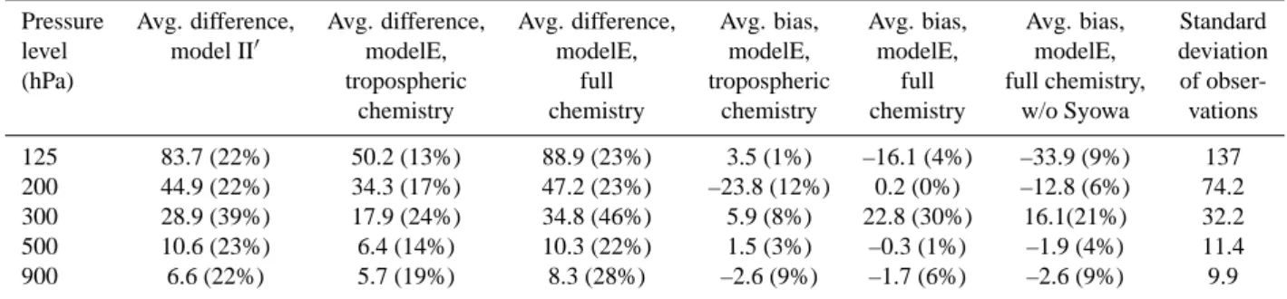
Table 4. Ozone differences and biases (ppbv) between models and sondes.

Pressure Avg. difference, Avg. difference, Avg. difference, Avg. bias, Avg. bias, Avg. bias, Standard

level model II0 modelE, modelE, modelE, modelE, modelE, deviation

(hPa) tropospheric full tropospheric full full chemistry, of

obser-chemistry chemistry chemistry chemistry w/o Syowa vations

125 83.7 (22%) 50.2 (13%) 88.9 (23%) 3.5 (1%) –16.1 (4%) –33.9 (9%) 137

200 44.9 (22%) 34.3 (17%) 47.2 (23%) –23.8 (12%) 0.2 (0%) –12.8 (6%) 74.2

300 28.9 (39%) 17.9 (24%) 34.8 (46%) 5.9 (8%) 22.8 (30%) 16.1(21%) 32.2

500 10.6 (23%) 6.4 (14%) 10.3 (22%) 1.5 (3%) –0.3 (1%) –1.9 (4%) 11.4

900 6.6 (22%) 5.7 (19%) 8.3 (28%) –2.6 (9%) –1.7 (6%) –2.6 (9%) 9.9

Comparisons are between the models and the 16 recommended sites of Logan (1999), having excluded the two sites with four months or less data. Average differences are a simple average of the month-by-month absolute value differences between the model and the sondes. Average biases are averages of the model-sonde differences without first taking the absolute value. Numbers in parentheses are percent difference with respect to observed values at these levels. The sites are: Resolute, Edmonton, Hohenpeissenberg, Sapporo, Boulder, Wallops Island, Tateno, Kagoshima, Naha, Hilo, Natal, Samoa, Pretoria, Aspendale, Lauder, and Syowa. All models are 23 layer versions.

especially down into the troposphere. However, the values in the troposphere and near the tropopause in general are all more negative in the model since these simulations did not in-clude increases in tropospheric ozone precursors. As seen in runs that did include such increases, the troposphere became more and more polluted during the twentieth century, which would account for the positive trends seen in the lowermost portion of the SAGE data at mid-latitudes and in the tropics and also the smaller negative values seen at high latitudes.

To evaluate the lowermost stratosphere and troposphere, where satellite climatologies do not yet exist, we have exten-sively compared modeled annual cycles of ozone with a long-term balloon sonde climatology from remote sites (Logan, 1999). Annual cycles at several pressure levels are shown for selected sites in Fig. 7, while statistical comparisons with all sites are presented in Table 4. Results are included for sim-ulations incorporating chemistry throughout the model do-main and for simulations with tropospheric chemistry only. Values from the previous model II0version are also shown in the table for comparison.

The ozone values and annual cycles over a wide range of latitudes are reasonably well simulated (Fig. 7). The high lat-itude biases evident in the previous analysis of the total col-umn are immediately apparent at the uppermost sonde lev-els, however. The full chemistry version underpredicts win-tertime ozone at 125 hPa at both Resolute and Hohenpeis-senberg, and overpredicts at Lauder and especially at Syowa. The biases have only a minor effect on lower altitudes at most locations, with the exception of Syowa where they persist clearly through at least 500 hPa. The shape of the seasonal cycle is generally well reproduced in the model, with max-imum and minmax-imum values typically falling at the correct time of year. There is clearly an underestimate of ozone in the tropical upper troposphere at Natal, but this is not the case at other locations.

A broader comparison of all 16 ozonesonde sites, as shown in Table 4, demonstrates that the new composition and cli-mate model gives a substantially improved simulation in comparison with the older model II0tropospheric chemistry model. Running the new model in tropospheric chemistry-only mode leads to a better match with observations at all levels, though especially those away from the surface. Using the full chemistry calculation, inherently a more difficult en-deavor compared with prescribing stratospheric ozone to ex-actly match observations, coincidentally leads to differences with respect to observations that are quite similar to those seen in the tropospheric chemistry-only model II0. However, this implies that at a level such as 125 hPa, in the stratosphere for many of the sites, the full chemistry model does a much better job for the low latitude sites for which this level is in the troposphere (consistent with the modelE tropospheric chemistry-only performance).

Transport from the stratosphere to the troposphere is sub-stantially improved in the new modelE, as evidenced by the improvement in the tropospheric chemistry modelE ver-sus II0. Thus the large positive bias in the full chemistry model at 300 hPa does not result solely from excessive down-ward transport, a major problem in previous GISS GCMs. It is at least partially attributable to the overestimate of high latitude lower stratospheric ozone, especially in the SH. A similar statistical comparison of the full chemistry run with sonde data leaving out the two high latitude sites Resolute and Syowa shows average differences in ppbv reduced from 34.7 to 23.7 at 300 hPa, from 45.7 to 37.0 at 200 hPa, and from 83.2 to 75.8 ppbv at 125 hPa, while at lower levels, there is little effect. This demonstrates that, as expected, a fair amount of the discrepancy with observations arises from the model’s high latitude biases. However, some excessive downward transport may still be occurring, which is par-tially masked in the tropospheric chemistry-only run by the negative bias at 200 hPa. The large 300 hPa positive bias is

(13)

1 2 3 4 5 6 7 8 9 10 11 12 200 400 600 800 1000 1200 1400 1600 1800 Resolute (75 N), 125 hPa Month 1 2 3 4 5 6 7 8 9 10 11 12 100 250 400 550 700 850 1000 1150 Hohenpeissenberg (48 N), 125 hPa Month 1 2 3 4 5 6 7 8 9 10 11 12 0 50 100 150 200 250 300 350 Hilo (20 N), 125hPa Month 1 2 3 4 5 6 7 8 9 10 11 12 0 100 200 300 400 500 600 700 800 900 200 hPa Month 1 2 3 4 5 6 7 8 9 10 11 12 0 100 200 300 400 500 600 200 hPa Month 1 2 3 4 5 6 7 8 9 10 11 12 0 25 50 75 100 125 150 200 hPa Month 1 2 3 4 5 6 7 8 9 10 11 12 0 100 200 300 400 300 hPa Month 1 2 3 4 5 6 7 8 9 10 11 12 0 50 100 150 200 300 hPa Month 1 2 3 4 5 6 7 8 9 10 11 12 0 25 50 75 100 125 150 300 hPa Month 1 2 3 4 5 6 7 8 9 10 11 12 0 25 50 75 100 500 hPa Month 1 2 3 4 5 6 7 8 9 10 11 12 0 25 50 75 100 500 hPa Month 1 2 3 4 5 6 7 8 9 10 11 12 0 25 50 75 100 500 hPa Month 1 2 3 4 5 6 7 8 9 10 11 12 0 25 50 900 hPa Ozone (ppbv) Month 1 2 3 4 5 6 7 8 9 10 11 12 0 25 50 900 hPa Ozone (ppbv) Month 1 2 3 4 5 6 7 8 9 10 11 12 0 25 50 900 hPa Ozone (ppbv) Month

Fig. 7. Comparison of ozone’s annual cycle in the model with an ozonesonde climatology (Logan, 1999) at the given locations and pressure levels. Solid lines give observed mean values, while filled circles and open triangles show results from the tropospheric chemistry-only and full chemistry simulations, respectively. Model values have been interpolated onto the given pressure levels.

(14)

1 2 3 4 5 6 7 8 9 10 11 12 0 25 50 75 100 125 150 175 200 Natal (6S), 125 hPa Month 1 2 3 4 5 6 7 8 9 10 11 12 0 100 200 300 400 500 600 700 800 Lauder (45S), 125 hPa Month 1 2 3 4 5 6 7 8 9 10 11 12 100 200 300 400 500 600 700 800 900 1000 Syowa (69S), 125 hPa Month 1 2 3 4 5 6 7 8 9 10 11 12 0 50 100 150 200 200 hPa Month 1 2 3 4 5 6 7 8 9 10 11 12 0 100 200 300 400 500 200 hPa Month 1 2 3 4 5 6 7 8 9 10 11 12 0 100 200 300 400 500 200 hPa Month 1 2 3 4 5 6 7 8 9 10 11 12 0 25 50 75 100 125 150 300 hPa Month 1 2 3 4 5 6 7 8 9 10 11 12 0 25 50 75 100 125 150 300 hPa Month 1 2 3 4 5 6 7 8 9 10 11 12 0 50 100 150 200 300 hPa Month 1 2 3 4 5 6 7 8 9 10 11 12 0 25 50 75 100 500 hPa Month 1 2 3 4 5 6 7 8 9 10 11 12 0 25 50 75 100 500 hPa Month 1 2 3 4 5 6 7 8 9 10 11 12 0 25 50 75 100 500 hPa Month 1 2 3 4 5 6 7 8 9 10 11 12 0 10 20 30 40 50 900 hPa Ozone (ppbv) Month 1 2 3 4 5 6 7 8 9 10 11 12 0 10 20 30 40 50 900 hPa Ozone (ppbv) Month 1 2 3 4 5 6 7 8 9 10 11 12 0 10 20 30 40 50 900 hPa Ozone (ppbv) Month Fig. 7. Continued.

(15)

1 2 3 4 5 6 7 8 9 10 11 12 0 10 20 30 40 50 60