Dynamics of long flexible cylinders at high-mode number in uniform and sheared flows

(1)

Dynamics of Long Flexible Cylinders at High-Mode Number in Uniform and Sheared Flows

by

Susan B. Swithenbank

B.S. Mechanical Engineering (2000) Carnegie Mellon University

Submitted to the Department of Mechanical Engineering in Partial Fulfillment of the Requirements for the Degree of

Doctor of Philosophy in Ocean Engineering at the

Massachusetts Institute of Technology February 2007

Signature of Author……… Department of Mechanical Engineering January 30, 2007

Certified by……… J. Kim Vandiver Professor of Mechanical and Ocean Engineering Thesis Supervisor

Accepted by………... Lallit Anand Chairman, Department Committee on Graduate Students

(2)

Dynamics of Long Flexible Cylinders at High-Mode Number in Uniform and Sheared Flows

By

Susan B. Swithenbank

Submitted to the Department of Mechanical Engineering on January 30, 2007 in partial fulfillment of the requirements for the Degree of Doctor of Philosophy in

Ocean Engineering ABSTRACT

The primary objective of this thesis is to characterize the response of risers at high-mode numbers in sheared and uniform ocean currents. As part of this thesis work, three separate experiments have been planned and executed. The objective of these tests was to create a set of model tests at high-mode numbers, the first test was in uniform currents and the other tests in sheared currents.

In the experiments, Vortex-Induced Vibrations (VIV) happened at one frequency at one time, rather than at many frequencies simultaneously. The single VIV frequency varied with time, but the VIV frequencies did not co-exist. The major impact of time-sharing frequencies is that it increases the damage rate and fatigue of the pipe.

The high density of the sensors on the pipe allowed for analysis that had not previously been done. Two methodologies are presented to locate the area of the power-in region. Once the region where the vibration originated has been found, the different phenomena that effect the location of the power-in region that were discovered are shown. Four different factors are presented that effect the locations of the power-in region: the incidence angle of the current, the gradient of the current direction, the current profile, and the end effects at high mode number.

Two dimensionless parameters are presented which help in the prediction of VIV given a current profile. The first is the power-in determination factor which predicts the region where the power-in occurs using a combination of the current velocity and the power-in length. The second parameter, the time sharing parameter, helps to determine whether the riser will respond with a single frequency, or switch between frequencies in time.

Thesis Supervisor: J. Kim Vandiver

(3)

Chapter 1: Introduction

Vortex-induced vibrations (VIV) have been a long standing problem for mooring lines and drilling risers in ocean-current fields. During the last 20 years, the prediction of VIV has greatly improved by using data collected in laboratory tests and information from risers in the field. Multiple VIV prediction programs have been written to help engineers predict VIV and help in the design of future underwater applications.

The natural resources that are being developed today are in deeper water with stronger currents. The design with respect to VIV becomes more important because of the increased risk of fatigue failure.

Present modeling programs were designed and proven using data on shorter risers and from laboratory experiments at low-mode numbers. With the move from risers in shallow water to those in deep water comes the need to validate these programs at high-mode number.

The objectives of this thesis are four-fold:

• Help design and complete a set of tests to investigate VIV at high-mode numbers in uniform and sheared flow

• Determine when single-frequency and multi-frequency VIV responses are observed

• Define dimensionless parameters to help predict the dynamics of long cylinders at high-mode numbers

• Determine under what conditions of current shear separable cross-flow and in-line responses are observed

In the last two years, three separate scaled-model tests have been designed and completed by Prof. Vandiver’s research group to investigate high-mode number VIV: two Miami Gulf Stream Tests and the Lake Seneca Test.

The first test was conducted at the Naval Acoustic Test Facility at Lake Seneca, New York. The Lake Seneca facility presented a controlled environment where uniform flow velocity and uni-directional cases could be investigated. At Lake Seneca a 400 ft long pipe with a diameter of 1.3 inches was instrumented with 25 tri-axial accelerometers to measure the VIV.

(7)

The Lake Seneca experiment was a controlled experiment conducted in a lake. The flow was virtually uniform over the span of the pipe, and the direction of the current was known. The in-line and cross-flow responses are evident in both the amplitude and the spectrum of the cases at Lake Seneca.

In comparison, the second and third tests, which were conducted in the Gulf Stream off the coast of Miami, had sheared currents and multi-directional flow. The Gulf Stream allowed for a greater variety of current profiles. Different types of sheared currents were seen in the Gulf Stream. In the two Miami experiments, an approximately 500 ft long pipe was instrumented with 70 fiber optic strain gauges in each of four quadrants.

The tests were designed to produce responses at high-mode numbers. The model was scaled so that high-mode numbers would be excited, where high-mode numbers are defined as those greater than the 10th mode.

Results

The results of the four objectives are shown in different chapters throughout the thesis. The test design and results from the tests are shown in Chapter 3 and Appendix G. Chapter 3 shows the overall test design, whereas Appendix G shows the accelerometer placement algorithm in detail.

In the experiments, Vortex-Induced Vibrations (VIV) happened at one frequency at one time, rather than at many frequencies simultaneously. The single VIV frequency varied with time, but the VIV frequencies did not co-exist. The major impact of time-sharing frequencies is the impact upon the damage rate and fatigue of the pipe. The discussion of time-sharing of frequencies is presented in Chapter 5.

Chapter 6 presents two methodologies for finding the source of the VIV. One methodology is based on the reduced velocity and has been used before. The second methodology uses the signal processing technique called coherence to locate the source of the vibrations.

Using the results of the techniques discussed in Chapter 6, the effects of different factors on the location of the source region were examined. Factors such as the angle of incidence of the current, the gradient of the current direction, the reduced velocity

(8)

bandwidth and the proximity to the boundary were all factors in where the source region was located.

Chapter 9 presents the derivation of two dimensionless parameters that help predict the behavior of cylinders at high-mode numbers. The first parameter predicts the center of the source region. The second parameter determines whether the vibrations will be single frequency or switch between frequencies.

(9)

Chapter 2: Test Description

Introduction

The tests at Lake Seneca were conducted in the summer of 2004 and focused on the measurement of VIV in uniform flow at high-mode number for a bare pipe and for the same pipe with complete strake coverage. In comparison, the Gulf Stream tests were conducted in October 2004 and October 2006 and focused on bare pipe, partial strake coverage, and partial fairing coverage with sheared flow. Both tests are part of a larger VIV-testing program developed by DEEPSTAR, a joint industry technology development consortium.

As oil exploration and drilling moves into deeper water, understanding the dynamics of long pipes, vibrating at high mode numbers in sheared currents, becomes important. Additionally, understanding how strakes affect the dynamics of bare pipe is also important. The main objectives of the Gulf Stream Test were:

• To gather vortex-induced vibration response data using a densely instrumented circular pipe at high-mode numbers

• To measure mean drag coefficients (CD) at high-mode numbers and

improve drag-coefficient prediction formulas.

• To test the efficacy of helical strakes at high-mode numbers.

• To obtain statistics on the distribution of single-mode vs. multi-mode response to VIV.

• To determine the relative contribution to damage rate, arising from in-line and cross-flow VIV.

• To improve knowledge of damping factors on risers equipped with helical strakes.

Lake Seneca Experiment Description

The Lake Seneca test facility was selected as the testing site, because it is a fully equipped field-test station moored in calm, deep water. It was ideal for conducting a controlled test on a long circular pipe in uniform flow. This was accomplished by towing a vertical, composite pipe with a suspended bottom weight to produce the desired tension.

The length, diameter, and tension of the pipe were chosen so as to permit cross-flow excitation of up to the 25th mode. The maximum speed possible with the system at Lake Seneca was limited by the maximum allowable deflection angle of the pipe. Typical

(10)

towing speeds were approximately 1.0 to 3.5 ft/s, (0.3 to 1.1m/s). Vandiver and Marcollo, [2003], provide an analysis of the design tradeoffs when attempting to achieve high-mode numbers. This is done in terms of tension, length, diameter, and top angle.

The pipe was constructed in 100 foot segments which were then joined together. The depth of Lake Seneca limited the total pipe length to a maximum of 450 ft. During the experiment, total lengths of 201 and 401 feet (61.26 and 122.23 m) were tested. The properties of the pipe are shown in Table 1.

Table 1- Mechanical Properties of the Fiberglass Model Riser Used in the Lake Seneca Tests

Outer diameter 1.310 in.(0.0333m)

Inner diameter including liner 0.980 in.(0.0249m)

Lengths tested 201 & 401 feet(61.26 & 122.23m)

Effective tension 805 lbs submerged bottom weight (3581N) Modulus of elasticity (E) 1805.0 ksi (1.276E10 N/sq m)

Moment of inertia (I) 3.994E-06 ft4 (3.447E-8 m4)

EI 149489.3 [lb-in2](429.0 N-m2)

Mass / displaced mass of water 1.35

Weight per unit length in air 0.79 [lb/ft](11.53 N/m),(1.176 kg/m)

Each 100 foot long section of pipe contained six evenly spaced tri-axial accelerometers. These accelerometers were sampled by analog-to-digital converters and micro-processors located locally at each accelerometer unit. The units were connected to a digital serial network, which had two parallel branches for redundancy. Half of the accelerometers used one network branch and half used the other. In this way, if one branch failed, half of the data would still be retrieved. The networks were controlled by a surface computer, which set the sampling rate and downloaded the data from each accelerometer unit. The surface data acquisition system was designed and built by BMT Scientific Marine Services Inc.

The sampling rate used in these experiments was 60 Hz for every accelerometer. The same serial network was used to sample the tension and tilt-measuring devices located very close to the top universal-joint connection.

Towing speed was measured by two mechanical current meters. One was suspended underneath the towed weight and the other was hung over the side of the towing vessel. The current meters were cup anemometer devices, with a magnetically activated reed switch which detected the rotation of the spinning multi-cup rotor. One

(11)

pair of wires ran the full length of the pipe from the bottom current meter to the data acquisition system on the surface.

In total, the pipe had ten conductors of wires which ran the full length. Two pairs of wires were used to support the serial networks. One pair carried power to all accelerometers. One pair was used for the bottom current meter and one pair was a spare. A ten-conductor waterproof connector was made up between each 100-foot long pipe section. The pipe was filled with a flexible epoxy compound to exclude water and to hold the wires in place.

At the top of the pipe, a load cell and tilt meter were attached. This additional instrumentation allowed the measurement of the tension in the pipe and the top angle of inclination.

The experimental set-up can be seen in Figure 1.

Figure 1 - Experimental Setup

The pipe was first assembled and deployed using a crane on the moored barge in Lake Seneca. The pipe was then transferred by crane from the perch on the barge to a perch on the bow of a supply boat. The supply boat was driven in reverse. In reverse, the slow speeds needed for the experiment could be more easily controlled. A railroad wheel

Boat Pipe Railroad Wheel Current Current Meter Tilt Meter Current Meter Load Cell Perch Fin Accelerometers

(12)

was connected to the bottom end to provide tension. Fins mounted on the railroad wheel prevented it from pitching and rotating. Great care was taken to design the towed weight so that it would have dynamic-response characteristics which would not interfere with the desired VIV. In particular, the pitch and roll natural frequencies of the weight were approximately 0.8 Hz and lower than the lowest VIV response frequency of interest. Accelerometer Design

The placement of instrumentation on a riser can be crucial to later analysis of the data. If the sensors are not placed correctly, certain types of analysis such as modal analysis are impossible. With incorrectly placed instruments, the modes could be misidentified as other modes through aliasing, or missed entirely. The purpose of the sensor placement algorithm is to find the optimal placement for instrumentation on a riser that will avoid these problems.

An algorithm for placement is shown in Appendix G; this algorithm of the placement of sensors uses assumed mode shapes. Since mode shapes are orthogonal, the dot product of any two different modes should be zero. In the case of an instrumented riser, the mode shapes are discretely sampled only at the locations of the instrumentation. If the sampling of the mode shapes is poorly chosen, then the dot product of two different modes will not be zero. This algorithm considers the dot product of all the mode shapes when discretely sampled at the specified sensor locations and tries to minimize the dot products by locating the sensors in the optimal position.

Gulf Stream Test Description

The 2004 Gulf Stream test was conducted on the Research Vessel F. G. Walton Smith, operated by the University of Miami. The composite pipe was 485.3 feet long and 1.4 inches in diameter. The pipe was instrumented with embedded fiber optic strain gauges to monitor the vibration.

The 2006 Gulf Stream test was also conducted on the Research Vessel F. G. Walton Smith, operated by the University of Miami. The composite pipe was 504.5 feet long and 1.41 inches in diameter. The pipe was also instrumented with embedded fiber optic strain gauges to monitor the vibration. The experiment setup is show in Figure 2.

(13)

For both tests, the pipe was spooled on a drum that was mounted on the aft portion of the boat. The pipe was un-spooled and lowered into the water using a hydraulic motor. At the bottom end was a railroad wheel assembly which included a current meter, a center spool and U-joint. The assembly weighed 836 lbs in air and approximately 725 lbs in water, and was attached to the bottom of the pipe to provide tension. The weight of the pipe in water was 0.12 lb/ft. With additional drag forces on the pipe, the mean total top-end tension was 820 lb. The pipe was attached to the stern of the boat on a perch. About six feet of pipe were above the waterline. A variety of current profiles with significant variation in speed and direction were achieved by steering the vessel at numerous headings, while in the Gulf Stream.

Current Meter Current Meter Pipe Railroad Wheel F. G. WALTON SMITH Spooler

Load Cell and Tiltmeter

Fin Current Meter Current Meter Pipe Railroad Wheel F. G. WALTON SMITH Spooler

Load Cell and Tiltmeter

Fin

Figure 2 – Experiment setup for the Gulf Stream Test

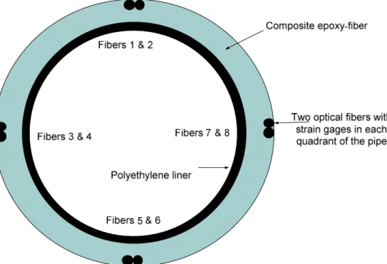
Eight optical fibers were embedded under the outer layer of the pipe during manufacture. Each fiber contained 35 strain gauges, spaced fourteen feet apart. Two fibers were located in each of the four quadrants of the pipe, as see in Figure 3.

(14)

Figure 3 - Cross-Section of the Pipe from the Gulf Stream Test

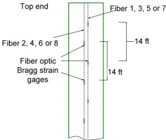
The gauges in one fiber of a pair were not placed at the same axial position as the gauges in the adjacent fiber. Instead they were offset axially from one another by seven feet, as seen in Figure 4. When both fibers are functioning, a spatial resolution of seven feet was achieved. By merging the data from both fibers, an effective resolution was achieved with seventy total strain gauges per quadrant.

During the experiments, the exact orientation of the four quadrants was not known. This is due in part to a residual twist over the total length of the pipe of approximately 60 degrees, which was introduced in the fabrication process. There was a fin on the wheel, which was intended to orient the wheel in the current. However, the exact current direction at the wheel is not known because the depth of the wheel varies with changes in the drag force. It is known that within the same quadrant, the orientation of the optical fibers varies slowly. The conclusions reached in this paper do not depend on knowing the exact orientation of the strain gauges with respect to the boat. This is not a significant limitation in understanding the efficacy of strakes. It will be shown that there is very little difference in RMS amplitude and frequency content between gauges located in different quadrants.

(15)

Figure 4 - Side View of the Pipe from the Gulf Stream Test

The pipe properties are found in Table 2 for the 2004 experiment and Table 3 for the 2006 experiment.

Table 2 –2004 Gulf Stream Pipe Properties

Inner diameter 1.05 in. (0.0267 m)

Outer diameter 1.40 in.(0.0356 m)

Optical fiber diameter 1.30 in.(0.033 m)

EI 1.7e5 lb.in2 (488 Nm2)

Modulus of elasticity (E) 2.30e6 lb./in2 (1.586e10 N/m2)

EA 8.5e5 lb. (3.78e6 N)

Weight in seawater 0.12 lb./ft. (flooded in Seawater) (1.75 N/m)

Weight in air, w/trapped water 0.83 lb./ft. (12.11 N/m)

Density 0.053 lb/in3 (1.47 g./cc).

Material Carbon fiber –epoxy

Length 485.3 ft (147.3 m) (U-joint to U-joint)

Roughness (k/D) 0.002

Table 3 – 2006 Gulf Stream Pipe Properties

Inner Diameter 0.98 inch (0.0249 m)

Outer Diameter 1.43 inch (0.0363 m)

EI 1.483e3 lb ft2 (613 N m2) EA 7.468e5 lb (3.322e6) Weight in Seawater 0.1325 lb/ft (0.1972 kg/m) Weight in air 0.511 lb/ft (0.760 kg/m) Density 86.39 lb/ft3 (1383 kg/m3) Effective Tension 725 lb

(16)

Length 500.4 ft (152.524 m)

Manufactured by FiberSpar Inc

An Acoustic Doppler Current Profiler (ADCP) was used to record the current along the length of the pipe. An ADCP uses acoustic sound waves to measure current speed and direction. The ADCP sends out an acoustic ping and waits for the return sound. Based on the time the ping takes to return and the Doppler shift in frequency, the ADCP obtains an estimate of the current speed as a function of depth.

The R/V F. G. Walton Smith has high and low frequency ADCPs. The broadband (600 kHz) ADCP is used to obtain a greater resolution and accuracy at the shallow depths, whereas the narrowband (150 kHz) ADCP is used for deeper depths. During the Gulf Stream testing both ADCPs were used to gather data.

Additional instrumentation included a tilt meter to measure the inclination of the top of the pipe, a load cell to measure the tension at the top of the pipe, and two mechanical current meters to measure current speed at the top and the bottom of the pipe. Strake Properties

The strakes, used for both the Lake Seneca and the Gulf Stream experiments, were of a triple helix design made of polyethylene, with a pitch of 17.5 times the diameter of the pipe. This represents a typical design for strakes in the industry. The properties of the strakes are shown in Table 4. The strakes had a slit down the side that allowed them to be snapped over the outside of the pipe, and secured to the pipe using tie wraps. The strakes were manufactured by AIMS International.

Table 4 - Strake Properties

Material Polyethylene

Length 26.075 in. (0.66 m)

Shell OD 1.49 in.(0.038 m), includes the strake height Shell ID 1.32 in. (0.0335 m)

Strake height 0.375 in. (0.009 m) (about 25% of shell diameter) Wall thickness 0.09 in.(0.0022 m)

Pitch 17.5 times the Diameter

(17)

Figure 5 - Strakes Attached to the Pipe at Lake Seneca Fairing Properties

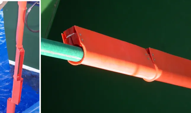
A new fairing, designed and fabricated by AIMS International, was tested. The properties of the fairings are shown in Figure 6. The fairings used a split design, which allowed them to be snapped over the outside of the pipe, and were secured to the pipe using rubber bands (Figure 6). The fairings were attached in groups of five. Between each group a thrust collar was attached to the pipe with a tie wrap. The collar prevented the fairing from sliding up or down the pipe, which could have caused the fairings to interfere with free rotation and alignment. The fairings were manufactured and donated by AIMS International.

Table 5 - Fairing Properties

Material Polyethylene

Length(inches) 14.96 in (38 cm)

Shell Thickness (inches) 0.132 in (3.35 mm) Shell ID(inches) 1.38 in (3.51 mm) Weight/length in air(lbs/ft) 0.764 lb (0.341 g) Length of Fairings (in/mm) 9.15 in (3.6 mm)

(18)

Figure 6 - Fairings attached to pipe during the second Gulf Stream experiment Results from Lake Seneca

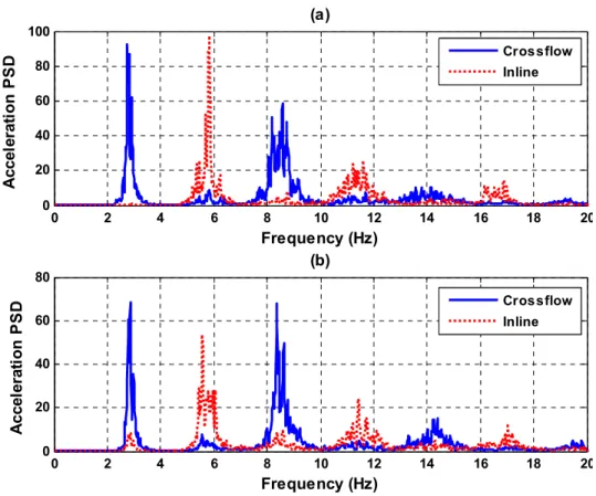
As stated above, the current profiles at Lake Seneca were essentially uniform with the only variation caused by the angle of the pipe with the vertical. Figure 7 shows the cross-flow acceleration Power Spectral Density (PSD) for a Lake Seneca test. The PSDs in the figure correspond to points located at 75 ft (x/L = 0.19) and 309 ft (x/L = 0.77) from the top end. The odd harmonics were seen in the cross-flow spectrum while the in-line spectrum captures the even harmonics. As mentioned earlier, this paper focuses on the cross-flow components and therefore the odd harmonics.

The PSD of the acceleration response at Lake Seneca shows that the frequency content was sharply peaked, indicating that the excitation was a quite narrow band at the fundamental excitation frequency. Although the magnitudes of the PSDs at the two different locations were different, the frequency content was the same at both points, indicating that the same fundamental VIV frequency was excited along the whole length of the pipe. Figure 7 also shows that there was significant energy in the cross-flow spectrum at the three-time frequency. The three-time harmonic is consistent with the results of Jauvtis and Williamson [2004].

(19)

0 2 4 6 8 10 12 14 16 18 20 0 20 40 60 80 100 A c c e le ra ti o n P S D Frequency (Hz) (a) Crossflow Inline 0 2 4 6 8 10 12 14 16 18 20 0 20 40 60 80 A c c e le ra ti o n P S D Frequency (Hz) (b) Crossflow Inline

Figure 7 – Cross-flow and in-line acceleration PSDs showing the lack of spatial variation in

frequency content in the Lake Seneca experiments. 1.76 ft/s = Un, 5.5 = Vr, (a) At x/L = 0.19 from top

end, (b) At x/L = 0.77 from top end. The units of both (a) and (b) are (m/s2)2/Hz Results from the 2004 Gulf Stream Test

An example comparing the different tests scenarios and strake configurations from the Gulf Stream tests is shown in Figure 8. One test case from each of the test configurations is shown: bare, 40% coverage at the bottom, and 70% staggered coverage. The cases were chosen to have similar current profiles so the results can be more easily compared. In the cases shown, the stronger currents are at the bottom of the pipe. The sheared profiles vary from approximately 2.4 ft/s to 3.2 ft/s.

Figure 9 shows the RMS strain measured for the second quadrant for each of the three strake configurations. The total strain as measured at any strain gauge is made up of contributions from bending as well as tension variations in the test pipe. To estimate true bending strain, one must subtract in the time domain the strain measured in one quadrant from that measured in the quadrant on the opposite side of the pipe. This computation results in common tension contributions in both fibers canceling one another, but allows common bending strains to add.

(20)

Figure 8 - Current Profiles for Comparison of the Bare Pipe Response to that with 40% and 70% Strake Coverage 50 100 150 200 250 300 -500 -450 -400 -350 -300 -250 -200 -150 -100 -50 0 RMS Strain µµµεεεεµ D e p th ( ft ) Bare 40% Strakes Staggered Strakes

Figure 9 - RMS Strain in the Second Quadrant for Pipe with and without Strakes

In this study, fiber optic-mechanical failures greatly reduced the number of paired strained gauges, which were on opposite sides of the pipe. It was rarely possible to

2.2 2.4 2.6 2.8 3 3.2 3.4 3.6 3.8 -500 -450 -400 -350 -300 -250 -200 -150 -100 -50 0 Current (ft/s) D e p th ( ft ) Bare 40% Strakes Staggered Strakes

(21)

evaluate true bending. In order to salvage useful information from single-fiber measurements, the data was filtered to eliminate the low-frequency tension variations caused by vessel motion. Vessel heave, pitch and roll periods were in excess of 2 seconds and waves large enough to affect vessel motion had periods in excess of three seconds. In order to isolate bending energy from the tension variations due to vessel motion, the data was high pass filtered at 1.0 Hz. VIV frequencies of interest were at 2 Hz and above. All data shown here has been high pass filtered.

Most of the dynamic strain data presented in this paper has been extracted from single-gauge measurements because, due to fiber failures, it was frequently not possible to take the difference between measurements from strain gauges on opposite sides of the pipe. Though disappointing, this was not entirely unexpected. The use of fiber-optic strain gauges in this application was pushing the state of the art in the use of such gauges. A significant amount of valuable data was obtained, including gaining experience with a new measurement technology.

When comparing the RMS strain from a single fiber for the various coverage scenarios the bare case has the highest response, as expected.

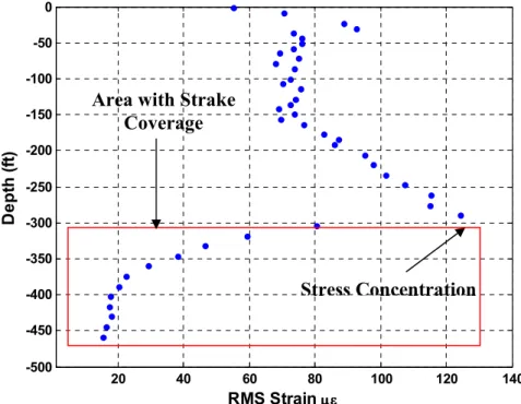
The case with 40% strake coverage shows the previously described stress concentration at the point of reflection. For this particular case, the RMS single-fiber strain is about half the RMS single-fiber strain for the bare case at all locations, including the point of the stress concentration. The RMS single-fiber strain for the staggered strake coverage is less than one-fifth that of the bare coverage case, and does not exceed 50 micro-strain (µε) at any point on the pipe. The stress concentration is highlighted in Figure 10.

(22)

20 40 60 80 100 120 140 -500 -450 -400 -350 -300 -250 -200 -150 -100 -50 0 RMS Strain µµµεεεεµ D e p th ( ft )

Figure 10 – RMS strain from 40% strake coverage at the bottom showing the stress concentration at 300 ft below the top universal joint.

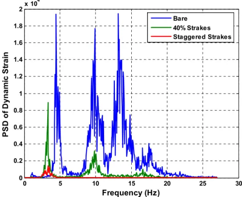
The impact of the strakes can be seen not only in a reduction of RMS strain, but also in a change in frequency content. Figure 11 shows the PSD for each of the different strake configurations at an axial position 306 feet from the top. This depth is just inside the region with strakes in the 40% case and is in a region without strakes for the 70% strake coverage case.

The dominant VIV frequency for the bare case (the blue curve in Figure 11) is 4.48 Hz. There is also a prominent two-time harmonic peak and a broad peak which includes significant energy at three-time the dominant VIV frequency.

The dominant VIV frequency for the 40% straked coverage case is 3.32 Hz. This is the green curve in Figure 11. There is also a small three-time peak. The frequency content of the response is changed by the strakes. The bare pipe case contains frequencies up to 25 Hz with significant energy up to 20 Hz. When 40% strakes are applied, the frequency content is limited to approximately 20Hz with significant energy up to 12 Hz. With 70% staggered strake coverage, the frequency content of the pipe is limited to 6 Hz at the location of this strain gauge with no visible two-time and three-time components.

Stress Concentration Area with Strake

(23)

Figure 11 - PSD of the three configurations at 306 feet from the top 0 5 10 15 20 25 30 0 0.2 0.4 0.6 0.8 1 1.2 1.4 1.6 1.8 2x 10 4 Frequency (Hz) P S D o f D y n a m ic S tr a in Bare 40% Strakes Staggered Strakes

(24)

Chapter 3: Literature Review

Introduction

This chapter introduces important parameters that affect Vortex-Induced Vibrations (VIV). Various parameters control whether or not VIV cause large-amplitude vibrations that could fatigue a structure. The parameters are both structural and hydrodynamic. Flow around a Cylinder

When flow passes a bluff body, such as a cylinder, the boundary layer on both sides of the cylinder separates, creating two shear layers that bound the wake. Within the shear layer, the flow at the surface of the structure approaches zero velocity, forming vortices in the wake of the cylinder. These vortices, formed by the separating shear layer, are periodic and apply forces on the cylinder. Figure 12 shows the vortex-wake pattern for a cylinder in laminar flow.

Figure 12 – Vortex-wake pattern from an oscillating cylinder [Griffen and Ramberg 1974]

The frequency with which vortices shed is a function of the current velocity, U. One parameter used to characterize vortex shedding from stationary cylinders is the Strouhal number:

(25)

n f D St

U

= (3.1)

where U is the free stream current velocity, D is the diameter, and fn is the natural

frequency of the nth mode.

The Reynolds number is important in VIV. The vortex wake changes depending on the Reynolds number, defined as:

Re UD

ν

= (3.2)

where ν is the kinematic viscosity of the fluid.

Figure 13 shows the relationship between the Strouhal number and the Reynolds Number as shown for a stationary cylinder [Blevins, 2001].

Figure 13 –The Relationship between Strouhal Number and Reynolds Number, [Blevins 2001] The vortex shedding wake responds differently depending on the regime that the Reynolds number is in. Laminar flow is from a Reynolds number of 0 to ~350. Sub-critical turbulent flow happens at Reynolds numbers from ~350 to ~100k. The Sub-critical regime is from ~100k to ~6M. The super-critical regime is Reynolds numbers greater than 6M. Vortex shedding can happen in all the regimes of the Reynolds number, but the pattern of the shedding will differ.

(26)

The roughness of the pipe can vary the Reynolds number governing the transition from sub-critical to critical. The rougher the pipe, the lower the Reynolds number needed to enter the critical regime. [Achenbach and Heinecke 1981]

For most offshore platforms, the Reynolds number is in the critical regime (~100k < Re < 6M). The Lake Seneca and Gulf Stream experiments were in the sub-critical regime (~350 < Re < ~100k).

When discussing vibrating cylinders, a second parameter called the reduced velocity is often used instead of the Strouhal number. The reduced velocity can be defined two different ways. The first is:

n r v U V f D = (3.3)

where fv is the frequency of vibration.

Additionally the reduced velocity can be defined as n rn n U V f D = (3.4)

where fn is the natural frequency of the cylinder at a specific condition .

The main difference between Vr and Vrn is that the frequency of vibration can be

any range of frequencies depending on the current, whereas the natural frequency, as used in Vrn, is a fixed value.

Vortices can be shed at any reduced velocity, but the amplitude of vibration is often dependant on the value of the reduced velocity. At reduced velocities of less than four, few vibrations are seen. The largest amplitude of vibrations is seen at reduced velocity of 5 < Vr < 7 for sub-critical Reynolds numbers. .

Normal-Incident Current

The setup of the Gulf Stream and Lake Seneca tests had the top end of the pipe inclined due to drag force. Since the pipe is inclined, the current is not normal to the pipe. This inclination angle is important when considering the vibrations. Only the component that is normal to the pipe is considered when calculating vibration of the pipe. Figure 14 shows the current divided into normal and tangential component vectors.

Therefore: cos n

(27)

where Φ is the incidence angle of the pipe with the vertical.

For the Gulf Stream tests, the inclination angle can be as great at 60°. This can reduce the current by up to 50%.

Figure 14 - The pipe showing normal incident current Speed of Propagation and Natural Frequency

The speed of propagation and the natural frequency are proportional. With the speed of propagation equal to:

c= fλ (3.6)

a pipe under tension has a speed of propagation that may be frequency dependant. At low frequencies, the pipe is dominated by tension effects and reacts like a tensioned string with a constant speed of propagation of:

T c m = (3.7)

Current (U)

U

t

U

n

Φ

(28)

where c is the speed of propagation, T is the tension, and m is the mass per unit length including the added mass.

At high frequencies, the speed of propagation is controlled by the bending stiffness of the pipe. The speed of propagation therefore is:

2 EI

c

m

ω

= (3.8)

where E is the Young’s modulus, I the moment of inertia, and A is the cross-sectional area.

In between, the pipe will react as a combination of the tensioned string and the beam with pinned-pinned connections. The speed of propagation is:

1 2 2 T n EI c m L m π  _ _  =_ +_ _ _     (3.9) where L is the length and n is the mode number.

Subsequently, the natural frequencies for the string and the beam are:

, 2 n string n T f L m = (3.10) 2 , 2 2 n beam n EI f L m

π

= (3.11)

The natural frequency of a string is proportional to the mode number n, whereas the natural frequency of a beam is proportional to the mode number squared. Therefore, the naturally frequency of a tensioned beam is:

2 2

, ,

n n string n beam

f = f + f (3.12)

Resonance and “Lock-In” Behavior

The periodic shedding of the vortices has two major effects on the cylinder. In the cross-flow direction, a lift force and the corresponding cross-cross-flow vibrations are transverse to the flow. In the in-line direction, a drag force and corresponding in-line vibration are parallel to the flow.

The cross-flow vibration occurs at or near the vortex-shedding frequency, whereas the in-line vibration occurs at twice the cross-flow vibration frequency. In the cross-flow direction, a vortex is shed when the cylinder is near either the maxima or the

(29)

minima of cross-flow motion. In the in-line direction, the pressure drag increases every time a vortex is shed whether at a maximum or a minimum. Thus, the frequency of the in-line is twice that of the cross-flow.

When the frequency of the vortex shedding closely matches the natural frequency of the structure, a resonance or “lock-in” behavior can occur. When the lock-in phenomenon occurs, the structure responds coherently and the vortices correlate along a segment that can be up to the length of the pipe. At lock-in, the pipe can respond with displacement of up to one and a half times the diameter of the pipe. Lock-in can occur over a wide range of frequencies near the natural frequency of the pipe because of added mass. Added mass is a function of the reduced velocity and allows the natural frequency to increase with flow velocity. This effect is most significant at low mass ratios, where the mass ratio is defined as:

2 * f m m D

ρ

= (3.13)

Various experiments have shown that the RMS amplitude divided by the diameter is a function of the reduced velocity. The displacement and the range of reduced velocities are affected by the mass ratio, [Chung 1987]. Figure 15 shows experimental data with the RMS amplitudes/diameter for various mass ratios plotted versus reduced velocity (Vrn).

Added mass is an additional complication that results from working in a hydrodynamic environment. When doing VIV calculations in air, added mass is not an issue. Because of the density of the water being displaced by the vibrations, the mass of the water must be taken into account when calculating the mass per unit length of the pipe. The added mass is given by:

2 4

a a f

m =π C ρ D (3.14)

(30)

Figure 15 –RMS displacement versus reduced velocity (Vrn) for various mass ratios. [Chung 1987]: □

m*=0.78; x m*=1.77; ∆ m* = 3.8; ◊m*=34 Power-In Region

The section of the pipe over which the wake is correlated is known as the power-in region. The correlated wake equates to a correlated input force, thus over this section of the pipe power is entering the system. The length of this power-in region is defined as Lin. The wake is correlated and therefore has a single frequency of input.

The current speed may change over the length of the power-in region; since the frequency is constant across the entire length, the reduced velocity changes proportionally to the change in current speed.

The percentage change in velocity over the power-in region is known as the reduced velocity bandwidth, and is defined as:

max min

,max ,min max min

, r r r mean r mean mean U U V V fD fD U U dV U V U fD − − − = = = (3.15)

(31)

Modal Response and Damping

In laboratory experiments and on short span risers at low-mode number, standing wave behavior can be seen in these tests. The entire riser responds regardless of whether the forcing function is at a single point or distributed down the length of the riser.

The opposite response to the standing wave behavior is the response seen in an infinite string. In the infinite string response, a section of the string is excited and has large amplitude response. Outside the area of large response, the waves travel away from the source and are damped by the structural and hydrodynamic damping.

The Lake Seneca and Gulf Stream experiments had a large length-to-diameter ratio and high enough currents that standing wave behavior was not recorded. In real time experiments, infinite string behavior is never seen because of reflections from the ends of the riser and other factors. Therefore, for the Lake Seneca and Gulf Stream experiments, the responses are between the two extremes of standing wave and infinite string.

Whether or not the cable responds as an infinite string or with standing wave behavior largely depends on the hydrodynamic damping. The parameter of nζn, (Vandiver

1993), where n is the mode number and ζ is the total structural and hydrodynamic damping, is useful in determining how the pipe will respond. When nζn is less than 0.2,

clear standing wave behavior is expected over the entire length of the pipe. When nζn is

greater than 2.0, an infinite cable response is seen. For 0.2 < nζn < 2.0, the behavior of the

pipe is a combination of standing wave behavior and infinite cable response.

In sheared flow, the hydrodynamic damping can often be greater than the structural damping and must be considered when calculating nζn. The hydrodynamic

damping model used in the program SHEAR7 has three empirical terms [Vikestad et al. (2000)]. SHEAR7 is an industry program used to predict VIV of risers. These terms are given below.

The low reduced velocity damping model:

r zh

b g

=rsw+CrlρDV (3.16)

where rsw is the still water contribution and Crl is an empirical coefficient taken for the

present to be 0.18.

(32)

2 2 2 2 2 Re sw sw D A r C D ω ωπρ     =  + _ _        (3.17) where Re_w =ωD2 /v

, a vibration Reynolds number. v is the kinematic viscosity of the fluid and ω is the vibration frequency. Csw is the coefficient of still water damping; the

coefficient may be varied to produce more or less still water damping. The high reduced velocity damping model:

2 / h rh

r =C ρV ω (3.18)

where Crh is another empirical coefficient which at present is taken to be 0.2. ρ is the

fluid density.

In comparison, the structural damping constant is given by: 2

s s

r = ζ ωm (3.19)

where rs is the structural damping per unit length and ξs is the measured damping ratio.

High-Mode Number Prediction

Many experiments have been done at low mode number using spring-mounted rigid cylinders, flexible cylinders, and real risers.

The Gulf Stream and Lake Seneca tests were designed to produce responses at high-mode numbers. The model was scaled so that high-mode numbers would be excited, where high-mode numbers is defined as greater than 10th mode.

The length to diameter (L/D) ratio is an important factor when determining the scaling of the achievable mode numbers. In equation (3.20), [Vandiver and Marcollo 2003], the maximum mode number is seen to be a function of the current profile and physical parameters but is dependant on the L/D ratio and the angle the top end of the pipe makes with vertical, Φ.

2 2 2 max max 2 2 sin _a D f U St L n C C U D

π

ρ

φ

ρ

  ⋅ = ⋅ ⋅ ⋅_ + _⋅   (3.20)

where <U2> is the mean-squared velocity, and ρ/ρf is the ratio of the density of the

(33)

The test setups used at Lake Seneca and in the Gulf Stream allowed for the fundamental transverse mode to be between 10th and 35th mode for the current profiles in each test.

Shear Parameter

The simplest method of quantifying the amount of shear in a current profile is: max min

max max

U U U

U U

β = − = ∆ (3.21)

For a uniform flow, this shear factor would be equal to 0. A shear factor of close to zero favors a single-frequency response, whereas if the shear factor is one, it indicates a highly sheared flow. The number of possible participating modes is Ns. For a uniform

flow, Ns is usually equal to 1, whereas for highly sheared flows, Ns can be much greater.

A more refined parameter was introduced by Vandiver (1993).

( )

D dU

U x dx

β = (3.22)

where U(x) is the local velocity of the flow at position x. This shear parameter gives more localized information which may be useful in predicting power-in regions.

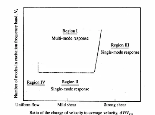
Vandiver at al. (1996) presented a categorization based on the shear factor in Equation(3.18), which suggested when single mode versus multi-mode responses might be expected. This categorization was based on model tests done in uniform and shear flow. Vandiver et al. observed that under highly sheared conditions some single-mode behavior was seen, Figure 16.

(34)

Figure 16 - Identification of multi-mode and single mode response regions. Vandiver et al. (1996) Higher Harmonics

Higher harmonic VIV response has been discussed in the offshore engineering literature for over twenty-five years. In-line vibration at twice the cross-flow vibration frequency is common knowledge and has been associated with figure-eight motions since the early 1980s [Vandiver 1983; Vandiver and Jong 1987]. The third and fifth harmonics were noticed in accelerometer measurements described in the late 1980s [Vandiver and Chung 1988], but were not considered to be of significant concern when making fatigue life estimates. This was because the response at the frequency of the third and fifth harmonics was quite small in these early experiments on flexible cylinders at low-mode number in uniform and sheared flows.

These experiments were primarily at low-mode number: second, third, or perhaps fourth mode. In the recent experiments, the twentieth to thirtieth modes were excited at the vortex shedding frequencies and large response was observed at higher harmonics of the vortex-shedding frequency.

In the early experiments, the low-mode number and low modal density did not favor the occurrence of resonance between the third harmonic of the lift force and a pipe

(35)

natural frequency. In the recent experiments, the third harmonic corresponds to approximately the 60th modal natural frequency. Adjacent natural frequencies are very close together and significant response is always possible. A frequency shift of less than 2% moves the mode number from fifty-ninth to the sixtieth.

Recently, Jauvtis and Williamson [2004] studied VIV for spring mounted cylinders having relatively low mass ratios (<6) and two degrees of freedom. They found the excitation at the 3x harmonic is associated with the shedding of three vortices in the wake behind the cylinder during each VIV half cycle. They call this the ‘2T’ mode of vortex shedding. They report that the switch to the 2T mode happens around reduced velocities of 5 and persists until reduced velocities of 8. They observed large Ay/Do ratios

associated with the 2T mode and call it the SuperUpper (SU) region in the plot of Ay/Do

versus reduced velocity. The 2T mode is associated with a relatively large third harmonic lift force component in the cross-flow direction.

Figure 17 shows Jauvtis’ and Williamson’s Ay/Do versus reduced velocity data.

This plot has been constructed from data shared by Williamson. The horizontal axis is Vr

reduced velocity based on the observed vibration frequency. The data is the same as that presented in Jauvtis and Williamson [2004], in which the data was plotted using a reduced velocity based on the still-water natural frequency. In order to compare the Jauvtis and Williamson data to the observations from the Gulf Stream and Lake Seneca experiments, the reduced velocity must be expressed in terms of observed response frequency, as in Figure 17. The region labeled as SU is the response branch associated with a strong 3x harmonic force component.

(36)

4 4.5 5 5.5 6 6.5 7 7.5 8 0 0.2 0.4 0.6 0.8 1 1.2 1.4 1.6 A Y /D o Reduced Velocity

Figure 17 - The SuperUpper (SU) region where the '2T' mode of vortex shedding is found [Jauvtis and Williamson 2004] using the Reduced Velocity (Vrn)

(37)

Chapter 4: Time Sharing of Dominant VIV Frequencies

Introduction

A long-discussed question in VIV is when does a single-frequency response happen and when does a multi-frequency response happen. The Lake Seneca tests were uniform-flow tests and single-frequency response was expected. The Lake Seneca tests can be used as a baseline for studying the difference in single- and multi-frequency responses.

The Gulf Stream tests provided a perfect opportunity to investigate the difference between single-frequency and multi-frequency behavior. After close examination of the data, it appears that single-frequency response happens all the time, but in sheared flows the single dominant frequency changes quickly in time. Using Maximum Entropy Method (MEM) analysis, [Burg 1968], the data could be analyzed on small time scales. When looking at short time segments, only one frequency dominated at any one time, but the frequency changed quickly in time.

Modal Behavior

A large number of tests have been done on cylinders at low mode number both in the laboratory and in the field. In these tests, single-frequency response is associated with a modal response. The RMS response shows clear nodes and anti-nodes. Figure 18 shows an example of this modal behavior for an instrumented riser. At these low-mode number cases, single-frequency behavior is controlled by a single mode.

At high mode number, the dynamics of the riser are different. The riser has more behavior of the infinite string than the finite length pinned-pinned string. Therefore, standing mode behavior is not seen at high-mode number. Instead, a single frequency response is seen. The modal behavior with nodes and anti-nodes is not seen at high mode numbers; instead, fairly uniform RMS response is seen in the power-in region with a damped decay outside the power-in region. Therefore, it is inaccurate to discuss singe-mode behavior at high-singe-mode number; instead, the system is dominated by a single frequency response.

(38)

Figure 18 – RMS Profiles of riser displacement and modal weight factors from an NDP drilling riser test [Kaasen et al 2000]

Resonant Behavior at High Mode Number

At low-mode number, resonant behavior is associated with modal behavior. When the frequency of vibration is close to a natural frequency of the cylinder, the vibrations are amplified or they “lock-in”. For high-mode numbers, resonant behavior is more associated with large amplitude response that is caused by coherent narrowband forcing lift forces. The resulting motion at the same frequency is sufficiently large to prevent vortex formation at competing frequencies. The vibrations interact with the wake formation so as to amplify, not dampen the response.

Current prediction programs, such as SHEAR7, allow multiple excitation frequencies to co-exist. This method allows different frequencies to have different non-overlapping power-in regions that abut one another. This new concept of single-frequency behavior, says that the frequencies share in time rather than space. This concept only holds true for resonant behavior, where resonant behavior is when large amplitude vibrations occur over an extended region of the pipe.

Local small amplitude vibrations can occur outside of a region with large amplitude response. These vibrations are localized to a small area, are caused by the local

(39)

current velocity, and are only slightly larger amplitude than the background noise. The vibrations are damped before they can travel to other areas of the pipe. Local small vibrations appear to be precluded from the areas that have a resonant behavior

Uniform Flow Cases

The Lake Seneca tests had uniform and uni-directional flow. Since the lake was still water, the flow was created by dragging the pipe through the water, [Vandiver et al, 2004]. This created known current speed and flow in only a single direction. The speed of the test was controlled by the speed of the boat that was towing the pipe. The speed control of the boat was not particularly precise, and the current speed varied somewhat over the course of the approximately 2.5 minute runs.

Figure 19 shows the Power Spectral Density (PSD) of a typical constant speed run at Lake Seneca. Because the towing speed was fairly constant and uniform, a single-frequency response is expected. The dominant VIV response is narrow-banded, with components that are harmonics of the dominant VIV frequency also contributing to the spectrum.

In Figure 20, a set of spectra is shown. Each spectrum is from 8.5 seconds of data. The spectra are in time sequential order, with the top spectrum being the first. There is no overlap in time between the spectra. The frequency is stationary, but amplitude varies, especially that of the third harmonic.

To look at the data on a longer time scale, a waterfall spectrum can be used. Burg MEM analysis was used to create Figure 21. Each increment contains 17 seconds of data, with 95% overlap. By looking at the dominant VIV frequency, one sees that only one frequency dominates at any one time. The change in frequency is likely caused by small variations in the current.

(40)

0 2 4 6 8 10 12 14 16 18 20 0 5 10 15 20 25 30 35 40 45 50 Frequency (Hz) P S D o f A c c e le ra ti o n

Figure 19 – Spectrum of 138 seconds of data from the Lake Seneca test.

0 2 4 6 8 10 12 14 16 18 20 0 10 20 30 0 2 4 6 8 10 12 14 16 18 20 0 10 20 30 P S D o f A c c e le ra ti o n 0 2 4 6 8 10 12 14 16 18 20 0 10 20 30 Frequency (Hz)

Figure 20 - A series of spectra in time increments of 8.5 seconds showing the dominant VIV frequency and the three-time harmonic component.

(41)

0 2 4 6 8 10 0 20 40 60 80 100 120 0407141419 Frequency (Hz) T im e ( s ) 20 40 60 80 100 120

Figure 21 – Waterfall spectra for a base case from Lake Seneca. Each time step used 4.2 seconds of data with 95% overlap

Sheared-Current Time Sharing

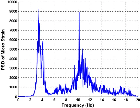
When a Power Spectral Density (PSD) is taken over one minute, up to 6 dominant frequencies may have happened in that time, and would all appear in the FFT. When the data is broken into very small time increments and analyzed, single-frequency response becomes more evident.

Figure 22 shows the spectra taken over two minutes for one strain gauge. The dominant VIV frequency shows multi-frequency participation. In Figure 23, the same time series is broken into 10-second intervals. The first two intervals show single-frequency resonant behavior. The second two intervals show the transition from one dominant frequency to another dominant frequency. The vibration at the original frequency loses energy as the second frequency builds up energy in vibration.

The existence of time-sharing does not prevent all multi-frequency behavior. Multi-frequency behavior happens at two different scenarios. The first scenario is seen in Figure 23, in the final two ten-second intervals. There is multi-frequency behavior as the vibrations change from one frequency to another. One frequency will be dominant, then another frequency will begin to gain energy, and the first frequency will lose energy.

(42)

0 2 4 6 8 10 12 14 16 18 20 0 1000 2000 3000 4000 5000 6000 7000 8000 9000 10000 Frequency (Hz) P S D o f M ic ro S tr a in

Figure 22 - Spectrum of 134 seconds of data from the Gulf Stream Bare Test

0 2 4 6 8 10 12 14 16 18 20 0 5000 10000 0 2 4 6 8 10 12 14 16 18 20 0 5000 10000 P S D o f M ic ro S tr a in 0 2 4 6 8 10 12 14 16 18 20 0 5000 10000 0 2 4 6 8 10 12 14 16 18 20 0 5000 10000 Frequency (Hz)

(43)

Multiple frequencies can exist at the same time in the Gulf Stream and Lake Seneca data. When this phenomenon occurs the amplitudes of the vibrations are small. When multi-frequency behavior is apparent, the amplitude of the spectral peak is less than 30% of the amplitude at resonant behavior.

The apparent behavior of the riser exhibits small locally generated vibrations that are damped before they travel more than one wavelength. When a resonance occurs, local vibrations are prevented by the coherent vortex shedding at the resonance frequency. The resonant-behavior vibrations are damped as they travel away from the region with a coherent wake. At sufficient distance from the excitation region, locally generated vibrations may be seen again.

Figure 24 is a waterfall spectrum of the same case. The dominant VIV frequency is seen to be about 4 Hz. When the amplitude of the vibration is at less than 1e4 εµ/Hz, some smeared behavior of multi-frequency participating is seen, but when the amplitude is large only one dominant frequency is apparent.

0 2 4 6 8 10 12 14 16 0 20 40 60 80 100 120 20041029171957 Frequency (Hz) T im e ( s ) 0.5 1 1.5 2 2.5 3 3.5 x 104

Figure 24 - Waterfall spectra of the strain gauge from the Gulf Stream Bare Case. Each spectrum was calculated using MEM analysis with a 5 second window and 80% overlap.

Figure 25 shows the same waterfall spectrum, but each time step has been normalized such that the maximum value is one. This shows that for most time steps that

(44)

no other dominant VIV frequency is greater than 50% of the magnitude of the dominant VIV frequency. 0 2 4 6 8 10 12 14 16 0 20 40 60 80 100 120 20041029171957 Frequency (Hz) T im e ( s ) 0.1 0.2 0.3 0.4 0.5 0.6 0.7 0.8 0.9

Figure 25 - Waterfall spectra of the strain gauge from the Gulf Stream Bare Case. Each time step is normalized to the largest peak. Each spectrum was calculated using MEM analysis with a 5 second window and 80% overlap.

Impact

The largest impact of time sharing is on the result of fatigue calculations. The calculations of the damage rate for a narrow-banded process, such as single frequency response are different from those for broad-banded or multi-frequency responses.

Common industry practice for the estimation of fatigue damage of risers is to use S-N curves. The fatigue curve for the riser is characterized by the equation NSb=C, where N being the number of cycles to failure, S is the RMS stress range, and b and C are parameters that best fit the data for a given material. When the time history of the stress is a constant stress range sinusoidal process, the damage rate, Dr, is given by:

( )

2 2 b n yr r T D S C ω π = (4.1)

(45)

If the stress history is a narrow-banded Gaussian random process, then the damage rate is, [Vandiver and Li 2003]:

(

)

2 2 2 2 b n yr r rms T _b D S C

ω

π

+   = _{Γ } _   (4.2)

Equation (4.1) is based on a sinusoidal distribution. Since VIV is rarely a constant amplitude sinusoidal function even with single frequency, Equation (4.2) is a better approximation of the damage. The damage caused by a single-frequency constant-amplitude sinusoidal input is the greatest damage. With single frequency time sharing, the damage rate is higher than it would be for a multi-frequency response, because the damage rate for a single frequency response is higher than the damage rate for a multi-frequency response. Unfortunately, there is no simple equation to describe the damage rate of a broadband spectrum. [Dirlick 1985].

Conclusions

The concept of time-sharing of dominant frequencies as opposed to multiple frequencies participating simultaneously is based on the data from the Gulf Stream and Lake Seneca tests. Single-frequency, time-shared response happens when significant zones of the riser are excited by spatially coherent single frequency forces. Multi-frequency response can happen with small amplitude locally generated waves. Time-sharing of single-frequency responses, as opposed to multi-frequency responses, has an effect on the damage rate of the riser.

(46)

Chapter 5: Finding the Power-In Region

Introduction

When looking at the current profile’s effect on a pipe, questions of which section of the pipe will allow power to enter the system, known as the power-in region, and which areas of the pipe act to damp the structure become important.

On short pipes at low-mode number, standing wave responses are seen. In the Lake Seneca and Gulf Stream experiments, the length-to-diameter ratio is greater than 3500. Additionally the pipes are responding at modes greater than 10th. At these mode numbers standing wave behavior over the entire pipe is not observed. Instead, a finite power-in region is observed with traveling waves leaving the power-in region and propagating to other regions.

Presented here are two methods of finding the power-in region, the reduced velocity method and the coherence mesh. The first method uses the local reduced velocity to determine whether points are in the power-in region. Reduced velocities from 5 to 8 are traditionally associated with large VIV response at sub-critical Reynolds number.

The second method uses a coherence calculation to find the range over which the vibrations are linearly dependant. The large amplitude waves that are generated in the power-in region will be coherent over a large range, whereas the local small vibrations will not be coherent over a large range.

Reduced Velocity Method

In the Lake Seneca and Gulf Stream experiments, reduced velocities from approximately 3 to 7 were observed by correlating the largest RMS strain response to the reduced velocity. Reduced velocities of 4.5 to 6.5 are observed in the regions with the largest RMS strain response.

Figure 26(a) shows the normal incidence current profile for a run from the Gulf Stream test with both speed (blue) and direction (green). The current profile is sheared from 1.5 ft/s to 3.0 ft/s. Figure 26(b) shows the total RMS strain (blue) and the RMS strain filtered to only contain the dominant VIV frequency (green).

(47)

(a) (b)

Figure 26 – Gulf Stream bare case (a) Current Speed (blue) and current direction (green); (b) RMS strain (blue) and RMS strain filtered to only show the contribution of the dominant VIV frequency.

Figure 27(a) shows the same current profiles as Figure 26. Figure 27(b) shows the dominant VIV frequencies for each location. The frequency that dominates for the most time is shown with the blue vertical line. The error bars show the variation of the dominant VIV frequency during the total record. In the power-in region, the variation in the frequency is seen to be similar and fairly constant.

Figure 27(c) shows the reduced velocity, calculated using the frequency of vibration. As the frequencies change with time sharing, the reduced velocities change at each location. The reduced velocities are also shown with error bars to show the shift in reduced velocity caused by the shift in frequency over the entire time history.

At the top of the pipe, the variation in reduced velocity is larger. The top of the pipe is an area with low RMS strain and is unlikely to be the power-in region. In this areas, traveling waves from the power-in region will sometimes dominate, which would cause the frequency to appear to be the same as in the power-in region. At other times,

-500 -450 -400 -350 -300 -250 -200 -150 -100 -50 0 1 2 3 4 5 D e p th a lo n g P ip e ( ft ) Current Speed (ft/s) -500 -450 -400 -350 -300 -250 -200 -150 -100 -50 00 45 90 Direction (degrees) 0 100 200 300 -500 -450 -400 -350 -300 -250 -200 -150 -100 -50 0 RMS Strain µµµµεεεε D e p th a lo n g P ip e ( ft ) 20061020182045 Current Direction Current Speed RMS Strain

(48)

locally generated small amplitude waves that are caused by local currents will dominate. This causes for much greater variation in the frequency, because the local current speed and the current speed in the power-in region can be significantly different from each other.

(a) (b) (c)

Figure 27 – Gulf Stream bare case (a) Current speed (blue) and the current direction (green); (b) Dominant VIV frequency, showing the most common frequency with the vertical line and the varying frequencies due to time sharing; (c) the reduced velocity, using dominant VIV frequency, the

variance is due to the variation in frequency with time shifting. Coherence Mesh

This method involves calculating the coherence from one sensor in a quadrant to every other sensor in the same quadrant. Coherence is a commonly used signal processing tool that shows linear dependence between to signals and is defined as:

( )

_{( ) ( )}

( )

2 xy xy xx yy P f C f P f P f = (5.1) -500 -450 -400 -350 -300 -250 -200 -150 -100 -50 0 1 2 3 4 D e p th a lo n g P ip e ( ft ) Current Speed (ft/s) -500 -450 -400 -350 -300 -250 -200 -150 -100 -50 00 45 90 Direction (degrees) -500 -450 -400 -350 -300 -250 -200 -150 -100 -50 0 2 4 6 Frequency (Hz) 20061020182045 -500 -450 -400 -350 -300 -250 -200 -150 -100 -50 0 4 6 8 Reduced Velocity Current Direction Current Speed