HAL Id: hal-00414760
https://hal.archives-ouvertes.fr/hal-00414760
Submitted on 16 Nov 2019
HAL is a multi-disciplinary open access
archive for the deposit and dissemination of
sci-entific research documents, whether they are
pub-lished or not. The documents may come from
teaching and research institutions in France or
abroad, or from public or private research centers.
L’archive ouverte pluridisciplinaire HAL, est
destinée au dépôt et à la diffusion de documents
scientifiques de niveau recherche, publiés ou non,
émanant des établissements d’enseignement et de
recherche français ou étrangers, des laboratoires
publics ou privés.
Ionization processes in the atmosphere of Titan. II.
Electron precipitation along magnetic field lines
Guillaume Gronoff, Jean Lilensten, Ronan Modolo
To cite this version:
Guillaume Gronoff, Jean Lilensten, Ronan Modolo. Ionization processes in the atmosphere of
Ti-tan. II. Electron precipitation along magnetic field lines. Astronomy and Astrophysics - A&A, EDP
Sciences, 2009, 506, pp.965-970. �10.1051/0004-6361/200912125�. �hal-00414760�
Received 20 March 2009/ Accepted 13 July 2009
ABSTRACT
Context.The Cassini probe regularly passes the vicinity of Titan, providing new insights into particle precipitation by use of its electron and ion spectrometers. A discrepancy between precipitation models and observations of electron fluxes has been found. This discrepancy was suspected to be caused by the geometry of the magnetic field.
Aims.In this article, we compute the electron impact ionization in the nightside ionosphere of Titan, assuming non-trivial geometry for the magnetic field lines.
Methods.We use the TransTitan model, modified to take into account the magnetic field line geometry in the nightside, and we com-pare these results with the electron flux measurements during the T5 fly-by of Cassini. We use several magnetic field line geometries, including one produced by hybrid simulations.
Results.The geometry of the lines implies a longer path of the electron inside the atmosphere of Titan. The electron fluxes are therefore modified considerably compared to the vertical precipitation hypothesis. At an altitude of 1200 km, the electron flux can be divided up to ten times with a field line resulting from hybrid simulation. Thanks to the use of more accurate field lines, the model reproduces the experiment well without any further adjustment of the precipitated measured electron flux.
Conclusions.Several hypothesis had been suggested to explain the discrepancies between the different models and the observation of the electron flux during the T5 fly-by of Cassini. Our approach shows that the most probable explanation is the magnetic field line geometry. This work shows that the computation of ion production by electron impact in the atmosphere of Titan needs the consider-ation of both magnetic field and the input electron fluxes. Based on these considerconsider-ations, our model can compute the conditions for future fly-by, and could be used to compare models with experiments.
Key words.planets and satellites: individual: Titan – atmospheric effects – space vehicles: instruments
1. Introduction
The magnetic environment of Titan in the magnetosphere of Saturn is very complex, and its characterization and compre-hension is one of the main objectives of the Cassini’s probe mission (Blanc et al. 2005). Because of the absence of an in-trinsic magnetic field, Titan’s atmosphere and ionosphere inter-act directly with Saturn’s magnetospheric plasma (Backes et al. 2005). The upper atmosphere is thus partly ionized by mainly solar photons and electron impact. The strength and location of each ionization source is sensitive to the orbital location of Titan, leading to a very complex ionized environment and being highly dynamic. Cassini observations have suggested that photoionisa-tion is the most important ionizaphotoionisa-tion process for Titan’s dayside (Agren 2009, submitted to PSS). On the other hand, Cassini observations have also shown that, on the nightside, electron impact plays an important role and is the main source of ion-ization (when the nightside corresponds to the ram-side). This situation happened on April 16th, 2005 on the outbound pass of the T5 flyby by the Cassini spacecraft. The electron flux data acquired during this flyby was compared with several models (Agren et al. 2007; Cravens et al. 2008). These comparisons showed that the ionization and the fluxes detected by the Cassini probe cannot be modeled as a vertical precipitation. This can be interpreted as a consequence of the interaction between the
mag-netic field lines and the atmosphere of Titan (Cravens et al. 2009; see also, Gronoff et al. 2009, Paper I – Ionization in the whole at-mosphere, this issue). In this paper, we use the TransTitan model to compute the electrons fluxes at different altitude by consider-ing different geometry of magnetic lines.
2. The TransTitan model
To compute the electron fluxes in different geometric configura-tions, we need a code capable of computing electron transport in the atmosphere. In particular, it must compute the influence of elastic and inelastic collisions with the different species of the atmosphere. This code exists: TransTitan, which has been stud-ied in details in the Paper I. In the present paper, we only use the kinetic part for the electrons in the nightside. The geometry of the code is modified to take into account the bending of the mag-netic field lines around Titan: in the original version of the code, the electron transport was computed along a straight line, which cannot be strongly inclined with respect to the vertical. The verti-cal line represents the grid where the ionization is computed. In the present version, we compute the ionization along the mag-netic field line. For this study, the neutral atmosphere used is described inCui et al. (2009), and we take into account only the densities of the two major components of the atmosphere, N2and CH4. To study the influence of the neutral atmosphere,
966 G. Gronoff et al.: Ionization processes in the atmosphere of Titan. II.
Fig. 1.The different neutral atmosphere considered. For the main
sim-ulation, theCui et al.(2009) neutral atmosphere, coming from Cassini observations, is used. It has a lower density in CH4 and N2 than the
Waite et al.(2005) neutral atmosphere (Cassini observations). The pre-Cassini model ofMüller-Wodarg et al.(2000) (labeled M-W in the fig-ure) is mainly at a higher density for the two species, the CH4mixing
ration was supposed to be more important than the recent observations.
we also used the neutral atmosphere ofWaite et al.(2005) and the pre-Cassini model ofMüller-Wodarg et al.(2000). The dif-ferences between these models can be seen in Fig.1. The main difference is that the pre-Cassini model has a higher CH4density
in the upper atmosphere. We assume that the exospheric temper-ature is constant at 175 K. The altitude range covered by our computation is from 900 km to 1600 km, the lower altitude be-ing determined by the geometry of the line. The correspondbe-ing length of the lines can be more than 4000 km.
3. Electron precipitation and magnetic field line geometry
In situ electron-flux spectra are taken fromCravens et al.(2009). The aim of this present work is to compute the ionospheric pa-rameters, by taking into account the presence of the Kronian magnetic field and mimicking the behavior of the electron fluxes, which are affected by the magnetic field draping. So far, vertical magnetic field lines or parabolic lines have been used to compute the electron energy deposition in Titan’s atmosphere (Cravens et al. 2005). We assume several magnetic field line configura-tions, including horizontal magnetic field lines above 1200 km. Titan’s ionosphere acts as an obstacle and modifies the magne-tospheric plasma flow. The kronian magnetic field lines close to Titan are twisted and wrap the ram-side of the body, as they dif-fuse slowly in the dense and cold ionosphere. We assume curved magnetic field lines, which enter inside the ionosphere to emerge outside several thousand of kilometer apart. To demonstrate how the magnetospheric electron fluxes are sensitive to the magnetic field line topology, we use simulation results describing the drap-ing around Titan. These field lines are extracted from a three-dimensional multi-species hybrid simulation. In this model, a kinetic description is used to describe ions, while electrons are characterized as an inertialess fluid contributing to electric cur-rents that produce quasineutrality. This model depicts the dy-namics of the plasma environment in the vicinity of Titan, and includes the effects of ionization by solar photons, ionization by
Fig. 2.Electron precipitation flux in the atmosphere of Titan as mea-sured by Cassini ELS instrument, at an altitude of 2730 km (Cravens et al. 2009). The dots represents the measurement, the line represents the values used in our model. An interpolation has been made be-tween 0.3 and 1 eV.
electron impact, and charge exchange. We note that the descrip-tion below 1400 km is limited in this model since the complex ionospheric chemistry is not included. Nevertheless, the model describes the photoabsorption and the deceleration of ions in the atmosphere caused by elastic collisions. More details concern-ing the model are presented inModolo & Chanteur(2008). The different configurations are summarized in Fig. 3, where each number corresponds to the following cases:
1. the vertical case;
2. a straight line with a minimum altitude at 1200 km; 3. a straight line with a minimum altitude at 1000 km; 4. a bent line with a minimum altitude at 1200 km; 5. a bent line with a minimum altitude at 1000 km;
6. the hybrid simulated line. This line is cut at the lowest alti-tude of 1000 km because the simulation is not valid below. To show the draping at the origin of this line, we put two other simulated lines (label 7), which does not reach the alti-tude of our simulation.
4. Result
Given the incident precipitation flux shown in Fig.2, we consid-ered the impact of several magnetic geometries on the produc-tion and fluxes at different altitudes.
4.1. First case: vertical precipitation
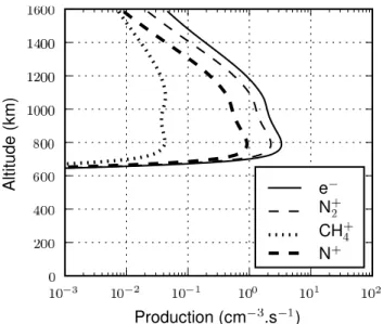
This is the simplest case, we consider that electrons simply precipitate vertically. The resulting ionization can be seen in Fig. 4. The ionization peak is at 800 km, and has an inten-sity of 3 cm−3s−1, this simulation having been completed us-ing theMüller-Wodarg et al.(2000) neutral atmosphere, because electrons reaches the mesosphere. We computed the resulting electron flux (which corresponds to the degradation in energy
Fig. 3.Magnetic field line geometry used in the simulations. The two straight lines have a minimum altitude of 1200 and 1000 km respec-tively, as is also true for the two bent lines. The long line corresponds to hybrid simulations. The angle corresponds to a curvilinear projection: the length on the picture corresponds to the line length, this projection being useful when solar source is not taken into account, as in this paper. The arrows show where the electrons are precipitating in our model, and the large black numbers indicate the simulation number (see the di ffer-ent cases) corresponding to each line. The number 7 shows additional lines from the hybrid simulation, above the altitude of the present study.
Fig. 4.Electron impact ionization in the (first) case of a vertical mag-netic field line. CH+4 is produced by electron impact ionization on CH4.
N+2 and N+are produced by electron impact ionization on N2. In this
fig-ure, theMüller-Wodarg et al.(2000) neutral atmosphere has been used because electrons reach the mesosphere, which is not described in the other neutral models.
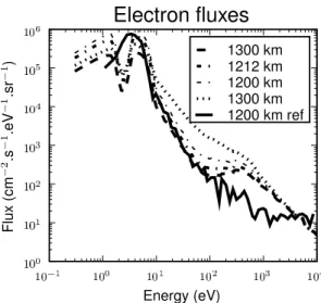
of the primary flux plus the secondary electron flux) at differ-ent altitudes (Fig. 5, with the Cui et al. 2009, atmosphere in that case). We find a significant discrepancy between the Cassini flux measured at 1200 km and the model predictions. As in
Fig. 5.Comparison of the modeled fluxes in the (first) vertical case at several altitude with 1200 km altitude Cassini measurements. This sim-ulation shows that we cannot compare the vertical precipitation hypoth-esis with data. To compare with the result of the flux division hypothhypoth-esis (Cravens et al. 2009), we added the results of that hypothesis, labeled “1200 km, ref”.
Agren et al.(2007) andCravens et al.(2009), we have to divide the input flux by a factor of about 10 to reach good agreement. As shown in Fig.5, that hypothesis allows us to explain the flux in the 10–1000 eV energy range, but underestimates the flux at both lower and higher energies.
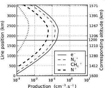
4.2. Second case: straight line, horizontal at 1200 km In that case, we use a straight horizontal line, whose lower al-titude is 1200 km, e.g., it is perpendicular to the vertical at this altitude. This geometry could not be simulated with the initial TransTitan code. The maximum altitude of this line is the top of our atmosphere at 1600 km, and corresponds to the line with a 3500 km entry in the thermosphere and 0 km exit of the ther-mosphere, in Fig. 6. In that figure, we can see that the ion-ization peak is not at the middle of the line, but at 2300 km, with an intensity of 0.3 cm−3 s−1. The corresponding altitude
is 1230 km, but is about 500 km away from the lowest point (1200 km altitude). The corresponding flux comparison can be seen in Fig.7, the agreement being closer than in the previous case: the 1789 km length flux is inside the measurement error bars between 10 eV and 200 eV, and corresponds to an altitude of 1200 km. This results shows that the division of the input flux is unnecessary to account for this part of the spectrum. For the highest energy, our modeling departs from the measurements, being one order of magnitude higher in flux.
4.3. Third case: straight line, horizontal at 1000 km
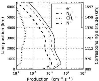
This case is similar to the previous one, except that the lower altitude of the line is 1000 km and the maximum altitude is al-ways 1600 km, which is reached at the extremities. The ion pro-duction maximum occurs at 3000 km length, with an intensity of 0.5 cm−3 s−1 (Fig. 8). The peak corresponds to an altitude
of 1100 km. The corresponding flux comparison can be seen in Fig.9, where, fluxes at altitudes close to 1000 km show agree-ment with measureagree-ments when energies are above 500 eV.
968 G. Gronoff et al.: Ionization processes in the atmosphere of Titan. II.
Fig. 6.Electron impact ionization in the (second) horizontal 1200 km case.
Fig. 7.Comparison of the fluxes at several altitude in the second case (horizontal, 1200 km) with 1200 km altitude Cassini measurements. The altitude of 1245 km corresponds to an abscissa of 1192 km. The 1200 km one to 1789 km, the 1247 one to 2385 km, and the 1292 one to 2624 km. The higher the curvilinear abscissa is, the closer it is to the precipitation source.
4.4. Fourth case: bent line, minimum at 1200 km
In this simulation, we use a curved line with a minimum alti-tude at 1200 km (Fig.3). The ionization peak is at 1200 km length, which corresponds to an altitude of 1210 km. Its inten-sity is 0.3 cm−3 s−1(Fig.12). The corresponding flux
compari-son can be seen in Fig.11. A more accurate description of the reference flux is achieved for an altitude of 1300 km, where the magnetic field line goes outside of the atmosphere.
4.5. Fifth case: bent line, minimum at 1000 km
This is the same configuration as in the previous case, except that the lower altitude is 1000 km. The ionization peak is at 1700 km length, which corresponds to an altitude of 1100 km. Its intensity is 0.9 cm−3s−1(Fig.12). The corresponding flux comparison can
be seen in Fig.13. The fluxes simulated below 1100 km are very close to the reference flux. For the two bent cases, we can con-clude that it is possible to find a magnetic field line configuration
Fig. 8.Electron impact ionization in the (third) horizontal 1000 km case.
Fig. 9.Comparison of the fluxes at several altitudes in the third case (horizontal, 1000 km with 1200 km altitude Cassini measurements). The altitude of 1200 km corresponds to an abscissa of 3390 km. The 1090 km one to 2957 km, the 1060 one to 2813 km, and the 1018 one to 2524 km. The higher the curvilinear abscissa is, the closer it is to the precipitation source.
capable of explaining the entire spectrum without modifying the input energy spectrum. However, to determine the reality of this approach, we need to use global simulation computed lines. 4.6. Sixth case: line from a hybrid simulation of the Ta fly-by
of Cassini
In this case, we use a magnetic field line computed from a hy-brid simulation performed in the conditions of the Ta fly-by of Cassini (Modolo & Chanteur 2008).
We considered several magnetic field lines in that simulation, and we only show the one that provide closer agreement with measurements. This line is of course an approximation, used as a representative field line when Titan is inside the magnetosphere of Saturn: the measurement were completed for the T5 fly-by and the MHD simulation is incomplete below 1400 km. The ion-ization peak is at 500 km length, which corresponds to an alti-tude of 900 km. Its intensity is 0.5 cm−3s−1(Fig.14). The
Fig. 10. Electron impact ionization in the (fourth) bent 1200 km case.
Fig. 11.Comparison of the fluxes at several curvilinear abscissa in the fourth case (bent, 1200 km) with 1200 km altitude Cassini measure-ments. The altitude of 1300 km corresponds to an abscissa of 566 km. The 1212 km one to 884 km, the 1200 one to 1111 km, and the 1300 one (dots) to 1557 km. The higher the curvilinear abscissa is, the closer it is to the precipitation source.
between model and experiment is good and within the error bars in that case, even if a difference is still seen in high energies.
5. Discussion
Cravens et al.(2009) consider the problem of the discrepancy be-tween the vertical precipitation model and the comparison of the fluxes at 1200 km. In Fig.5, we confirm this problem, with the important discrepancy between our model and the experiment at this altitude. The conclusion of this work was that the elec-trons are embedded in different magnetic tubes, each one having a different electron flux.
In the present work, the use of several magnetic field con-figurations shows that the geometry of the precipitation has an important effect on the electron flux at 1200 km altitude. In Figs.7and15, we find good agreement between model and ex-periment, between approximatively 10 eV and few hundred eV. The differences at high energies could be explained by the spa-tial resolution: in Fig.15, the high energy fluxes vary signifi-cantly between 1200 km altitude and 1130 km altitude. Another
Fig. 12. Electron impact ionization in the (fifth) bent 1000 km case.
Fig. 13.Comparison of the fluxes at several curvilinear abscissa in the fifth case (bent, 1000 km) with 1200 km altitude Cassini measurements. The altitude of 1000 km corresponds to an abscissa of 1253 km. The 1020 km one to 1462 km, the 1200 one to 1921 km, and the 1300 one to 2088 km. The higher the curvilinear abscissa is, the closer it is to the precipitation source.
explanation of this discrepancy could be that in the neutral at-mosphere model used in our simulations, or in the uncertainties in the flux measurement at these energies. Concerning the influ-ence of the neutral atmosphere, some minor differences in the fluxes are visible when we replace theCui et al.(2009) model with either theWaite et al.(2005) or theMüller-Wodarg et al. (2000) model. However, the neutral atmosphere cannot notably explain the differences between model and experiment in the ver-tical case. In Fig.16, we can see the resulting flux at 1200 km for the hybrid simulated line with the different neutral atmo-spheres. The neutral atmosphere ofCui et al.(2009) produces higher fluxes (about two times higher between 10 and 1000 eV). This is because of the lower density of that model, although the model predictions are within the error bars of the observations. Further improvements will require either a precise measurement of the neutral atmosphere during the fly-bys or a neutral atmo-sphere model that considers the variation in the density with e.g., solar zenith angle, solar activity.
To identify which of the two possible explanations of the observed electron flux is the most appropriate at 1200 km, we
970 G. Gronoff et al.: Ionization processes in the atmosphere of Titan. II.
Fig. 14. Electron impact ionization in the Ta 1000 km case.
Fig. 15.Comparison of the fluxes at several curvilinear abscissa in the sixth case (Ta Fly-by) with 1200 km altitude Cassini measurements.The altitude of 985 km corresponds to an abscissa of 1087 km. The 1130 km one to 2174 km, the 1200 one to 2935 km, and the 1240 one to 3262 km. The higher the curvilinear abscissa is, the closer it is to the precipitation source.
need to measure the magnetic field line for the T5 conditions. Such work has not yet been published. The detection of a mag-netic field oriented to the vertical at 45◦along the Cassini’s path (Cravens et al. 2009) would be insufficient to retrieve the data by modeling, but would be able to constrain models. The obser-vation of the magnetic draping (Bertucci et al. 2008) shows that an analysis of the magnetic environment of Titan is necessary to compute the ion production caused by electron impact. The ion production in the different cases (Figs.7,9,11,13, and15) shows an enhancement in the production at high altitude, and a lack of production at low altitude.
6. Conclusion
The new version of TransTitan is able to compute electron pre-cipitation along magnetic field lines in the atmosphere of Titan.
Fig. 16.Influence of the models of neutral atmosphere on the computed flux for the simulated line. All fluxes are computed at an altitude of 1200 km to be compared with the reference flux. The neutral atmo-sphere is not the main explanation of the difference at high energy, but needs to be considered for precise comparison of model and data (The
Müller-Wodarg et al. 2000, atmosphere is labeled M-W).
Because of the magnetic field line geometry computed by hybrid simulation, we find agreement between model and observations of electron fluxes inside the atmosphere of Titan, without need-ing to divide the input flux. The magnetic field line geometry can therefore provide an explanation of the discrepancy between model and observation observed in Cravens et al. (2009), but lack of knowledge about the magnetic configuration still pre-vents us from being able to decide between our explanation and the hypothesis of magnetic tubes with different electron fluxes. The present work can be considered as a basis for future work on the comparison between MHD models and precipitation ob-servations on Titan and other non-magnetic planets or bodies. It illustrates the importance of considering draped magnetic field lines inside the atmosphere.
Acknowledgements. The authors wish to thank C. Simon (BIRA, Belgium), M. Barthélemy (LPG, France) and V. Vuitton (LPG, France) for useful discussions.
References
Agren, K., Wahlund, J. E., Modolo, R., et al. 2007, Annales Geophysicae, 25, 2359
Backes, H., Neubauer, F. M., Dougherty, M. K., et al. 2005, Science, 308, 992 Bertucci, C., Achilleos, N., Dougherty, M. K., et al. 2008, Science, 321, 1475 Blanc, M., Kallenbach, R., & Erkaev, N. V. 2005, Space Sci. Rev., 116, 227 Cravens, T. E., Robertson, I. P., Clark, J., et al. 2005, Geophys. Res. Lett., 32 Cravens, T. E., Robertson, I. P., Ledvina, S. A., et al. 2008, Geophys. Res. Lett.,
35
Cravens, T. E., Robertson, I. P., Waite, J. H., et al. 2009, Icarus, 199, 174 Cui, J., Yelle, R. V., Vuitton, V., et al. 2009, Icarus, 200, 581
G. Gronoff, J. Lilensten, L. Desorgher, & E. Flückiger, A&A, 506, 955 (Paper I) Modolo, R., & Chanteur, G. M. 2008, J. Geophys. Res., 113
Müller-Wodarg, I. C. F., Yelle, R. V., Mendillo, M., Young, L. A., & Aylward, A. D. 2000, J. Geophys. Res., 105, 20833