The dynamics of global financial crises

The Dynamics of Global Financial Crises

by

Rishi Kumar

Submitted

to the Department of Electrical Engineering and Computer Science

in partial fulfillment of the requirements for the degree of

Master of Engineering

in Electrical Engineering and Computer Science

at the

MASSACHUSETTS INSTITUTE OF TECHNOLOGY

June 2003

@

Massachusetts Institute of Technology 2003.

All rights reserved.

Author .

Department of Electrical Engineering and Computer Science

June, 2003

C ertified by ...

Andrew Lo

Harris & Harris Group Professor

Thesis Supervisor

Accepted by ...

Arthur C. Smith

Chairman, Department Committee on Graduate Students

MASSACHUSETTS INSTITUTE OF TECHNOLOGY

The Dynamics of Global Financial Crises

by

Rishi Kumar

Submitted to the Department of Electrical Engineering and Computer Science on June, 2003, in partial fulfillment of the

requirements for the degree of Master of Engineering

in Electrical Engineering and Computer Science

Abstract

This research aims to develop a Markov chain model of the transmission of financial crises. It uses a mathematical programming framework to determine the transition probabilities that describe the crisis dynamics. The framework allows for modelling and comparing various channels of contagion, such as investments and bilateral trade. Thesis Supervisor: Andrew Lo

Acknowledgments

I thank Professor Andrew Lo for advising this thesis. This work was made possible by the efforts of the Global Financial Crises team at the MIT Laboratory for Financial Engineering including Mila Getmansky, Kevin Amolirdviman and Eric Chemi.

Contents

3.2 Markov Chain Analysis . . . . 18

3.2.1 Markov Chains . . . . 18

3.2.2 States in Crisis Modeling . . . . 19

3.3 Mapping Global Relationships . . . . 20

3.4 Generating Transition Probabilities . . . . 22

3.5 A nalysis . . . . 25

3.5.1 Feasibility: Initial Feasible Solution . . . . 25

3.5.2 Optimality: Sanity Check . . . . 26

3.5.3 Tractability: Algorithmic Complexity, Runtime . . . . 27

4 Model Instantiation

4.0.1

Relationship Matrix: Bilateral Trade . . . .

4.0.2

Unconditional Crisis Probabilities . . . .

29 29 29 33 33 34 34 35 37 5 Results 5.1 Data . . . .

5.1.1

Trade Data

5.1.2

EMP Data.

5.2 Sample Results

.

.

5.3 Conclusion. . . . .

List of Figures

3-1 Contagion from Country A to Country C through Country B . . . . . 18

3-2 Contagion as a result of combined influence of two countries . . . . . 18

3-3 Markov States for Two Country Case . . . . 19

3-4 Two Country Markov Chain . . . . 20

3-5 _{Global Relationship Graph for 9 countries: Canada, USA, Brazil, Italy,} China, Fance, Mexico, United Kingdom, Germany . . . . 21

List of Tables

5.1 Sample Data for CaseI

.. .. . . . .

36

5.2 Sample Trade Data for Case1 . . . .

36

5.3 Sample Data for Case2 . . .. . . . .. . . . .. .

37

5.4 Sample Trade Data for Case2. . . . .. . . . .. . . . .

37

5.5 Sample Data for Case3 . . .. . . . .. . . . .

39

5.6 Sample Trade Data for Case3. . . . .. . . . .

39

5.7 Sample Data for Case4 . . .. . . . .

39

5.8 Sample Trade Data for Case4. . . . .. . . . .

40

5.9 Sample Data for Case5 . . .. . . . .

40

5.10 Sample Trade Data for Case5. . . . .

40

5.11 Sample Data for Case6 .. .. . . . .

41

5.12 Sample Trade Data for Case6 . . . .. . .

41

5.13 A sian Crisis . . . . 41

5.14 R ussia Crisis . . . . 41

5.15 Turkey Crisis . . . .. .. . . . . 42

Chapter 1

Introduction

Over the past decade, several financial and economic crises hit a number of developing countries. While some of these crises appeared to be isolated incidents affecting one country, for example, in Turkey and Argentina, a far greater number of them had effects beyond the borders of the initial country. In particular, the European Monetary System crisis of 1992, the Mexican crisis of 1994, the East Asian crisis of 1997, and the Russian crisis of 1998 affected more than the initial country.

The volatile nature of these crises resulted in economic hardship, political in-stability, and the toppling of a few governments. What made the crises even more disturbing was how they spread from country to country in an unexplained manner. The real difficulties associated with these financial crises prompted calls for the im-plementation of a variety of remedies from capital controls and currency boards to restrictions in the flow of foreign direct investment.

1.1

Problem Statement

This thesis develops a discrete-time stochastic model of the spread of a financial crisis from one country to another. The model for such contagion of financial crises is used to explore the paths a crisis can take through different countries. The thesis aims to make contributions in the following areas:

Markov chains in which each Markov state is a state of the world with some countries in a tranquil financial condition and some in crisis.

Mathematical Programming: To outline an optimization model in a mathemat-ical programming paradigm. This can be used to generate a set of transition probabilities between the Markov states that are in line with empirical data on

crisis probabilities and beliefs about contagion mechanisms.

Contagion Channels: The model developed allows for comparison of various chan-nels of contagion. For instance, crisis probabilities can be computed using bi-lateral trade data, credit or investment data. The results obtained can then be compared to assess the relative efficacy of the two channels in explaining contagion.

1.2

Thesis Overview

The next chapter, chapter 2, reviews the existing literature on the notion of contagion and approaches to modeling crises. Chapter 3 gives an overview of the Markov chain framework and the optimization program. Chapter ?? describes one instance of the model. Chapter 5 shows the application of the model to historical data.

Chapter 2

Literature Review

2.1

Types of Contagion

There are several related but distinct types of contagion. The most often analyzed type, financial contagion refers to the spread of financial crises from one country to one or more other countries. Typically, the spread of crises is marked by a sharp deterioration of several macroeconomic and financial variables such as a fall in an index of the stock market, a depreciation of the currency, decreased or negative GDP growth rates, net outflows of foreign investment, and the collapse of property prices. Although recent crises such as the East Asian crisis of 1997 have been accompanied by all of these effects, some of the recent literature has chosen to focus on currency crises as the signal that a financial crisis has occurred.

It is possible to imagine the contagion of other types of crises as well. One country may default on its sovereign debt, causing defaults in other countries (default conta-gion). The stock market in an emerging market might drop significantly followed by similar drops in other markets independent of a currency crisis (stock market conta-gion). Political upheavals may destabilize regions promoting turmoil in neighboring countries (political contagion). A few papers have looked at contagion using these other indicators of crisis (see, for example, Baig and Goldfajn, 1999).

There is no consensus on what makes up contagion. Forbes and Rigobon (2001) review some of the definitions of what constitutes contagion. Early papers often point

to some empirical phenomenon (for example, increased co-movement in short term interest rates, see Gerlach and Smets 1995) and try to explain it without explicitly defining contagion. The implicit assumption is that contagion has occurred and the papers tackle the question of defining its causes.

Testing for contagion of crises requires a definition of crisis. Several papers (see for example, Glick and Rose, 1999) use popular press accounts to determine the approximate start of a crisis. These types of tests have the appeal of attempting to explain the spread of an intuitive (or popular press) notion of crisis. Eichengreen, Rose, and Wyplosz (1996) point out that focusing only on instances of devaluation of the exchange rate could miss other significant episodes of market pressure. A crisis is often preceded by a speculative attack which hastens the devaluation of the currency. However, the monetary authorities could repel a speculative attack by raising interest rates. Additionally, the authorities could increase monetary reserves in non-crisis periods to preempt an attack. To account for these additional periods, Eichengreen, Rose, and Wyplosz devised an index of exchange market pressure (EMP) that incorporates the key tools that a monetary authority has at its disposal. Using the EMP index as a proxy for the incidence of a crisis, they estimate a binary probit model to test for the significance of various macroeconomic variables in explaining contagion.

2.2

Measuring Contagion

Rigobon (2001) explores a number of pitfalls in commonly used tests for contagion. Tests for contagion must account for simultaneous equations, omitted variables, and heteroskedasticity in the data. He specifically looks at the more widely adopted tests of contagion including linear regressions, logit-probit regressions, and tests based on Principal Components. He develops procedures to correct for these problems under special conditions. Forbes and Rigobon (2001) review the four different approaches that have been used to test for contagion: analysis of correlation coefficients, GARCH frameworks, cointegration, and probit models.

2.3

Mechanisms of Transmission

The literature on contagion has divided explanations for the transmission of financial crises into two types: fundamental links among economies and the behavior of in-vestors (Dornbusch, Park, and Claessens 2001). The fundamental links often cited as conduits of crises are trade and capital flows. Others point to rational and irrational investor behavior as another mechanism of crisis transmission.

2.3.1

Fundamental Mechanisms

Forbes (2001) reviewed the recent literature on the role of trade in transmitting crises. Gerlach and Smets (1995) present empirical evidence on the co-movement of interest rate spreads in Nordic countries during the 1992 EMS crisis. From this, they go on to develop a three-country model based on the Flood-Garber speculative attack model. They derive the time path of the exchange rates and show the dependence of the exchange rate collapse of one country on the collapse of another country. They build a story of how the collapse of the exchange rate in country 1 leads to a real appreciation of the exchange rate of country 2. This leads to a decrease in money demand in country 2 and an erosion of reserves. A decreased ability to defend the exchange rate in country 2 eventually leads to collapse. They predict that contagion effects would be stronger when wage flexibility is low and the degree of trade integration is high between the two countries relative to the anchor country.

In addition, a number of papers empirically estimate the importance of trade in transmitting crises. Glick and Rose (1999) attempt to distinguish the importance of trade and macroeconomic mechanisms in the transmission of crises. They regress the incidence of crises on an index of trade integration involving bilateral trade data. They find that trade better explains the spread of crises than macroeconomic similarity. Forbes (2001) uses bilateral trade data broken down by industry and attempts to separate the macroeconomic effects of changes of different types of trades. She divides the implications of changes in trade into three types: a competitiveness effect, where a depreciation in another country's exchange rate decreases the first country's ability

to export similar goods; an income effect, where a depreciation will sharply reduce exports to that country; and a cheap import effect, where the input prices will be reduced.

2.3.2

Investor Behavior

In 1998, a crisis in Russia led to a series of financial crises in a number of emerging markets seemingly unrelated by trade or other fundamentals to Russia. To explain this, Calvo (1999) develops a model where uninformed investors observe the actions of informed investors. The uninformed investors face a signal extraction problem where they are not sure whether the sales of assets by informed investors reflects negative information or margin calls. The actions of these uninformed investors tend to amplify movements in the price of emerging market securities even where the markets may not be linked by trade. In general, the co-movement of financial indicators in emerging economies may be explained by their dependence on a common set of investors.

The remaining chapters of this thesis present a model of global financial crises that illustrates the time path of contagion and allows for the analysis of contagion dynamics.

Chapter 3

Model

This chapter outlines the framework employed in modeling contagion. It presents the Markov chain formulation of the problem, the mathematical program for probability generation, and the mechanism for mapping global relationships.

3.1

Toward a Model of Dynamics

Much of the recent work has focused on presenting and testing the significance of various linkages between economies (for example, regional similarities, trade, and common investors). Less emphasis has been placed on explicit modeling of the dy-namics of the spread of a crisis. The course of a global crisis has large ramifications for investors, multinational corporations, and the people of the afflicted countries. When a neighboring country experiences a severe and unexpected financial crisis, it matters a lot whether your country will be next.

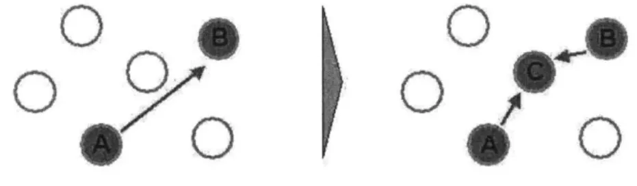
In the absence of a framework to model the dynamics of crises, several key fea-tures of the behavior of crises are overlooked. For instance, the health of a country may depend on the health of neighboring countries or on trade partners in complex ways which are not effectively captured in pairwise estimates. Figure 3-1 illustrates, through a two period example, how a crisis may spread from Country A to Country C through an intermediate Country B that is related to both A and B.

Coun-S

0

g

*0o

(

0

g*0

Figure 3-1: Contagion from Country A to Country C through Country B

try A to Country B. Neither a crisis in Country A nor the crisis in Country B are individually sufficient to cause a crisis are sufficient to cause a crisis in Country C but in the second period they together produce a combined effect that is sufficient to produce a crisis in Country C.

(

0

*

0Akh

0

S

/

*0

Figure 3-2: Contagion as a result of combined influence of two countries

Such effects are not sufficiently accounted for in the current schemes that attemp to model contagion. The comprehensive understanding of contagion of crises calls for the exploration of a dynamic model of crises dynamics and a broader model of inter-country dependencies.

3.2

Markov Chain Analysis

3.2.1

Markov Chains

Markov Chains are used to model stochastic processes. The dynamics of a financial crisis can be modeled using a Markov chain in which the Markov state changes at specific discrete time steps. At any time t, the current state is denoted by Xt. S

(

(

is the set of possible states.1 The Markov chain is described by a set of transition probabilities pij that denote the probability that the next state is equal to j given that the current state is i. Explicitly,

pi

= P(Xt+

=

jIXt

= i)

(3.1)

The key assumption underlying a Markov chain is that the transition probabilities pij apply whenever state i is visited with no dependence on the history of states visited in the past.

A Markov chain model specifies: (a) the set of states S = 1, ..., n, (b) the numerical

values of the transition probabilities from any one state to any other, pij.

3.2.2

States in Crisis Modeling

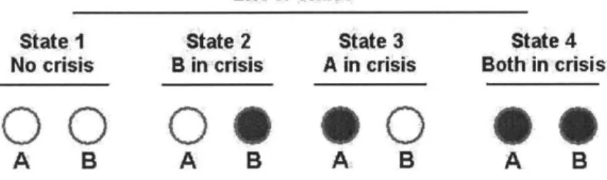
Each country is assumed to be in one of two states: tranquil or crisis. A state of the world then, is defined as any combination of the states of its constituent countries. Figure 3-3 illustrates the Markov states for a two country case. The dark circles represent countries in crisis and the empty circles represent countries that are tranquil.

List of states State 2 Stae 3 B in crisis A in crisis

0

0 00

A

B

A

B

0@

Figure 3-3: Markov States for Two Country Case

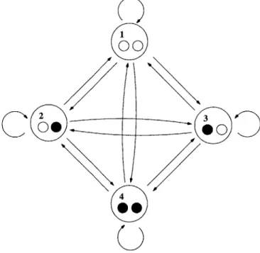
Figure 3-4 represents the Markov Chain for the two country case. Each circle rep-resents one state of the world. The arcs between circles represent the transitions from

'For a general treatment of Markov chains see Drake (1967).

State I No crisis

0 0

one state to another. Each of these arcs is associated with a transition probability of going from originating state to the terminating state.

1

00

00

@

00

Figure 3-4: Two Country Markov Chain

3.3

Mapping Global Relationships

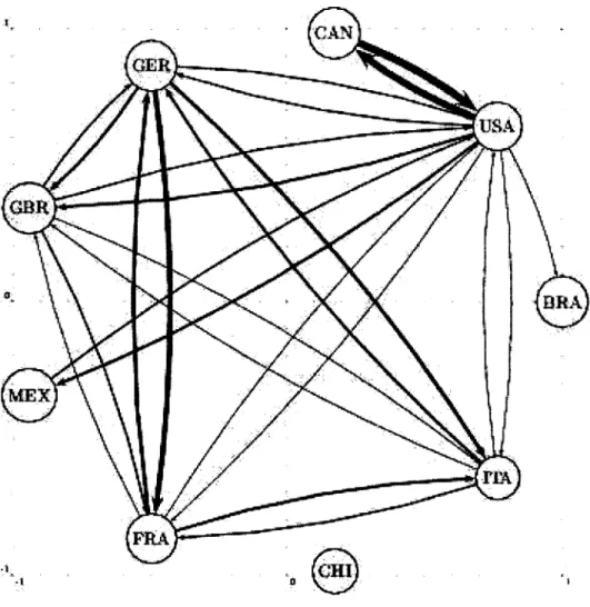
The next stage in modeling contagion involves mapping the dependencies between the countries under study. The dependencies are proxies for the channels through which crises spread from one country to another. The relationships between countries can be modeled as illustrated in figure 3-5 below. The world is represented as a directed graph in which each country is a node. Arcs represent relationships or dependencies between countries such that the thickness of each arc reflects the strength of the relationship or the magnitude of the dependency. A self loop represents a country's dependence on itself.

The model uses empirical data about countries to generate the Global Relationship Graph. The graph is represented in the model as a relationship matrix, R. This is an n x n matrix such that Rab is a non-negative number which shows the dependence

CAN USA 1R BRA MEX PRA

Figure 3-5: Global Relationship Graph for 9 countries: Canada, USA, Brazil, Italy, China, Fance, Mexico, United Kingdom, Germany

of country a on country b.

3.4

Generating Transition Probabilities

The final phase in modeling deals with generating transition probabilities between states in such a manner that the dependencies between countries are mapped appro-priately into the probability space. That is to say, if a country A is in crisis in state Si and country B has a high dependence on country A (as given in the relationship graph), then transitions to states in which country B is in crisis will have higher probability than states in which country B is not in crisis.

To generate a set of transition probabilities that satisfy the constraints of this system and preserve the relationship ordering a mathematical program is used. This model takes two inputs:

Global Relationship Graph: This is represented by the matrix, R, described above and represents beliefs about the contagion mechanism. Various channels of contagion can be used to generate this matrix.

[Unconditional

of contagion effects. An empirical estimate based on historical occurrences of crises is used for rk .

The output of the model is a matrix of transition probabilities for the Markov Chain formulation of the states of the world. The model is shown below.

Notation

Variables Description

Ak Country k

n Number of countries A1 through A, S Set of all possible states S1 through S2. pij Probability of transition from Si to Sj AC Event that country A is in crisis

A"' Event that country A is not in crisis i.e. is tranquil

Ij. Indicator variable

= 1 if Ak is in crisis in state Si = 0 otherwise

'rk unconditional crisis probability of Ak

Dki _{Dependence of country k on state i}

As shown above, the program requires the matrix D such that Dki is the depen-dence of country k on state i. In order to transform the relationship matrix into this state dependence matrix we perform the following calculation:

Rab R' b R= (3.2) Sb=1 Rab n Dki=

I 'R'

(3.3)

Intuitively, if each country is thought to have one unit of relationship to invest, then

Dki represents the amount of country k's relationship invested in crisis. The first step corresponds to normalizing each country's relationships to one unit. The second computes the amount invested in crisis.

Optimization Program

The objective function is chosen so as to make the unconditional crisis probabilities for each country predicted by the model as close as possible to the unconditional probabilities provided as inputs to the model. This ensures that the probabilities generated are consistent with empirically observed historical probabilities.

Minimize:

(P(

AC)

(3.4)

k=1

The program then specifies a set of Constraints to ensure that the probabilites generated are in accordance with probability laws and reflect beliefs about the

trans-mission of crises. The first constraint sets the bounds on the program variables pij. The [0,1] interval is mandated by the fact that they are probabilities.

0

P iPj

1

(3.5)

The next constraint is the total probability constraint stating that the sum of all outgoing probabilities from any Markov state should be one.

2"

Epi =

1

Vi

E

(3.6)

j=1

The next two constraints enforce the contagion effect. They ensure that the ordering of the countries in terms of the relative strength of their relationships is preserved.

(P(ACISj) - P(ACISj))(Dki - DkJ)

0

Vk

E

1..n,Vij E 1..2n

(3.7)

The first contagion constraint, shown above, preserves the ordering of crisis prob-abilities for one country starting from two different initial states. It ensures that if more of country k's relationships are invested in crisis in state Si than in Sj then it is more likely to go to crisis starting from the state Si than from Sj. This constraint ensures that the relationship ordering is preserved in the probabilities generated.

(P(ACISi)

-

P(ACISi))(Dki

-

D%) > 0

Vk,

1

E 1..n, Vi E 1..2n

(3.8)

The second contagion constraint preserves the ordering of crisis probabilities of two countries starting from the same initial state. It ensures that if country k has more of its relationships invested in crisis in state Si than country

1

1

The probabilities used in the constraints above are related by the following equa-tions, which are intermediate calculations to compute the value of P(AC) from the model variable pij.

P(AC) =

P(S)P(AfjSj)

Vk E

1..n

(3.9)

i=1 n

P(S)

E

k=1

P(ACISi)

=

E Ipij

Vk

e

1..n, Vi E 1..2"

(3.11)

jES

3.5

Analysis

The design goals against which the model should be assessed are: " Feasibility

" Computational tractability

e Optimality

The model's effectiveness can be gauged by it's ability to generate the desired state transition probabilities, and it's ability to reflect beliefs about the contagion mechanism in the probabilities generated. The analysis below demonstrates the exis-tence of a feasible solution for any instance of the model. To show that beliefs about contagion are adequately represented by the model, a simple theoretical instance of the model is solved analytically and intuitively.

3.5.1

Feasibility: Initial Feasible Solution

The model guarantees a feasible solution for any instance i.e. starting with any vector of unconditional default probabilities, ir, and non-negative relationship matrix, R.

Solution:

P(ACjSi)

We get:

n

ij=

H[Ik1P(A~ISj) +

Iki)(1

F(ACISi))]

Each Dki term is between 0 and 1 by construction (equations 3.2, 3.3). Since each of the terms in the product term defining pij is between 0 and 1, therefore the product must also be between 0 and 1. Hence constraint (3.5) is satisfied.

EjPij =

Z

H2=

[I P(AjSj) +

P(A

Ej

= 1

Intuitively, the above sum is 1 because it is equivalent to the sum of probabilities over all outcomes of an experiment in which k coins are tossed such that the probability that coin k will come up with heads is Dki. Hence the total probability constraint is satisfied.

The contagion constraints are also satisfied as shown below.

(P(ACISi)

P(Ai|Sj))(Dka

Dkj)

(Dk,

)

=

(Dki

(P(ACISi) - P(Af|Sj))(Dka - Di ) = (Dka - Di )(Ds - Di ) =

(Dki

Di

> 0

3.5.2

Optimality: Sanity Check

As a sanity check for the methodology, the model is compared against a scenario in which the expected solution is known or can be derived analytically. One such scenario is when each country is only dependent on itself. The matrix R is a diagonal matrix for instance the identity matrix, I. In this case, intuition suggests that in the optimal solution the state transition matrix should also be the identity matrix i.e. in the Markov chain, the self loops for each state have probability 1 and all other arcs have probability 0. Indeed, running the model on a diagonal matrix yields the

3.5.3

Tractability: Algorithmic Complexity, Runtime

The optimization formulated above is a quadratic programming problem. All the constraints are linear in the program variables and the objective is quadratic. The problem is solvable in polynomial time in the number of variables. However the number of variables is exponential in the number of countries. The current imple-mentation ran the problem on a 4 processor (Pentium III, 900 MHz) machine with 4 Gigabytes of memory for upto 8 countries. The program (using AMPL and LOQO) took about 3 hours to run.

3.6

Conditional Probability of a Crisis

If we are interested in the probability that a particular country develops a crisis within some time horizon, we can calculate the probability directly from the transition probability matrix. Let J represent the set of states where the country of interest is in crisis. In the two country example, country A is in crisis in state 3 and state 4. Then starting from state i, the probability that country A will be in crisis for the first time at time n, denoted

fi,

ff

= 0,

f=

1,p

C

JIXo

where i is an element of S. The probability of country A being in crisis within the next year starting from state i (where the time step in one month) is:

12

c =2

fi.

n=1

In order too calculate

fi,

\

example,

P11 P12 (3.16)

P21 P22_

We have dropped the columns and rows corresponding to states 3 and 4. The first transition probability becomes:

f= p'I Pn-2 , (3.17)

jEJ

where pi, and prj are vectors. The matrix P is raised to the power n - 2 because we are considering the probability of paths that enter the states represented by the reduced matrix on its first step, remain there for the next n - 2 steps, and enter one of the states in J on the final step.

Chapter 4

Model Instantiation

A particular instance of the model requires a choice of the relationship matrix, R,

and a choice of the unconditional crisis probabilities for each country, 7r. Together the choices represent beliefs about the world and the optimization program outputs will effectively model any system of such beliefs. The analysis presented here uses bilateral trade between countries as a proxy for the relationship matrix and computes the unconditional probabilities of crisis on the basis of historical values of Exchange Market Pressure.

4.0.1

Relationship Matrix: Bilateral Trade

The bilateral trade between any two countries is used to calculate the strength of the relationship i.e. the thickness of the arc. For the trade metric, R is defined as follows:

Rab = trade flow between country a and country b, when a

#

Rab = GDPa - EXPORTSa, when a = b

The trade flow is calculated as the sum of the exports and imports between the two countries.

4.0.2

Unconditional Crisis Probabilities

Currently the unconditional crisis probabilities are estimated using a historial measure of Exchange Market Pressure with a crisis threshold. Two methods of estimating the

probabilities are employed. The first uses a simple average of historical data and the second uses extremal value theory.

Exchange Market Pressure

The exchange market pressure index introduced by Eichengreen, Wyplosz, and Rose (1996) captures the notion of a currency crisis in a measure that can then be used to test for the explanatory power of macroeconomic variables. The EMP index incor-porates the three elements that are impacted by a speculative attack: the exchange rate, short-term interest rates, and central bank reserves. This chapter follows the version of the EMP used by Forbes (2001),

EMPk,t

+

y(%Arkt

%Arut)

(4.1)

where: ek,t denotes the price of U.S. dollars in country k's currency at time t; ik,t is country k's interest rate; iUt is the U.S. interest rate; ik,y is country k's interest rate calculated as a rolling average for the previous year starting at time t - 1, iuy,, is the U.S. interest rate calculated as a rolling average for the previous year starting at time t - 1; rk,t is the ratio of country k's international reserves to narrow money (Ml); rut is the ratio of international reserves to narrow money (MI) in the U.S. The weights a, , and -y are set to the inverse of the standard deviation for each series to equalize conditional volatilities. %A is measured as the weekly percentage log difference, for example,

%Aek,t = 100(ln ek,t - In ek,t_1)

To identify periods of crisis, a critical value of EMP for each is determined us-ing the mean and standard deviation of all EMP observations for that country. In particular, if

EMPk,t > /EMPk +± 3 EMPk, (4.2)

then country k is designated to be in crisis at time t, where pLEMPk is the mean of the EMP series for the country, and UEMPk is the standard deviation of the EMP series

for the country.

Extremal Value Theory

The probability of a crisis in a country can be obtained by dividing the number of crisis weeks by the total number of EMP observations. However, for countries that do not experience a crisis during the sample period, this value would be zero and imply that a crisis is impossible in these countries. Alternatively, to estimate the probability of crisis events, assume that the EMP of each country is a random variable with the right tail distributed according to the following extreme value distribution1

F(Xk) = 1 - DkX', Xk > 0, (4.3)

where Xk take on the EMP values of country k; ak is a parameter greater than zero to be estimated. We assume that Dk = U4k and that nk is equal to the sample mean

plus one sample standard deviation,

1

n

n

j

n(n - 1)

The cutoff, Uk, is chosen so that the density function is convex and thus better approximated by the extreme value distribution. Only EMP values for country k that are greater than the cutoff, Uk, are used to estimate the distribution. Hill's

maximum likelihood estimator of ak is (Embrechts, Kliippelberg, and Mikosch, 1997)

)-a= nU~ (4.5)

where the t values of Xj,k are greater than the cutoff, Uk. Estimate ak for each country

separately. Let

C

a crisis for country k is

t -ak.(4.6)U dkO Pk(Xk > =

1

where n is the number of observations in the EMP series.

When the historical measurement of crisis probabilities gives a non-zero value then that is used, otherwise extremal value calculations are used to estimate the crisis probabilities for the model.

Chapter 5

Results

5.1

Data

The information needed to calculate the bilateral trade matrix includes bilateral im-port and exim-port data between various pairs of countries. Direction of Trade Statistics (DOTS) provided by the IMF were used for this purpose. The data was located online at http://econ.bc.edu (restricted access website).

In order to calculate (Exchange Market Pressure) EMP values, we need data for the following:

" Foreign exchange rates to the dollar,

* Interest Rates,

" International Reserves

* Money Supply

In general, this data was collected from the International Financial Statistics Database available on CD-ROM. The time series ran monthly from January 1988 until December 2002. The detailed methodology is described below.

5.1.1

Trade Data

DOTS data was gathered for 44 countries including: Argentina, Australia, Austria, Belgium, Brazil, Canada, Chile, Colombia, Czech Republic, Denmark, Ecuador, Fin-land, France, Germany, Greece, Hong Kong, Hungary, India, Indonesia, IreFin-land, Is-rael, Italy, Japan, Korea, Malaysia, Mexico, Morocco, Netherlands, New Zealand, Norway, Peru, Philippines, Poland, Portugal, Russia (after 1996), Singapore, Slo-vak Republic, South Africa, Spain, Sweden, Switzerland, Thailand, the U.K., and Venezuela.

Data was collected between all sets of pairs of these countries (for instance Argentina-Australia, Argentina-Austria, Argentina-Belgium) for both imports and exports. The online data for imports was split into 2 groups: C.I.F. and F.O.B. 1 Data collected was from 1990-2002 and was sorted on a monthly basis.

GDP figures were used from the World Banks World Development Indicators database. For any given sample, the GDP figures from the year previous to the crisis year were used.

5.1.2

EMP Data

For the foreign exchange rates, IFS line "rf" was used in comparison to the US Dollar. This produces the average exchange rates on a monthly basis. Interest rates were taken from IFS line "60b". For countries where line "60b" did not produce a complete set of available data, then line "60" was used as a substitute. These interest rates produced end-of-month rates. Line 60b represents the money market rate and line 60 is the discount rate. An exception to this is Russia, where interest rates were available on Global Financial Database. Also note that before 1995, Russian interest rates were interpolated from quarterly numbers to get them in per month terms. International Reserves were found on IFS line "1L". These were end-of-month data. Money Supply was found on IFS line "34". These were also end-of-month data. An exception to this was the United Kingdom money supply, which was found on 'For more information about this online data source, please consult: http://fmwww.bc.edu/ec-p/data/DOTS.econ.html

datastream under the "MO" category.

5.2

Sample Results

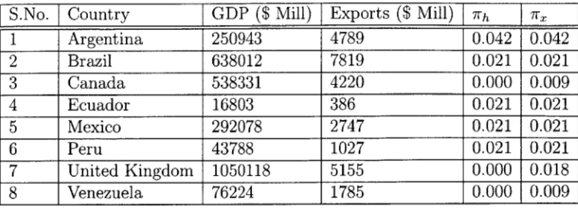
For empirical tests of the model six cases which correspond to historical crises were considered. The data was analyzed for these cases for groups of up to 8 countries each. The tables below show the model inputs calculated for each case. In each case data five years before the crisis month was used to construct the historical EMP values. The trade matrix was constructed using the preceding year's figures, as this was assumed to be the most accurate snapshot of the trade relationships before the crisis. The countries included and the time frame for each of the six cases are outlined below.

Case 1: Mexico Crisis, 1994 Argentina, Brazil, Canada, Ecuador, Mexico, Peru, United Kingdom, Venezuela

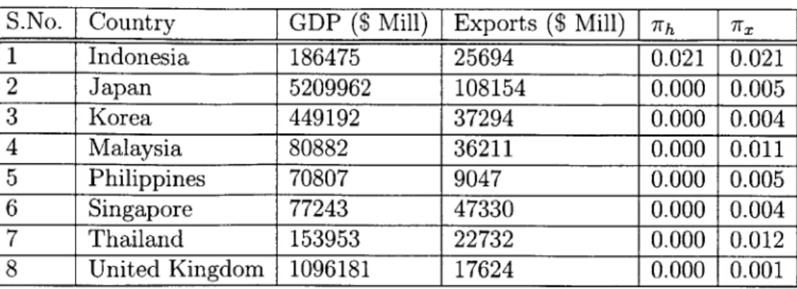
Case 2: Asia Crisis, 1997 Indonesia, Japan, Korea, Malaysia, Philippines, Singa-pore, Thailand, United Kingodom

Case 3: Russia Crisis, 1998 Indonesia, Malaysia, Thailand, Poland, Slovak Re-public, United Kingdom, Russia, Czech Republic

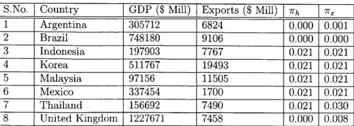
Case 4: Brazil Crisis, 1999 Argentina, Brazil, Indonesia, Korea, Malaysia, Mex-ico, Thailand, United Kingdom

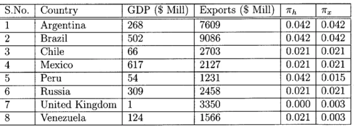
Case 5: Argentina Crisis, 2002 Argentina, Brazil, Chile, Mexico, Peru, Russia, United Kingdom, Venezuela

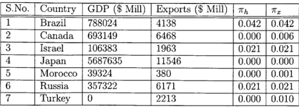
Case 6: Turkey Crisis, 2001 Brazil, Canada, Israel, Japan, Morocco, Russia, Turkey

The countries in each case were chosen so as to include major trading partners, countries to which crises spread and large countries as controls. 7rh indicates historical

Table 5.1: Sample Data for Case 1

S.No. Country GDP ($ Mill) I Exports ($ Mill) I 7h

],

1 Argentina 250943 4789 0.042 0.042 2 Brazil 638012 7819 0.021 0.021 3 Canada 538331 4220 0.000 0.009 4 Ecuador 16803 386 0.021 0.021 5 Mexico 292078 2747 0.021 0.021 6 Peru 43788 1027 0.021 0.021 7 United Kingdom 1050118 5155 0.000 0.018 8 Venezuela 76224 1785 0.000 0.009

Table 5.2: Sample Trade Data for Case 1

1

2

3

4

5

6

7

8

4 121

234

69

0

227

209 85

168

addition of crisis probabilities using the extremal value methodology for countries which showed 0 probability of crisis. The trade data is in millions of US dollars.

A sampling of the output of transition probabilites from the model is shown in the tables below. The contagion effects can be seen in the marked increase in crisis probabilities following a crisis in another country in the sample. The effect of the trade relationship can be seen in the relative magnitude of the crisis probabilities of two countries that are being affected by the country currently in crisis. In each case only two countries have been chosen for the purpose of illustration. For all but the Mexico crisis, the increase in probabilities and the ordering of probabilities between countries is consistent with expectations and in line with historical observations. In the case of the Mexico crisis, it is evident that trade is not an adequate channel for explaining the contagion mechanism. Figure 5-1 shows the crisis probabilities over

Table 5.3: Sample Data for Case 2

S.No.

I

I

Ji,

1 Indonesia 186475 25694 0.021 0.021 2 Japan 5209962 108154 0.000 0.005 3 Korea 449192 37294 0.000 0.004 4 Malaysia 80882 36211 0.000 0.011 5 Philippines 70807 9047 0.000 0.005 6 Singapore 77243 47330 0.000 0.004 7 Thailand 153953 22732 0.000 0.012 8 United Kingdom 1096181 17624 0.000 0.001

Table 5.4: Sample Trade Data for Case 2

1

2

3

4

5

6

7

8

6 0

32132 7832

41834 4932

0

12600 7890

time for Malaysia and Philippines. This is the probability that the country will go into crisis for the first time in the given period from the initial state. As can be seen from figure 5-1, the initial probability magnitude is closely tied to the difference in trade values, but subsequently the network effects in spreading the crisis dominate and both crisis probabilities converge.

5.3

Conclusion

The results of the analysis show that the model adequately replicates empirically observed crises in the data. It offers a general paradigm to model the dynamics of financial crises and is able to capture non-linearities in the spread of crises.

Malaysia

Philippines

3 4 1 1 7 1 9 ~I

Table 5.5: Sample Data for Case 3

S.No. Country GDP

($

1

Czech Republic

52036

5980

0.000 0.014

2

Indonesia

202132

6883

0.021

0.021

3

Malaysia

88832

8953

0.021

0.021

4

Poland

127085

4138

0.021 0.007

5

Russia

337709

8562

0.021 0.021

6

Slovak Republic

18377

3202

0.000 0.002

7

Thailand

168280

6381

0.021 0.021

8

United Kingdom 1126740

8985

0.000 0.006

Table 5.6: Sample Trade Data for Case 3

1

2

3

4

5

6

7

8

1

0

64

161

2560 2389 5093 84

2112

2

22

0

1985 117

155

10

1784 2063

3 34

2486 0

77

213

7

4576 3930

4 2485 212

216

0

3970 927

176

3403

5

1901

102

237

3205 0

1561 93

4132

6 4822 36

33

994

1702

0

24

459

7 0

1883 3978 123

104

0

0

2833

8

2173 2233 4435 3136 3975 298

2853 0

Table 5.7: Sample Data for Case 4

S.No. Country GDP

($

-

($

1

Argentina

305712

6824

0.000 0.001

2

Brazil

748180

9106

0.000 0.000

3

Indonesia

197903

7767

0.021 0.021

Table 5.8: Sample Trade Data for Case 4

1 0

11229 169

752

401

772

303

806

2

11758 0

357

1748 515

1747 326

2781

3

168

494

0

4650 1942 204

1746 1687

4 602

2119

6526 0

6803 2309 2803

6875

5 275

376

2988 5902 0

353

5225 4652

6 489

1641

372

3414 1135 0

515

1996

7 298

342

2077 2680 4636 436

4

2819

8 796

2827

2329 6247 4835

1604 2931

0

Table 5.9: Sample Data for Case 5

S.No.

[

Country

GDP ($ Mill) I Exports ($ Mill)

[

1

Argentina

268

7609

0.042 0.042

2

Brazil

502

9086

0.042 0.042

3

Chile

66

2703

0.021 0.021

4

Mexico

617

2127

0.021 0.021

5

Peru

54

1231

0.042 0.015

6

Russia

309

2458

0.021 0.021

7

United Kingdom

1

3350

0.000 0.003

8

Venezuela

124

1566

0.021 0.003

Table 5.10: Sample Trade Data for Case 5

1

2

3

4

5

6

7

8

1 0

8880 1993

179

151

621

231

174

2

8842 0

1482 613

125 1582 373 949

3 2158 1518

0

328

219 944

458 62

4 443

1697 979

572

137 0

215 115

5 218

379

551

336

195 228

0

14

6

156

840

59

70

142 90

41

0

7 378

2282 627

300

78

896

196

2891

8

170

837

255

1365

199 572

269 11

Table 5.11: Sample Data for Case 6

S.No.

I

($

($

1

Brazil

788024

4138

0.042 0.042

2

Canada

693149

6468

0.000 0.006

3

Israel

106383

1963

0.021 0.021

4

Japan

5687635

11546

0.000 0.000

5

Morocco

39324

380

0.000 0.001

6

Russia

357322

6171

0.021 0.021

7

Turkey

0

2213

0.000 0.010

Table 5.12: Sample Trade Data for Case 6

1

2

3

4

5

6

7

1

0

1575

594

5356

296 1613 208

2

1671

0

663

15691 228 441

291

3

514

573

0

1813

1

678

868

4 5018 14316

1767 0

413 4568 891

5

349

254

0

348

0

414

140

6 1108 300

500

3251

180 0

3313

7

321

352

1178 1472

145 3742

0

Table 5.13: Asian Crisis

Inital State: all tranquil Initial State: Thailand crisis

Malaysia

0.007

0.030

Philippines 0.007

0.018

Table 5.14: Russia Crisis

Inital State: all tranquil Initial State: Russia crisis

Czech Republic 0.009

0.165

Table 5.15: Turkey Crisis

Inital State: all tranquil Initial State: Turkey crisis

Israel 0.0118 0.0247

Russia 0.0089 0.0304

Table 5.16: Mexico Crisis

Inital State: all tranquil Initial State: Mexico crisis

Brazil 0.0066 0.0244

References

Baig, T. and Goldfajn, I., 1999, "Financial Market Contagion in the Asian Crisis." IMF Staff Papers, 46(2, June), pp. 167-195.

Calvo, G.A., 1998, "Capital Flows and Capital Market Crises: The Simple Eco-nomics of Sudden Stops." Journal of Applied EcoEco-nomics, Vol. 1, No. 1, Novem-ber, pp. 35-54.

Dornbusch, R., Park, Y.C., and Claessens, S., 2001, "Contagion: Why Crises Spread and How This Can Be Stopped." International Financial Contagion, pp. 19-41. Drake, A., 1967, Fundamentals of Applied Probability Theory, McGraw-Hill.

Eichengreen, B., Rose, A., and Wyplosz, C., 1996, "Contagious Currency Crises." National Bureau of Economic Research Working Paper, 5681.

Eichengreen, B.J., Rose, A., and Wyplosz, C.A., 1996, "Contagious Currency Crises: First Tests." Scandinavian Journal of Economics, 98, 463-484.

Embrechts, P., Kliippelberg, C., and Mikosch, T., 1997, Modelling Extremal Events, Springer.

Forbes, K.J., 2001, "Are Trade Linkages Important Determinants of Country Vul-nerability to Crises?" National Bureau of Economic Research Working Paper, 8194.

Forbes, K.J. and Rigobon R., 2001, "No Contagion, Only Interdependence: Mea-suring Stock Market Co-Movements." Journal of Finance.

Forbes, K.J. and Rigobon R., 2001, "Measuring Contagion: Conceptual and Empir-ical Issues." International Financial Contagion.

Gerlach, S. and Smets, F., 1995, "Contagious Speculative Attacks." European Jour-nal of Political Economy, 11(1, March), pp. 45-63.

Glick, R. and Rose, A., 1999, "Contagion and Trade: Why are Currency Crises Regional?" Journal of International Money and Finance, 18(4, August), pp.

603-617.

International Monetary Fund, 2001, Direction of Trade Statistics.

International Monetary Fund, 2002, International Financial Statistics, CD-ROM. Rigobon, R., 1999, "Does Contagion Exist?" The Investment Strategy Pack, Banking

Rigobon, R., 2000, "On the Measurement of the International Propagation of Shocks: Is the transmission stable?" MIT mirneo.

Rigobon, R., 2001, "Contagion: How to Measure It?" National Bureau of Economic Research Working Paper, 8118.