Design and implementation of safety control for a class of stochastic order preserving systems with application to collision avoidance near intersections

Design and Implementation of Safety Control for a

Class of Stochastic Order Preserving Systems with

Application to Collision Avoidance near

MASSACHUSETTS MNB11ITE

Intersections

by

OCT 16

2014

Mojtaba Forghani

_LIBRARIES

Submitted to the Department of Mechanical Engineering

in partial fulfillment of the requirements for the degree of

Master of Science in Mechanical Engineering

at the

MASSACHUSETTS INSTITUTE OF TECHNOLOGY

September 2014

@

Massachusetts Institute of Technology 2014. All rights reserved.

Signature redacted

A uthor ...

Department of Mechanical Engineering

I

August 25, 2014

Certified by...Signature

redacted

...

Domitilla Del Vecchio

Associate Professor

Thesis Supervisor

Signature redacted

Accepted by...

David E. Hardt

Professor of Mechanical Engineering Department

Head of Graduate Office

Design and Implementation of Safety Control for a Class of

Stochastic Order Preserving Systems with Application to

Collision Avoidance near Intersections

by

Mojtaba Forghani

Submitted to the Department of Mechanical Engineering on August 25, 2014, in partial fulfillment of the

requirements for the degree of

Master of Science in Mechanical Engineering

Abstract

In this thesis, we have designed and implemented a safety control system for collision avoidance near intersections. We have solved the corresponding control problems for a general class of systems that also includes the scenario of the two consecutive vehi-cles approaching an intersection, which leads to the design of the collision avoidance system. We have gathered the data of behavior of drivers as they approach intersec-tions and have built a stochastic model for that through an optimization problem. The model generates a non-deterministic profile for acceleration of a vehicle which is not equipped with the collision avoidance system and it is used to estimate and predict future stopping profiles of the vehicle in order to take the right control action for avoidance or mitigation of accidents. First we have verified the consistency of the theoretical model with its expected behavior after implementation and then we have implemented the control system on the Prius vehicle in collaboration with TTC (Toyota Technical Center), Ann Arbor, Michigan.

Thesis Supervisor: Domitilla Del Vecchio Title: Associate Professor

Acknowledgments

I would like to express my appreciation to my advisor Professor Del Vecchio for her priceless helps and continuous supports during my graduate study. I would like to thank her for her motivation, patience, encouragement and caring about the students and for teaching me how to do research and how to write my thesis. I am very glad that I could have the opportunity to work under her supervision.

I would also like to thank Dr. John Michael McNew and Dr. Derek Caveney at Toyota Technical Center (TTC), Ann Arbor, Michigan, for helping me to implement the system on the vehicle. I would like to express my gratitude to Dr. McNew for his invaluable helps during my attendance in Ann Arbor, summer 2013 and 2014.

I thank my friends at Professor Del Vecchio's research group, Control Networks Group. I am very thankful to Dr. Daniel Hoehener at Control Network Group for his helps and ideas. I also would like to thank the Graduate Office of MIT MechE.

My special thanks to my parents for all the helps, supports and sacrifices that

they have made for me. Words can never help me express how grateful I am for their encouragements and prayers, that despite the far distance between us, have always been a motivation for me.

I would also like to thank National Science Foundation (NSF) for supporting my work under the award number 1161893.

Contents

1 Introduction 9

1.1 General Collision Scenario . . . . 10

1.2 Related Works . . . .. . . . . 11

2 Deterministic vs Stochastic Systems 13 2.1 Deterministic System . . . . 13 2.2 Stochastic System . . . . 15 3 Stochastic Model 17 3.1 System Model . . . . 17 3.2 Motivating Example . . . . 20 3.3 Problem Formulation . . . . 27 3.4 Solution to Problem 1 . . . . 29 3.5 Solution to Problem 2 . . . . 37 3.6 Algorithms . . . . 38

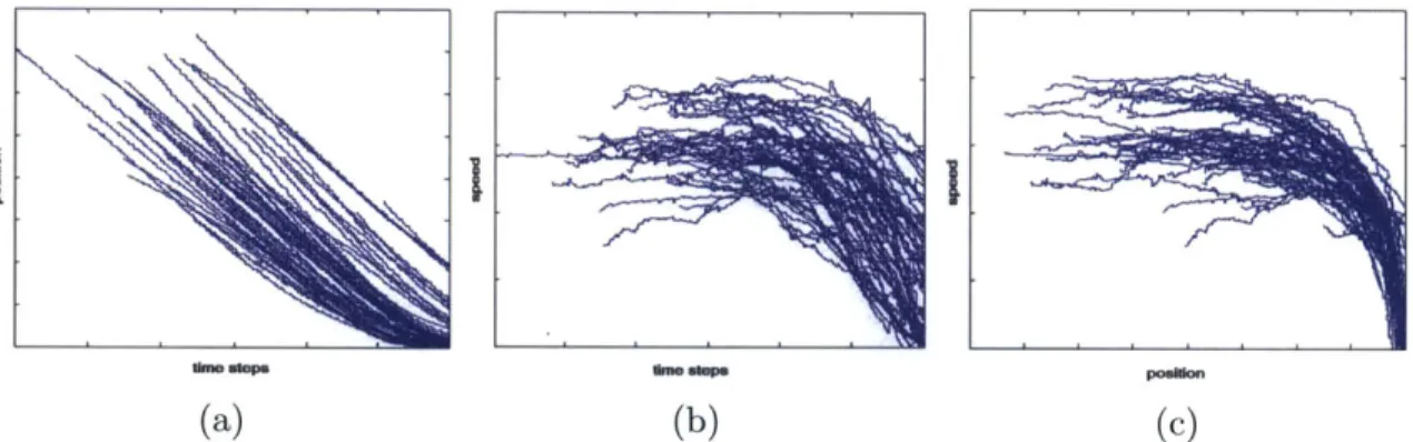
3.7 Simulations and Data Analysis . . . . 43

3.7.1 Experimental Setup . . . . 43

3.7.2 Experimental Results . . . . 45

Chapter 1

Introduction

The first recorded automobile fatality goes back to 1869 [1]. Today after almost 150 years, with the all developments in the safety technologies of vehicles, still number of injuries and deaths caused by automobile accidents is significant. In 2007 the contribution of intersection related crashes among all types of accidents was reported to be 40% [2]. Among all different possible intersection related crashes one is the rear-end collision that takes place between two vehicles in the same lane. Drivers may have wrong estimation of the decision that driver of their preceding vehicle is making or going to make and this can put both vehicles in the dangerous situation of rear-end collision. Obviously, a vehicle that is crossing an intersection with a high velocity (namely a velocity higher than a maximum value) is the source of a different type of collisions that occurs inside the intersection. Considering these two situations, we are interested in design of a semi-autonomous control system that helps the driver to avoid or mitigate collisions, with the basic assumption that only our vehicle is equipped with the collision avoidance system.

In Section 1.1 we provide more details of the general collision scenario that we are considering throughout the thesis and in Section 1.2 we review some of the related works regarding the collision prevention and mitigation.

1.1

General Collision Scenario

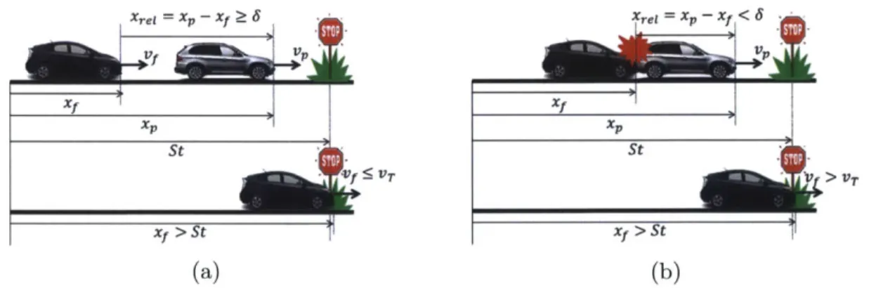
We denote longitudinal position and velocity of the preceding vehicle (PV), if it exists, by x, and v,, respectively. The position and the velocity of the following vehicle (FV), the vehicle that is equipped with the collision avoidance system, are Xf and Vf, respectively. The longitudinal position of the intersection (stop sign) is also denoted by St and the maximum allowable velocity (target velocity) is represented by

VT. The minimum allowable distance between the two vehicles is 6. Mathematically,

(1) xp - xf < 6 or (2) Vf > VTand xf > St, (1.1)

denotes the collision state. The scenario is depicted in Figure 1.1.

xx fs

(a) (b)

Figure 1.1: The collision is defined as (1)- If the distance between the two vehicles becomes smaller than 6, or (2)- If FV passes the intersection with a velocity larger than VT. In Figure (a) none of the two constraints are violated. In Figure (b), the top figure, the first constraint is violated, and in the bottom figure the second constraint is violated.

Since no collision avoidance system is implemented on PV, FV must be equipped with a control system that has a reasonable estimation of the current and future decisions of the driver of PV. Note that if any of the two constraints of equation (1.1) is satisfied, at any time, the system will be in the collision state, and since we do not have the information of the future states of PV and FV, the future estimation is essential in order to design the control system. In the next section we focus on different methods that have been employed for the estimation purposes.

1.2

Related Works

A popular tool to model a set of time series observations, which in our case is the past

behavior of drivers of PV as they approach intersections, e.g., x, and vP, collected offline, is Hidden Markov Model (HMM). This method has been employed for simi-lar driver behavior detection purposes in [1]-[11]. HMM captures different observed behaviors through hidden states that their nature is not necessarily clear to us, and consequently any of the hidden states affects the observation through multiple pa-rameters. Although HMM is a powerful tool for estimation of the current state of the system, but it is not good at long term predictions. The accurate predictions of future states of the system are very essential. These predictions must be sufficiently accurate in order that we can make the right decision based on what will happen in future up to almost 30 sec, as the approximate maximum duration that the vehicle is inside the intersection region. In general HMM constructs a model for the system based on the available data and it does not consider the dynamic of the system. This can make HMM a good choice for a highly unknown system, but we already know the full dynamic of model of the two vehicles approaching an intersection.

In [3], [12] and [13] multiple noise driven linear systems have been considered as different behaviors of drivers, which themselves are classified based on HMM. This model can tackle the problem of using HMM solely, regarding the prediction of the future behaviors, but this model does not capture the nature of the behavior of PV. The position and the velocity of PV are generated by its acceleration and that is also generated by a driver that even in his/her worst state he/she follows a set of logical behaviors. Therefore a noise driven model while adds complexity to the problem, it cannot capture the nature of PV well. Then the question is that "What is a good model?" We will answer this question in the next chapter.

Chapter 2

Deterministic vs Stochastic

Systems

Since we are interested in having an estimation of the future profile of PV, we need a model that outputs a profile until the intersection or until the time that FV stops. The models mentioned in Chapter 1 consist of the discrete states that estimate or predict the most probable action that the driver is making or going to make. These models do not output any profiles for PV and in particular its acceleration, which itself drives the velocity and the position of PV in turn. We present two approaches to the collision avoidance problem. In Section 2.1 we present the deterministic model, and in Section 2.2 we introduce the stochastic model.

2.1

Deterministic System

A simple solution to the estimation of the future decision of the driver of PV is to

consider a constant acceleration for it until any time that the vehicle stops or cross the intersection. Since we are considering a constant acceleration for PV, we use the term deterministic system for this model, versus the stochastic model in which we do not consider a unique constant acceleration for PV and instead we assume it to be a random variable. In order to guarantee that for the deterministic model none of the inequalities of relation (1.1) are satisfied, we must consider an acceleration

value for PV that minimizes the distance between the vehicles, or in other words puts the system in the most dangerous situation. If we can guarantee that the vehicles are safe from the collision for this worst case scenario, then they are also safe for any other inputs of the driver of PV. This acceleration value corresponds to the minimum acceleration that PV can achieve. The minimum acceleration in vehicles is generated by applying the maximum brake force, which can easily be provided for any vehicles. In the deterministic model we check whether the profile corresponding

to the minimum acceleration violates the constraint x, - xf ;> 1, and based on that

we decide what control input must be provided to FV in order to guarantee the rear-end collision avoidance. This method, in spite of being fast and simple, suffers big problems which makes it almost inapplicable, in particular for the semi-autonomous collision avoidance system.

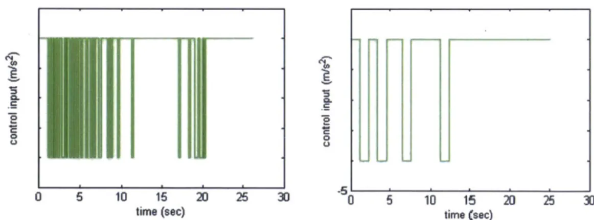
If we were confronting a fully autonomous control system, which in particular did not have human in the loop, we could take advantage of the deterministic system and guarantee that no collision will take place as long as the control system is operating properly. Existence of the driver of FV in the system (having human in the loop) does not allow us to design a system that always considers PV as an adversarial agent. While we are aware that the maximum brake or minimum acceleration is applied in rare situations, assuming that PV has always the minimum acceleration for the rest of its path leads to a very conservative system. Briefly, the deterministic system has two major problems; (1): It takes control action very early, meaning that from a considerably large distance to PV, which is not satisfactory for the driver of

FV; (2): Since the driver of PV rarely applies the maximum brake constantly, the frequency of the false alarms increases significantly, meaning that the number of the switches between the automatic control input and the driver input increases, which again leads to the dissatisfaction of the driver of FV. From the application point of view these two problems can make the model completely inapplicable and that is our main motivation for considering the stochastic system which does not suffer the above

'Note that the violation of this constraint means satisfying the first inequality of relation (1.1) which represents a collision state.

problems.

2.2

Stochastic System

The main difference between the deterministic system and the stochastic system is that in the stochastic system, unlike the deterministic system, the acceleration of PV is not assumed to always be its minimum possible value in order to estimate its future profile. Since the decision that the driver of PV makes is related to its current velocity and distance to the intersection2_{, we assume an acceleration as a function of}

the position and the velocity of the PV3. Moreover in order to capture the all possible different behaviors, we assume a Gaussian distribution around this function. The details of this model are provided in Chapter 3. With this model it is easier to relate the profile to a safety value. The major problem in the stochastic model is that we cannot guarantee 100% safety, and that is the reason that we have a safety level as an input to the stochastic system.

We use stochastic systems to mitigate the rear-end collision instead of completely preventing it from happening as we do in the deterministic model. The driver's satisfaction is the main reason for the transformation from the deterministic model to the stochastic model. In the next chapter, first we introduce a general class of systems and then prove that our collision avoidance scenario is also consistent with this class of systems, and then we solve the corresponding control problems regarding the expected safety of the model.

2

For instance when the speed is higher or the vehicle is closer to the stop sign, we expect a larger required deceleration in order to stop the vehicle at the intersection.

Chapter 3

Stochastic Model

In order to tackle the problems introduced in Chapter 2 regarding the conservativeness of the deterministic model, which itself leads to the dissatisfaction of the driver of FV, we take advantage of stochastic systems. In Chapter 3, we first introduce the new model in Section 3.1. In Section 3.2 we prove that the collision avoidance system can be modeled as a motivating example having the property of the class of systems considered in Section 3.1. We then formulate the problems that need to be solved based on the new model in Section 3.3. In Sections 3.4 and 3.5 we will solve the two problems mentioned in Section 3.3. In Section 3.6 we present the general algorithm to solve the relevant problems of Section 3.3, and we will introduce the discrete algorithm for implementation purposes. In the last section, Section 3.7, we will present simulation results along with the required ools to build the model from the available data.

3.1

System Model

Before introducing the model that we are considering, we define the strict and non-strict order preserving properties, which we will use extensively throughout this chap-ter.

a partial order relation "<", which we denote by the pair (P, 5). The partial order

(Rn, <) with component-wise ordering is defined as follows. For all w, z ( RE we have

that w < z if and only if wi zi for all i

E

component of w. We denote piecewise continuous signal on U by S(U) := PC(R+, U). With this notation, for U C R' we define the partial order (S(U), ) by component-wise ordering for all times, that is, for all w, z

E

E

Definition 2. A strict partial order is a set P with a partial order relation "< ", which

we denote by the pair (P, <). The partial order (Rn, <) with component-wise ordering is defined as follows. For all w, z

E

e

E

E

We consider a class of continuous systems that have some order preserving prop-erties.

Definition 3. A continuous system is a collection E = (X, U, A, 0, f, h), with state

x

E

E

E

y

E

Definition 4. For the systems E' = (X', U, A', 01,

f

= (X2 U2, A2, 02

,f2_{, h}2_{) we define the parallel composition E = El E2 := (X,U,A,0 f, h), in which}

X = X1 x X 2, U : XU 2, A:AXA 2, 0:=01 X0 2,f:=(f 1, f2) and hW:= (hd, h 2f

condition x E X, control input signal u E S(U) and disturbance input signal d E S(A). We also denote the ith component of the flow by q5 (t, x, u, d).

Definition 5. A continuous system E = (X, U, A, 0, f, h) is called input/output

order preserving (or strict order preserving) with respect to the control input, if the map h(q(t, x, u, d)) : U -+ 0 is an order preserving map (or strict order preserving map).

Definition 6. A continuous system E = (X, U, A, 0, f, h) is called input/output order preserving (or strict order preserving) with respect to the disturbance input, if the map h(O(t, x, u, d)) : A -+ 0 is an order preserving map (or strict order preserving map).

The system model that we are considering is defined as follows.

Definition 7. We consider the parallel composition of the systems E' = (X', U,

0,

c Rn

u E U = [UM, uM] C Rm with um E R' and uM E Rm, the minimal and the maximal control inputs for El, respectively, d E A = R, y' E 01, y2

E 02, h'(x') : X' 01

and h2_(x2_{) X}2 _{_+ 02. The vector fields are in the form of f 1(x',u) : X}1 _{x U -+X}

and f 2_(X2_{, d) : X}2 _{x A -+ X}2

.

We impose the order preserving properties on the flow of the system as follows.

Assumption 1. System El2 has input/output order preserving property with respect

to the control input.

Assumption 2. System EI2 has strict input/output order preserving property with

respect to the disturbance input.

Assumption 3. The disturbance input term of the system E2 is a constant

distur-bance input that can be modeled as a Gaussian distribution, that is d = d N(I, o2). We solve the corresponding control problems for the general class of systems in-troduced in this section, in Sections 3.4 and 3.5.

3.2

Motivating Example

Throughout this section first we model the scenario of the two vehicles approaching an intersection, and then we prove that it is consistent with the model that we have defined in Definition 7 and satisfies Assumptions 1-3. We denote the position and the speed of the following vehicle (FV) by Xf and Vf, respectively. Similarly the position and the speed of the preceding vehicle (PV) are represented by x, and Vp,

respectively. We denote the control input to the FV by u and the disturbance input term of PV by d. The deceleration due to the road load (rolling resistance) and the slope of the road on the FV are represented by a, and a, respectively, and the drag coefficient is denoted by C. We also impose a condition that the speed of both PV and FV must be non-negative. We use the superscript T to denote the transpose of a vector or matrix, e.g., AT represents the transpose of matrix A. The dimension of a vector space S is represented by dim S. Using these notations for the continuous form of the state space model of the system we have

x E X C R4_{, where x = (Xf,}

Vf , X,, V,)T, (3.1)

u E U c R, where U = {u I u E [um, u]}, (3.2)

d

E

f

f(x,

fl(x1 u){ f(xiu) if vf > 0 and 0 if Vf 0

f22 d) =. f ₍22_{, d) if v, > 0 (3.6)}

The functions f'(x', u) and f2(X2, d) are also in the following forms:

f'(x',u)= vand (2,d)= P (3.7)

U - CV2, - a,. - a, axp + bv, + d

The term ax,+ bvp+d is the acceleration of PV. We assume that d ~ N(p, O.2_{), which}

is consistent with Assumption 3.

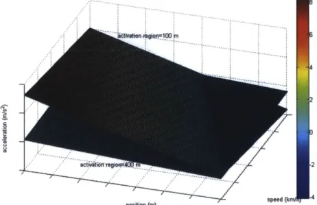
Since we cannot measure the acceleration of PV, we build a model that estimates it from the states of the system, the position and the speed. The parameters a, b,

p and a can be extracted through an optimization problem. More details of the

acceleration model along with the optimization problem will be provided in Section

3.7.

We can write (3.1)-(3.7) as the parallel composition of the two systems El

(X1,U, 0, 01, f1, h') and E2

(X 2, , A, 0 2_,

f 2_{, h}2_{), where x}1 _{= (xf, vf)T E X C R}2

and x2

= (xP,v,)T E X2 C R2_{, with X} = X1 xX2, u E U = [urn, uM] C R, d E A = R,

y =xf E R, y2 = x, E R, hl(x') = (1, 0)x' and h2(X2) = (1, 0)x2.The vector fields f'(x1 ,u) : x U -+ X1 and f 2₍₂2_{, d) :}

X2 X A -+ X2 _{will then take the forms}

f'(x1,)

f(x

0

jh

with fP(Xi, u) and f2_(X2_{, d) as defined in (3.7). This model is consistent with}

Defini-tion 7.

Since A' = 0 and U2 _{= 0, we represent flow of the systems El and}

E2 with

q1(t, x1, u) and

#

, d), respectively. Throughout the rest of this section we prove

that Assumptions 1 and 2 are valid for the scenario of two consecutive vehicles ap-proaching an intersection. Assumption 1 states that El must have input/output order preserving property with respect to the control input signal, meaning that

Xf(t) := h'(#1(t, x, u)) = 01(t, x, u) must be order preserving with respect to the

control input signal u. We prove that not only xf(t), but also Vf(t) := (t, x, u) has

order preserving property with respect to the control input signal. The order preserv-ing property of vf(t) is not necessary for consistency of the model with Definition 7, but it is required in order to satisfy another property that will be discussed in Section

3.3.

Proposition 1. The flows 1(t, x, u) = x1(t) and q1 (t, x, u) = vf(t) of the system

defined in (3.1)-(3.7) are order preserving with respect to-the control input signal u. Proof. If we consider two different control input signals ul and u2, such that ul > u2,

then for the velocity of PV at time t corresponding to these two control input signals, with the same initial conditions xf,l(O) = Xf,2(0) = x1(0) and vf,1(0) = Vf,2(O) = Vf (0), we have i'f,1(t) = ui(t)-CVj,1(t)2 _{-a,-aa and if,}

2(t) = u2(t)-CV 2 (t)-ar-a,

if both vf,1(t) > 0 and Vf,2(t) > 0. Let the function g(t) Vf,l(t) - Vf,2(t). At an

arbitrary time t we have

7(t)

= fn,1(t) - ')f,2(t) = (ui(t) - u₂(t)) - C (vf(t) - vf,2(t)) . (3.10)

Note that since we have chosen the same initial conditions, we have g(0) = vf,l(0) -vf,2(0) = 0. Because of the continuity of flow of the system with respect to time, if

order in state vf is not preserved, we must have a time t' E R+ such that g(t') = 0,

since otherwise for all t E R+, either g(t) < 0 or g(t) > 0. Therefore we can define

t* min{t E R+

I

0 and g(0) = g(t*) = 0, for the interval t E (0, t*) we have

NO)- lim g(h) - g(0) - lim g(h) >

h-+O+ h - 0 h-+o+ h since h > 0 : 3 h = hi E (0, t*) s.t. g(hi) > 0, (3.11) and similarly . g(t*) - g(t* + h) = g(t* + h) gt)= lim =-lim > 0 = h-+- t* - (t* + h) h-+0- h

since h < 0 : - h = h2 E (0, t*) s.t. g(h2) <0, (

and because of the continuity of the flow with respect to time, there is a t E [hi, h2]

such that g(t) = 0, which is in contradiction with the initial assumption that t*

min{t E R+

I

that Vf,l(t) > 0 and Vf,2(t) > 0 we have either g(t) = vf,1(t) - Vf,2(t) > 0 or g(t) = vf,1(t) - Vf,2(t) < 0. From (3.11) we conclude that the former is true.

We had assumed initially that vf,1(t) > 0 and Vf,2(t) > 0. For a case that for some

t' E R+ we have Vf,l(t') = 0 and vf,2(t') = 0, we let fi := min{t E R+ I Vf,1(t) = 0}

and f2 = min{t E R+

I

and vf,l(t) - Vf,2(t), we must have f2 < fl. If an arbitrary time t such that t E _{(0, t2),}

then g(t) = Vf,l(t) - Vf,2(t) > 0; If t E [f2, f4), then Vf,1(t) - Vf,2(t) = vf,i(t) > 0; And

if t E [f4, oo), then g(t) = Vf,l(t) - Vf,2(t) = 0. Therefore, in any case the order of

the flow of the velocity is preserved with respect to the control input signal. Since Xf,l(0) = Xf,2(0) = xf(0), then based on equation (3.7) Xf ,(t) - xf,2(t) = f g(s)ds >

0, which implies that the order preserving property of the flow of xf is also satisfied

with respect to the control input signal.

In Proposition 2 we will prove that Assumption 2 is also valid for our motivating

example, meaning that x,(t) h 2_(q2_{(t, x, d))}

=

#2

Proposition 2. For the system in the form of (3.1)-(3.7) the flow 2(t, x, d) x,(t)

is strictly order preserving with respect to d.

Proof. Let Xo := (xf,of,o, XO,, vp,o)T be the initial condition, where vf,O > 0 and

v,,o > 0. According to Assumption 3 we have d(t) = d where d ~ (p, a2_{). From}

equations (3.6) and (3.7) we have that the velocity of PV, for v,(t) > 0, satisfies the following differential equation:

VP - bp, - avp = 0 where v,(0) = v,,o and i),(0) = axp,o + bvp,o + d. (3.13) (3.12)

The above differential equation has the solution in the form

v,(t) = kieAlt

+

A, = 0.5(b +

V2

Vb2

Since complex and real values of A, and A₂ reveal different behaviors for vp(t), we consider different possible cases and analyze the behavior of xp(t) with respect to d for each of them. We divide the problem into three different cases; (1): b2 _{+ 4a > 0,}

(2): b2 _{+ 4a < 0 and (3): b}2 _{+ 4a = 0. For each case we consider two disturbance}

signals d' = d' and d2 _{= d}2 _{such that d' > d}2 _{and determine the relationship between}

v (t) and vj(t) and then between 1(t) and x4(t), the velocity and the position of PV at time t corresponding to d' and d2, respectively.

Case (1): If b2 _{+ 4a > 0, then A, and A}

2 in (3.14) are real numbers. The solution

of (3.13) then takes the form

v,(t ) = A((vpo( - b) - ax,o - d) e lt - (v,o(Al - b) - ax,O - d) e A2t)

(3.15)

If we replace d in equation (3.15) with d and d2 in order to obtain their corresponding velocities at time t, represented by vo(t) and v (t), respectively, we have

_,(t V2 v-(2t -=-_A () A (eA2t _ exlt). (3.16)

Note that (3.16) can become zero only when t = 0. Therefore because of the continuity of flow of the system with respect to time, for all t E R+, either v,1(t) - V (t) > 0 or vi(t) - v (t) < 0. To determine which of these two cases holds, we note that in general for any x E R - {0} we have that if x > 0, then ex - 1 > 0 and if x < 0, then e' - 1 < 0. These two statements together imply that '-I > 0. Since in Case (1) A2 - Al #A 0 and we are considering t E R+, then (A2 - Al)t

#

replace x with (A2- Al)t.

e(A2-A1)t - 1 e(A2-A1)t -

1

eA

-> 0 => te*lt > 0 => eAt > 0 =

(A2-~ d -j IdA-2jtIA2-A

d' - A2 (eA2t _ eXit) > 0 => V (t) > v (t), (3.17) where we have used the facts that t E R+, eAli > 0 and d' - d2 > 0. By integrating

both sides of (3.17) to determine the position of PV at time t, we obtain

t t

0vP (u) du > fov2 (u) du=

Xp,0 + tv,(u)du > xp,, +

j0

Case (2): If b2

₊

1 and A2 in (3.14) are complex numbers. The

solution of (3.13) then takes the form

vP() = eat (ax,o + (b - a)v,o+d s t + vO Cos

with a =.0.5b, and

#

If we replace d in equation (3.19) with d' and d2 _{in order to obtain their corresponding} velocities at time t, represented by v1(t) and vP (t), respectively, we have

ve (t) _ v(t) = d at sin ,t. (3.20)

We observe that in Case (2), unlike Case (1), we cannot guarantee that for all t E R+, v (t) - v2(t)

#

alternatively, 3t = k7r, for all k E Z. The smallest t E R+ that satisfies sin #t = 0 is

C* = 0. The velocity of PV at time V* corresponding to d' and d2, based on equation

(3.19), is given by

at* (3 a*

Since for all t E R+, vp(t) > 0, we must have vp'(t*) = 0, or in other words, for

all t E [0,tt*] we have either vp(t) - v2(t) > 0 or vp(t) - v2(t) < 0. In order to

determine which case holds, we note that for all t E [0, t*] we have

f

eat (d' - d2) > 0. These two statements along with (3.20) imply that v (t) -v,(t) > 0. Since in (3.19) we have VP(0) = v,,o > 0 and v2(t*) = -vp,oe*t* < 0, then because of

the continuity of flow of the system with respect to time, there is a f E (0, t*) such that f:= min{t E (0, t*) I v (t) = O}. Then we have for all t E (0,), v, (t) - v (t) > 0. For a t E (0, 0, we have

x (t) - x (t) = j(v(u) -

vp(u))du

For a t E [i, t*) we have

t t

x (t) - x (t) = (v, (u) - v (u))du + (v (u) - v (u))du >

0 + J(v (u) - v (u))du > 0 =>

4(t)

(t)

and for a t E [t*, oo), we have

X4(t) -

(t)

f(v

J;*

(v (u) - Vo(u))du + 0 > 0 => X (t) - X (t) > 0. (3.24)

Case (3): If b2 _{+ 4a = 0, then A, = A}

2 = A, which is also a real number. The

solution of (3.13) then takes the form

vp(t) = eA't [vp,o + (axp,o + (b - A)vp,o + d) t], (3.25)

and for v (t) - v2(t) we have

which implies

I(t)

4(t)

We had assumed initially that v (t) > 0 and v2(t) > 0. In general we may have a time t* such that v (t*) = 0 and v,2(t*) = 0. In this case, because of the

continuity of flow of the system with respect to time, there are times fi and f2 such

that fi = sup{t E (0, t*) I v, (t) > 0} and f2 = sup{t E (0, t*) | v (t) > 0}. Since we

have proved through Cases (1)-(3) that as long as vo(t) > 0 and v (t) > 0 we have v (t) - v2(t) > 0, then f2 < f. For an arbitrary time r E (0, f2) Cases (1)-(3) imply

that x (r) - x(r) > 0; If r E [2, [₁), then

x (r) - X (r) = (v (u) - v2(u))du + J(v (u) - 0)du > 0; (3.28)

And if T E [f, oo), then

, (r) - x

(r)

and the proof is complete. L

3.3

Problem Formulation

Before formulating the problem we define the bad set.

Definition 8. For a system with the states x E X, the bad set, B, is a subset of the space of the states, B C X, that the system should never enter, that is, for all

t E R+, x(t) B.

Because of the restrictions that we have on our control input, u E [um, UM] C Rm, there is no guarantee that if an initial state of the system is outside of the bad set, it will never enter it. Therefore we need to introduce a game between the control input and the disturbance input such that the probability that the control input wins, which means not entering the bad set, is a given value P. Our main goal is to design

a control strategy that guarantees success of the control input P% of the time. We use Pr(.) to denote the probability and p(.) to denote the probability density function. We represent signal of the states of the system by x E S(X), where X := X' x X2_.

We denote a static feedback map with 7r : X -+ U. With these notations, the flow of the system with feedback map 7r, initial condition x and disturbance signal d, is represented by

#(t,

Assumption 4. The bad set is in the form

B=U_1

{xEX

{xEX

I Ch

1_(x1_{) -} 2 _h2 2_{) > H}

_},

B1 B2

where C' and C2 are r x dim(01) and r x dim(02_{) matrices, respectively, with} ci,3,c?,3 0. hl(xl) and h2(x2) are as defined in Definition 7, H is a r-dimensional

vector, the functions Gj are such that Gi(x') : X -+ RP' and g9s are p3-dimensional vectors.

We impose one more assumption on function Gj before formulating the control problems.

Assumption 5. The map G(xl) = G3(q1(t, x1(0), u)) : U -+ RP!, for

E {1, ... ,N},

The two following problems concerned with the P% safety of the system intro-duced in Definition 7 must be solved.

Problem 1. For the system E = E1||E2, defined in Definition 7, with Assumptions

1-5 and P E (0,1), find the open loop maximal safe set given by

W := {x E X 13 u E S(U) s.t. Pr(#(t, x, u, d) V B, Vt E R+ and Vd E R) > P}.

1-5 and P

E

Pr(<b(t, x, u, d) B,Vt E R+ and Vd E R) > P where u= ir(x).

We have proved in Section 3.2 that the scenario of the two consecutive vehicles approaching an intersection is consistent with the system defined in Definition 7 and Assumptions 1-3. The bad set for the scenario of the two consecutive vehicles approaching an intersection, based on equation (1.1), is in the form

B = {x

E

B =

{x

E

I

I

B1 B2

for given St, VT and 6 representing the position of the intersection, the maximum allowable velocity at the intersection and the minimum allowable distance between vehicles, respectively. The set B1 corresponds to those states of the system that puts

FV at the intersection with a velocity higher than VT and the set B2 corresponds

to those states of the system that leads to collision between PV and FV. If we let C1 = C2 = 1, H = -6, G1(xl) = x1, g1 = (St, vT)T and N = 1, we observe that

the bad set can be written in the form assumed in Assumption 4. We have proved in Proposition 2 that the flows of xf and vf are order preserving with respect to the

control input signal, therefore since G'(x') = X1 = (x1, vf)T, Assumption 5 is also

valid for our motivating example. In the next two sections we will solve Problems 1 and 2.

3.4

Solution to Problem 1

Before proposing the solution to Problem 1 we need to define the capture set.

Definition 9. For the system defined in Definition 7, with Assumptions 1-5, the

states, x E X, defined as

C.(P) := {x E X I Pr((t, X, u, d) V B, Vt E R+ and Vd E R) < P}.

Lemma 1. The P-safety capture set of a given control input signal u E S(U), for

the bad set in the form of (3.30), can be written as

Cu(P) ={x E X I Pr (Vt E R+ and Vd E R,

C'h(#1(t, x1

,

U

Ix E X I 3t E R+, 3j E {l, ...,7 N} s.t. Gi (#1(t, x1 , u)) > gj

Proof. The bad set based on (3.30) is B = B1UB2. According to Definition 9 P-safety

capture set for input signal u for this bad set is

Cu(P) = {x E X I Pr (#(t, x, u, d) B1A

#(t, x, u, d) B2 , Vt E R+ and Vd E R) < P}. (3.32)

Let the set S be defined as

S := {x E X

I

#(t,x,u,d)

Ix E X I 3t E R+, 3j E {Il... N} s.t. Gj(# (t, x1, u)) > gi

}

We can rewrite (3.32) in the following form in which Sc {x E X

I

Cu(P) = {x E S U SC

I

V

Vt E R+ and Vd E R) < P} = {x E S

I

I

#(t, x, u, d) B2 , Vt E R+ and Vd E R)<P}. (3.

If x E S, since from Assumption 4 for all j E {1, ... , N} the function Gi is not function of the disturbance input d, then from (3.33) we have

Pr(#(t, x, u, d) ( B1, Vt E R+ and Vd E R) =

Pr(Vj E {1, ... , N}, Vt E R+, Gi(#(t, x, u)) < gi) = 0. _(3.35) Therefore if x E S, from (3.35) we have

Pr (#(t, x, u, d) B1 A #(t, x, u, d) B2, Vt E R+ and Vd E R) = 0 < P, (3.36)

which is true for all P E (0, 1). This implies that (3.34) can be written in the following

form:

C.(P) = S U {x E S'

I

0(t, x, u, d) B2, Vt E R+ and Vd E R) < P}.

If x E Sc, then from (3.33) we obtain

Pr(#(t, x, u, d) B1, Vt E R+ and Vd E R) = 1, (3.38)

which is independent of the event 0(t, x, u, d) E B2. This implies that if x E Sc, then

Pr (#(t, x, u, d) B₁ A #(t, x, u, d) V B2, Vt E R+ and Vd E R) =

Pr (#(t, x, u, d) ( B1, Vt E R+ and Vd E R) .Pr (#(t, x, u, d) B₂,

Vt E R+ and Vd E R) = Pr (O(t, x, u, d) V B2, Vt E R+ and Vd E R) , (3.39)

where to obtain the last equality we have used equation (3.38). From equations (3.37) and (3.39) we have

Cu(P) = S U {x E S

I

(3.34)

Since we know

{x E S

I

and S U S' = X, then we can write (3.40) in the form

Cu(P) = S U {x E X

I

If we replace S with its definition from (3.33) and use the definitions of B1 and B2 from (3.30), we can write equation (3.42) in the form of the statement of the Lemma. 13

Lemma 2. Let

Ftxu(d) := Clh'(q1(t,

and

(Ft",U)-'(s) := {d E R I Fj'x'u(d) = s}

with Ft,'U and (Fj'x')-1 denoting the ith component of Ftxu and (Ft*x'u)~,

respec-tively, and let the pair (t*, i*) (not necessarily unique) be

(t*, i*) = arg min Pr (Vd E R, d > (Fj'x)-1(Hj)),

VtER+ ViE{1,...,r} then we have

{x

+

(P))

Proof. Since based on Assumption 2 the function h2_(X2₎

= 42_{(t, x}2_{, d) is strictly}

order preserving with respect to d, then based on Assumption 4 C2_h2_(x2_{) is also}

strictly order preserving with respect to d and since h'(xl) is not function of d, then Ftx'u(d) = Clhl(xl) - C2_h2_(X2_{) is a strictly decreasing function of d and therefore}

invertible. Using this property we have

Pr (Vt E R+, Vd E R, C'h'(O'(t, x', u)) - C2h2(q2(t, x2, d)) H) =

Pr (Vt E R+, Vd E R, Fxu(d) H) =

Pr (Vt E R+, Vd E R, Vi E {1, ... , r}, Fxu(d) :H) = Pr (Vt E R+,Vd E R,Vi E {1, ... , r}, d > (Fit")- 1(Hi)) =

Pr (Vd E R, d > _{max (Fj'"tu)~1(H) =}

VtER+

min

VtER+ Pr (d E R, d > (Fit") 1 (Hi)) , (3.43)

ViE{1,...,r}

and using the definition of (t*, i*) we have

min Pr

(Vd

VtER+

ViE{1,...,r}

(3.44) In order to find a relationship between the disturbance input and the desired safety level P, we define the

Q

Q(z)

j

0

Since based on Assumption 3 d = d - N(p, a2), using

Q

we have that if Pr(Vd E R, d > (Fj>.*'')-1(Hi.)) < P, then

Q

)

01 (3.46)

Since Q(z) = 1 - _{4b(z) where 4 (z) represents the c.d.f. (cumulative distribution}

and also invertible. Therefore equation (3.46) can be written as (*''")-1(Hi*) _{- I > Q-}1_{(P) => (F''"x)-1}

(Hi.) > p + oQ'(P),

a s

and since FE.>''" is a strictly decreasing and invertible function, then Hi* < F.t*'XU(p

+

(P)),

(3.47)

(3.48)

and the proof is complete.

The following theorem provides a solution to Problem 1.

Theorem 1. For the system defined in Definition 7, with Assumptions 1-5, x E W

if and only if x 0 Cum(P).

Proof.

(<=)

Pr(#(t, x, um, d) V B, Vt E R+, Vd E R) > P, (3.49) which implies that x E W.

(=>) If x E W, then there is control input signal u' E S(U) such that Pr(#(t, x, u', d) ( B,Vt e R+,Vd e R) > P. If we replace the relation "<" in Definition 9 with the

relation ">" and use the results of Lemma 1 and Lemma 2, for x E W we have that there is control input signal u' E S(U) such that

Pr

(Vt

and Vt E R+,Vj E {1, ... , N} G3(# 1(t, x1, u')) gi. (3.50)

We prove that x C.m (P). Assume that by contradiction x E Cum (P), then we have Pr(#(t, x, um, d) B, Vt E R+, Vd E R) < P. Therefore x E Cum(P) based on Lemma 1 implies

(3.51)

or tER+,j E l, ... N} s.t. Gi(ma(t, x1, um)) > gi,

which based on Lemma 2 implies that

or 3t E R+, 3j E {1, ...,I _{N} SAt. Gi (0'(t, x', um)) > gi,} (3.52)

where

(t*,i*) = arg min

VtER+ ViE{1,...,r}

Pr

(Vd

If x E Cum(P), then based on equation (3.52) we can consider two cases. Case (1): Hj. < Fjt*,x,um(p + oQ-'(P)); Case (2): There is a time t E R+ and a j E

{1,) ...,I N} s.t. Gi (#1(t, x1,I um)) > gi

-Case (1): If x E W then according to (3.50) and Lemma 2 there is a control input signal u' E S(U) such that

Hit > F,'''U'(p + aQ 1(P)) where

(t', i') = arg min

VtER+

ViE{1,...,r}

Pr (Vd E _{Rd > (Ft"u')-1(Hi)) .}

Note that the pair (t*, i*) is not necessarily the same as (t', i'), but if Pr(d > (F,'')-(Hi)) P (which is equivalent to RI / > F,'' '"'(p + aQ-'(P)) based

on Lemma 2), then according to (3.54) we also have Pr(d > (F*',x'')-1(Hi*)) > P

(which is equivalent to H > F.*''"'(p

+

along with the equation Hj. < F.*,x,Um (p + aQ-1(P)), which is the main assumption

in Case 1, imply

+ aQ-(P)) <; H . < Fit.*:'(p + oQ-1(P)) =>

dim(Q') C*,k) dim(02 ) *j ,l h 02(* I2 -2 (3.53) (3.54)

dim(01) dim(02) Cl.,*khk(#1 (t*, X1, Um)) - c,h2 (2(t*2 ,2 , L + oQl(P))) k=1 1=1 dim(01) C .,k [h'(#1(t*, xl, u')) - h'(#1 (t*, xl, um))] < 0. (3.55) k=1

Since um is the minimal control input and based on Assumption 1 h' is an order preserving function of the control input signal u, then for all k E {1, ... , dim(01)} we have h)i(l(t*, 1, u')) - hh)(#1(t*, x1, um)) > 0. In turn, from Assumption 4 we have

that cij > 0. These two statements together contradict (3.55). Therefore we must have Hi. > Fb.*,xum(p _{+ OQ-1(P)).}

Case (2): If x E Cum(P), then we must have a time r E R+ and a j E {1, ... , N}

such that Gi (#1 (r, x1, um)) > gi. Because of the order preserving property of the

function Gi (q1 (r, x1_{, u)) with respect to the control input signal based on}

Assump-tion 5, for all u E S(U) we have G (01(r, x1, um)) Gi(1(-, x1, u)). Therefore if Gi (1(T, x1_{, um)) > gi, then we also have G (#1(r, x1, u)) > gi for all u E}

S(U). Since x E W, based on (3.50) there is also a control input signal u' E S(U) such tlhat

Vt E R+,Vj E {1, ... , N} : Gi(#1 (t, x1, u')) 5 g'. (3.56)

Since equation (3.56) is for all t E R+, then Gi(#1_{(r, x}1_{, u') 5 g}3_{, which}

contra-dicts our previous statement that for all control input signals u E S(U) we have G(1(r, x1, u)) > gi. Therefore there is no j E {1,...,N} and t E R+ such that Gi (1 (-r, x1, u)) > gi.

Since none of the assumptions of Case 1 or Case 2 are valid, then we must have

Hi. ;> F.*,xum(p + o-Q-1(P))

and

At

3.5

Solution to Problem 2

We consider the feedback control map

r(x)= U if x Cum(P)U .. OCum(P)

UM if x E Cum(P)U &Cum(P)

and state the following theorem.

Theorem 2. For the system defined in Definition 7, with Assumptions 1-5, for all

x

E

Proof. We consider two different cases.

Case (1): If for all t E R+ we have

#(t,

Case (2): If there is a time t* E R+ such that x(t*) =

#(t*,

I

#(f,

C = Cl(C) n Cl(Cc), where Cl(C) represents the closure of the set C, O(f, x, u, d) Cum (P),

#(t*,

#(t',

#(t',

I

#(,

OCum(P)-In order to guarantee that in Case (2) the control feedback map (3.58) provides the minimum P%, we divide Case (2) into two different subcases which we refer to as Subcase (2-a) and (2-b). In Subcase (2-a), for all t > f we have x(t) E Cum(P) U 9Cum(P). Therefore according to (3.58) for all t > i we have u(t) = um. Since x() = O(, x, u, d) 0 Cum(P), then we have Pr(#(t, x(), um, d) V B, Vt > f, Vd E R) > P

and for all t < f we have x(t) E W or alternatively Pr(#(t, x, u, d)

V

Therefore for the Subcase (2-a), the following control signal

U if t E [0,7t

ifte[O=)(39)

Uum) U if t E [f, oo)

will guarantee the minimum P% safety.

In Subcase (2-b), we assume that there is a t > f such that i inf{t E

(f, oo]

I

i

i

U if t E [0, 0~

u(t) um if t E [f,) (3.60)

U if t E [i, i)

Also for t > t we can divide the problem into two subcases as in Subcases (2-a) and

(2-b) and then we can guarantee that the minimum P% is satisfied.

3.6

Algorithms

In this section we propose the algorithms to calculate the control map suggested in Section 3.5.

Theorem 3. Let

dim(01) dim(02)

max Ckh1(#1(tx 1,um)) - ci,h2(#2_{(t, x}2_{,d)) - Hi (3.61)}