HAL Id: inserm-00517186
https://www.hal.inserm.fr/inserm-00517186
Submitted on 1 Aug 2011HAL is a multi-disciplinary open access archive for the deposit and dissemination of sci-entific research documents, whether they are pub-lished or not. The documents may come from teaching and research institutions in France or abroad, or from public or private research centers.
L’archive ouverte pluridisciplinaire HAL, est destinée au dépôt et à la diffusion de documents scientifiques de niveau recherche, publiés ou non, émanant des établissements d’enseignement et de recherche français ou étrangers, des laboratoires publics ou privés.
biophysical and statistical foundations.
Jean Daunizeau, Olivier David, Klaas Stephan
To cite this version:
Jean Daunizeau, Olivier David, Klaas Stephan. Dynamic causal modelling: a critical review of the biophysical and statistical foundations.. NeuroImage, Elsevier, 2011, 58 (2), pp.312-22. �10.1016/j.neuroimage.2009.11.062�. �inserm-00517186�
Dynamic Causal Modelling: a critical review
of the biophysical and statistical foundations
J. Daunizeau1,2, O. David3,4,5, K.E. Stephan1,2
1 Wellcome Trust Centre for Neuroimaging, University College of London, United Kingdom 2 Laboratory for Social and Neural Systems Research, Institute of Empirical Research in Economics,
University of Zurich, Switzerland
3 Inserm, U836, Grenoble Institut des Neurosciences, Grenoble, France
4 Université Joseph Fourier, Grenoble, France
5 Department of Neuroradiology and MRI unit, University Hospital, Grenoble France
Address for Correspondence Jean Daunizeau
Wellcome Trust Centre for Neuroimaging, Institute of Neurology, UCL
12 Queen Square, London, UK WC1N 3BG Tel (44) 207 833 7488
Fax (44) 207 813 1445
Abstract
The goal of Dynamic Causal Modelling (DCM) of neuroimaging data is to study experimentally induced changes in functional integration among brain regions. This requires (i) biophysically plausible and physiologically interpretable models of neuronal network dynamics that can predict distributed brain responses to experimental stimuli and (ii) efficient statistical methods for parameter estimation and model comparison. These two key components of DCM have been the focus of more than thirty methodological articles since the seminal work of Friston and colleagues published in 2003.
In this paper, we provide a critical review of the current state-of-the-art of DCM. We inspect the properties of DCM in relation to the most common neuroimaging modalities (fMRI and EEG/MEG) and the specificity of inference on neural systems that can be made from these data. We then discuss both the plausibility of the underlying biophysical models and the robustness of the statistical inversion techniques. Finally, we discuss potential extensions of the current DCM framework, such as stochastic DCMs, plastic DCMs and field DCMs.
1. Introduction
Neuroimaging studies of perception, cognition and action have traditionally focused on the
functional specialisation of individual areas for certain components of the processes of
interest (Friston 2002). Following a growing interest in contextual and extra-classical receptive fields effects in invasive electrophysiology (i.e. how the receptive fields of sensory neurons change according to context; Solomon et al. 2002), a similar shift has occurred in neuroimaging. It is now widely accepted that functional specialization can exhibit similar extra-classical phenomena; for example, the specialization of cortical areas may depend on the experimental context. These phenomena can be naturally explained in terms of functional
integration, which is mediated by context-dependent interactions among spatially segregated
areas (see, e.g., McIntosh 2000). In this view, the functional role played by any brain component (e.g. cortical area, sub-area, neuronal population or neuron) is defined largely by its connections (c.f. Passingham et al. 2002). In other terms, function emerges from the flow of information among brain areas. This has led many researchers to develop models and statistical methods for understanding brain connectivity. Three qualitatively different types of connectivity have been at the focus of attention (see e.g., Sporns 2007): (i) structural connectivity, (ii) functional connectivity and (iii) effective connectivity. Structural connectivity, i.e. the anatomical layout of axons and synaptic connections, determines which neural units interact directly with each other (Zeki and Shipp, 1988). Functional connectivity subsumes non-mechanistic (usually whole-brain) descriptions of statistical dependencies between measured time series (e.g., Greicus 2002). Lastly, effective connectivity refers to causal effects, i.e. the directed influence that system elements exert on each other (see Friston et al. 2007a for a comprehensive discussion).
This article is concerned with effective connectivity. It provides a critical review of Dynamic Causal Modelling (DCM), a relatively novel approach that was introduced in a seminal paper by Friston et al. 2003. The DCM framework has two main components: biophysical modelling and probabilistic statistical data analysis. Realistic neurobiological modelling is required to relate experimental manipulations (e.g., sensory stimulation, task demands) to observed brain network dynamics. However, highly context-dependent variables of these models cannot be known a priori, e.g., whether or not experimental manipulation did induce specific short-term plasticity. Therefore, statistical techniques (embedding the above biophysical models) are necessary for statistical inference on these context-dependent effects, which are the experimental questions of interest.
Taken together, these “two sides of the DCM coin” invite us to exploit biophysical quantitative knowledge to statistically assess context-specific effects of experimental manipulation onto brain dynamics and connectivity. This level of broad understanding of the DCM approach is tightly related to the mere definition of effective connectivity, in a physical and control theoretical sense. This also intuitively justifies why it might be argued that in its most generic form, DCM embraces most (if not all) effective connectivity analyses.
Nevertheless, existing implementations of DCM restrict the application of this generic perspective to more specific questions that are limited either by the unavoidable simplifying assumptions of the underlying biophysical models and/or by the bounded efficiency of the associated statistical inference techniques. This has motivated the development of many variants of DCM, focusing on either of the two DCM components. To date, about thirty DCM methodological articles have been published in the peer-reviewed literature. This makes them amenable to exhaustive reviewing, which we will expose in the first section of this article. In the second section, we will discuss the main criticisms that have (or could have) been raised against the existing DCM approach. Specifically, we will debate the plausibility of the underlying biophysical models, the robustness of the statistical inversion techniques and the practical issues related to its routine application. Finally, the third section discusses potential extensions of the current framework that address some of the issues discussed in this critical review and may further enhance the applicability and inferential power of DCM.
2. Dynamic Causal Modelling: review.
2.1. DCM: basics.
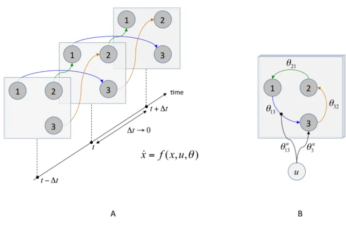
All variants of DCMs are based on so-called “generative models”, i.e. a quantitative description of the mechanisms by which observed data are generated. Typically, both hemodynamic (fMRI) and electromagnetic (EEG/MEG) signals arise from a network of functionally segregated sources, i.e. brain regions or neuronal populations. This network can be thought of as a directed graph, where sources correspond to nodes and conditional dependencies among the hidden states of each node are mediated by effective connectivity (edges). More precisely, DCMs are causal in at least two senses:
• DCMs describe how experimental manipulations ( ) influence the dynamics of hidden (neuronal) states of the system ( ), using ordinary differential equations (so-called evolution equations):
, (1)
where is the rate of change of the system’s states , summarizes the biophysical mechanisms underlying the temporal evolution of , and is a set of unknown evolution parameters. The structure of the evolution function determines both the presence/absence of edges in the graph and how these influence the dynamics of the system’s states (see Figure 1).
• DCMs map the system’s hidden states ( ) to experimental measures ( ). This is typically written as the following static observation equation:
, (2)
where is the instantaneous mapping from system states to observations, and is a set of unknown observation parameters.
This hierarchical chain of causality ( ) is critical for model inversion (i.e., estimation of unknown parameters and given ), since it (ideally) accounts for potential “spurious” covariations of measured time series that are due to the observation process (e.g. spatial mixing of sources at the level of the EEG/MEG sensors). This means that the neurobiological/biophysical validity of both the evolution ( ) and the observation ( ) functions is important for correctly identifying the presence/absence of the edges in the graph, i.e. the effective connectivity structure. We will refer to equations 1 and 2 as the “modelling component” of DCM.
The need for neurobiological plausibility can sometimes make DCMs fairly complex, at least compared to conventional regression-based models of effective connectivity, such as Structural Equation Modelling (SEM; McIntosh et al. 1994; Büchel & Friston 1997; Horwitz et al. 1999) or autoregressive models (Harrison et al. 2003; Roebroeck et al. 2005). This complexity, with potential non-identifiability problems, requires sophisticated model inversion techniques which are typically cast within a Bayesian framework:
• Using statistical assumptions about residual errors in the observation process, equations 1 and 2 are compiled to derive a likelihood function . This specifies how likely it is to observe a particular set of observations , given parameters of model .
• One defines priors on the model parameters which reflect knowledge about their likely range of values. Such priors can be (i) principled (e.g. certain parameters cannot have negative values), (ii) conservative (e.g. “shrinkage” priors that express the assumption that coupling parameters are zero), or (iii) empirical (based on previous, independent measurements).
• Combining the priors and the likelihood function allows one, via Bayes' Theorem, to derive both the marginal likelihood of the model (the so-called model evidence)
and e.g., an estimator of model parameters , through the posterior probability density function over :
, (4)
where the estimator is the first order moment of the posterior density1 (the
expected value of , given experimental data ).
The model evidence is used for model comparison (e.g., different network structures embedded in different evolution functions ). The posterior density is used for inference on model parameters (e.g., context-dependent modulation of effective connectivity). We will refer to equations 3 and 4 as the “statistical (or model inversion) component” of DCM.
This completes the description of the basic ingredients of the DCM framework. We now turn to the different variants of DCM for both fMRI and electrophysiological (EEG, MEG, LFP) data. Finally, we will examine the rationale behind the variational Bayesian method that is used to derive approximations to Eqs. 3 and 4.
2.2. DCM for fMRI
In fMRI, DCMs typically rely on two classes of states, namely “neuronal” and “hemodynamic” states. The latter encode the neurovascular coupling that is required to model variations in fMRI signals generated by neural activity.
In the seminal DCM article (Friston et al. 2003), the authors choose to reduce the “neuronal” evolution function to the most simple and generic form possible, i.e. a bilinear interaction between states and inputs . This form allows for quantitative inference on input-state and state-state (within-region) coupling parameters. Critically, it also enables one to infer on input-dependent state-state coupling modulation. This context-dependent modulation of
1 This estimator minimizes the expected sum of squared error . But other estimators could be
effective connectivity can be thought of as dynamic formulation of the so-called “psycho-physiological interactions” (Friston et al. 1997)2. The hemodynamic evolution function was
originally based on an extension of the so-called “Balloon model” (Buxton et al. 1998; Friston et al. 2000). In brief, neuronal state changes drive local changes in blood flow, which inflates blood volume and reduces deoxyhemoglobin content; the latter enter a (weakly) nonlinear . observation equation. This observation equation was subsequently modified to incorporate new knowledge on biophysical constants and account for MRI acquisition parameters, such as echo time (Stephan et al., 2007)and slice timing (Kiebel et al. 2007).
Two further extensions of the modelling component of DCM for fMRI data concerned the neuronal state equations. Marreiros et al. (2008a) adopted an extended neuronal model, with excitatory and inhibitory subpopulations in each region, allowing for an explicit description of intrinsic (between subpopulations) connectivity within a region. In addition, by using positivity constraints, the model reflects the fact that extrinsic (inter-regional) connections of cortical areas3 are purely excitatory (glutamatergic). Another approach by Stephan et al. 2008b
accounts for nonlinear interactions among synaptic inputs (e.g. by means of voltage-sensitive ion channels), where the effective strength of a connection between two regions is modulated by activity in a third region. Authors argue that this nonlinear gating of state-state coupling represent a key mechanism for various neurobiological processes, including top-down (e.g. attentional) modulation, learning and neuromodulation. The ensuing evolution function is quadratic in the states , where the quadratic gating terms act as “physio-physiological interactions”, effectively allowing one to specify the anatomical origin of context-dependent modulation of connectivity.
2.3. DCM for EEG/MEG/LFP
Biophysical models in DCMs for EEG/MEG/LFP data are typically considerably more complex than in DCMs for fMRI. This is because the exquisite richness in temporal information contained by electrophysiologically measured neuronal activity can only be captured by models that represent neurobiologically quite detailed mechanisms.
The DCM paper introducing DCM for EEG/MEG data (David et al. 2006) relied on a so-called “neural mass” model, whose explanatory power for induced and evoked responses had been
2 A comparison between dynamic (DCM) and static (SEM: structural equation modelling) effective connectivity
analyses can be found in Penny et al., 2004.
3 Regions of the basal ganglia and the brain stem have projection neurons that use inhibitory (GABA) and
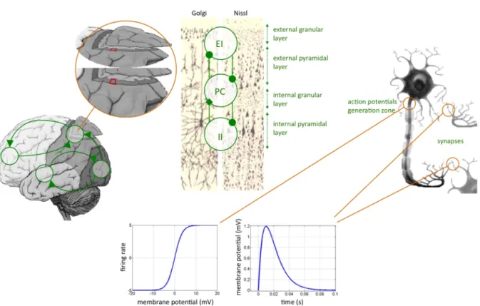
evaluated previously (David and Friston 2003, David et al. 2005). This model assumes that the dynamics of an ensemble of neurons (e.g., a cortical column) can be well approximated by its first order moment, i.e., the neural mass. Typically, the system’s states are the expected (over the ensemble) post-synaptic membrane depolarization and current. Each region is assumed to be composed of three interacting subpopulations (pyramidal cells, spiny-stellate excitatory and inhibitory interneurons) whose (fixed) intrinsic connectivity was derived from an invariant meso-scale cortical structure (Jansen and Rit, 1995). The evolution function of each subpopulation relies on two operators: a temporal convolution of the average presynaptic firing rate yielding the average postsynaptic membrane potential and an instantaneous sigmoidal mapping from membrane depolarization to firing rate4. Critically,
three qualitatively different extrinsinc (excitatory) connections types are considered (c.f.
Felleman and Van Essen 1991): (i) bottom-up or forward connections that originate in agranular layers and terminate in layer 4, (ii) top-down or backward connections that connect agranular layers and (iii) lateral connections that originate in agranular layers and target all layers (see Figure 2). Lastly, the observation function models the propagation of electromagnetic fields through head tissues (see e.g., Mosher et al. 1999). This “volume conduction” phenomenon is well known to result in a spatial mixing of the respective contributions of cortically segregated sources in the measured scalp EEG/MEG data5. This
forward model enables DCM to model differences in condition-specific evoked responses and explain them in terms of context-dependent modulation of connectivity (see e.g. Kiebel et al. 2007).
[Figure 2 about here]
Following the initial paper by David et al. (2006), a number of extensions to this “neural mass” DCM were proposed relating to both spatial and temporal aspects of MEG/EEG data. Concerning the spatial domain, one problem is that the position and extent of cortical sources are difficult to specify precisely a priori. Kiebel et al. 2006 proposed to estimate the positions and orientations of “equivalent current dipoles” (point representations of cortical sources) in addition to the evolution parameters . Fastenrath et al. 2008 introduce soft symmetry constraints which are useful to model bilateral homotopic sources. Daunizeau et al. 2009a included two sets of observation parameters : the unknown spatial profile of spatially extended cortical sources and the relative contribution of neural subpopulations
4Marreiros et al. 2008b interpret this sigmoid mapping as the consequence of the stochastic dispersion of
membrane depolarization (and action potential thresholds) within the neural ensemble.
within sources. With these extensions, DCM for EEG/MEG data can be considered a neurobiologically and biophysically informed source reconstruction method.
Concerning the temporal domain, computational problems can arise when dealing with recordings of enduring brain responses (e.g. trials extending over several seconds). In these cases it is more efficient to summarize the measured time series in terms of their spectral profile. This is the approach developed by Moran et al. (2007, 2008, 2009), which models local field potential (LFP) data based on the neural mass model described above, using a linearization of the evolution function around its steady-state (Moran et al. 2007). This approach is valid whenever brain activity can be assumed to consist of small perturbations around steady-state (background) activity. In Marreiros et al. 2008, the neural mass formulation was extended to second-order moments of neural ensemble dynamics, thereby enabling to model the dispersion over the ensembles. This mean-field6 formulation rests on
so-called “conductance-based” models a la Morris-Lecar (Moris & Lecar, 1981), which allow one to model gating effects at the neural ensemble level explicitly. Finally, David, 2007 proposed a phenomenological extension of DCM similar to the gating effects in the model by Stephan et al. 2008b. In brief, large-scale networks are thought to “self-organize” through a state-dependent modulation of the evolution parameters , which can change the structure of the attractor manifold of neural ensembles and induce dynamical bifurcations (c.f. Breakspear et al. 2005).
Beyond the neurophysiologically inspired formulations of DCM for electrophysiological data described above, two further DCM variants are noteworthy that rest on a more phenomenological perspective on EEG/MEG data. Chen et al. 2008 presented a DCM for so-called “induced responses”, i.e. a stimulus- or task-related increase in frequency-specific power of measured cortical activity. That is, both the data features and neuronal states are time series of power within frequency bands of interest. In this model, the emphasis is on linear versus nonlinear interactions among regions, which are expressed in terms of within-frequency and between-within-frequency couplings, respectively. Penny et al. 2009 extended the DCM framework to the analysis of phase-coupling, where the data features consist of narrowband filtered EEG/MEG measurements. In this work, the hidden states are the instantaneous phase of weakly coupled oscillators whose synchronization steady-state is (linearly) modulated by the experimental manipulation .
6 Mean-field theory originally derives from statistical physics. In our context, it consists of approximating the
interactions among all neurons within the ensemble by a (mean) field, thereby expressing the effective influence of the ensemble onto each of its members. Note that neural mass models are also derived from a mean-field treatment of ensemble dynamics (truncated to first-order moments of the ensemble density). See Harrison et al. 2005 for a seminal application of mean-field theory to conductance-based models of neural ensembles dynamics.
2.4. Approximate probabilistic (Bayesian) inference
According to equations 1 and 2, the measured data are a nonlinear function of unknown parameters , therefore the likelihood is not conjugate to the Gaussian priors on the parameters. This implies that the high-dimensional integrals required for Bayesian parameter estimation and model comparison (equations 3 and 4) cannot usually be evaluated analytically. Also, it is computationally very costly to evaluate them using numerical brute force or Monte-Carlo sampling schemes. This is the reason why the seminal DCM paper (Friston et al. 2003) introduced a variational Bayesian (VB) technique (c.f. Beal 2003). This method had previously been evaluated (c.f. Friston 2002) for the (weakly) nonlinear hemodynamic model that is used for the neuro-vascular coupling in DCM for fMRI (see section 2.2).
In brief, VB is an iterative algorithm that indirectly optimizes an approximation to both the model evidence and the posterior density . The key trick is to decompose the log model evidence into:
, (5)
where is any density over the model parameters, is the Kullback-Leibler divergence and the so-called free energy is defined as:
, (6)
where is the Shannon entropy of and the expectation is taken under . From equation 5, maximizing the functional with respect to indirectly minimizes the Kullback-Leibler divergence between and the exact posterior . This decomposition is complete in the sense that if , then .
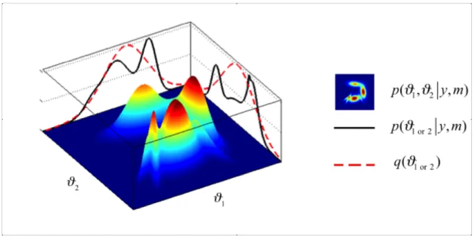
The iterative maximization of free energy is done under two simplifying assumptions about the functional form of , rendering an approximate posterior density over model parameters and an approximate log model evidence (see Figure 3):
• Posterior interactions between first-order moment parameters and second-order moment hyperparameters (e.g. the precision of the residual error in the observation process) are neglected. Consequently, factorizes into the product of the two marginal densities: . This assumption of “mean-field” separability is also implicit in the celebrated “Expectation-Maximization” (EM) algorithm (Yedidia 2000).
• The approximate marginal posterior densities above have a Gaussian fixed form. In turn, the first two moments (mean and covariance) of the (potentially multimodal) exact posterior density will be matched with those of the approximate marginal densities above (Figure 3). This is referred to as the “Laplace approximation” (see Friston et al. 2007b for full details) and the moments are called sufficient statistics, since they completely parameterize the approximate density.
The ensuing VB algorithm is amenable to semi-analytical treatment (the free energy optimization is made with respect to the sufficient statistics), which makes it generic, quick and efficient.
[Figure 3 about here]
Critically, no major improvement of the above VB framework was proposed so far. The main complementary statistical contribution has been dealing with the issue of Bayesian model comparison for group studies7. More precisely, Stephan and collaborators (Stephan et al.
2009) propose an additional VB algorithm addressing random effects at the between-subjects level, i.e. accounting for group heterogeneity or outliers. This second-level analysis provides the posterior probability of each model and a so-called “exceedance probability” of one model being more likely than any other model, given the group data. It also introduced model space partitioning, which allows one to compare subsets of all models considered, integrating out uncertainty about any aspect of model structure other than the one of interest. Penny et al. (submitted) extended this work to allow for comparisons between model families of arbitrary size and for Bayesian model averaging within model families.
2.5. Summary
Taken together, these contributions allow for statistical inference on context-specific modulation of effective connectivity, based on biophysically informed models of macro-scale neuronal dynamics. Both components of DCM rely on specific assumptions that may or may not be violated when analysing empirical data. In the following, we review the main criticisms that have (or could have) been levelled against DCM and its underlying assumptions.
3. Dynamic Causal Modelling: criticisms.
3.1. Plausibility of the biophysical modelling
Neuroanatomical and neurophysiological studies have been crucial in motivating the basic modelling assumptions that underlie DCMs for fMRI and electrophysiological data (for references, see the original DCM papers). However, one may question whether all neurobiological facts relevant for explaining neuronal population dynamics are already represented by existing DCMs. This question is of particular importance for DCMs of electrophysiological data, which have much more fine-grained representations of neuronal mechanisms than DCM for fMRI.
For example, macro-scale propagation effects, mediated by distance-dependent lateral connections, have not been properly accounted for8. These effects can be thought of as wave propagation in a complex medium, leading to spatiotemporal pattern formation or self-organization. Since the early work by Amari (Amari 1977), much effort has been invested in developing a neural field theory (e.g., see Deco et al. 2008 and references therein); incorporating these ideas into the DCM framework may prove fruitful.
Also, it is well known that neurons are subject to internal (e.g., thermal) noise, which may still have an impact at the population scale (see e.g., Soula and Chow, 2007 for “finite size” effects). If this is the case, the neural ensemble dynamics would deviate from the mean-field theoretical treatment that underlies most current modelling efforts in macro-scale neural dynamics (including DCMs).
Perhaps most importantly, there are several neurophysiological processes at the micro-scale that have been neglected in the current DCMs, including:
• Activity-dependent plasticity, i.e. continuously modified activity-dependent efficacy of synaptic transmission. These include different forms of short-term plasticity, such as synaptic depression/facilitation or spike-timing dependent plasticity, and long-term plasticity, such as long-term potentiation (LTP)- and depression (LTD).
• Dendritic backpropagation, i.e. the backpropagation of action potentials from the axon hillock back to the end of the dendritic tree (through active sodium conductances and voltage-gated calcium channels, which are not activated by normal excitatory postsynaptic potentials). This mechanism might be important for various phenomena, such as Hebbian-like learning, dendro-dendritic inhibition and conditional axonal output (Magee & Johnston 1997; Larkum et al. 2005; London & Häusser 2004). An important task for the future will be to evaluate whether the above processes are necessary for explaining neuronal population dynamics as observed with presently available recording techniques, and whether their parameters can actually be identified from the data. Concerning DCM for fMRI, the above phenomena are not explicitly modelled9. This may (or
may not) be a lesser concern as for electrophysiological DCMs, since it is unlikely that these fine-grained mechanisms are accurately reflected in and can be inferred from BOLD data. Instead, physiological details of the neuro-vascular coupling are perhaps more important (see Stephan et al. 2004 for review). So far, it neglects the potential influence of inhibitory activity on the hemodynamic response, which is a likely explanation for deactivations (Sotero and Trujillo, 2007; Shmuel et al. 2006). Furthermore, there is no realistic account of the metabolic cascade that relates synaptic activity and neuronal metabolism to the vasodilatation kinetics (Riera et al. 2006). This is mainly due to the simplistic account of neuronal activity in DCMs for fMRI, which does not disambiguate between e.g., postsynaptic membrane depolarization and presynaptic firing rate. Also, DCM for fMRI has also ignored the important role of glial cells (Takano et al., 2006; Iadecola & Nedergaard, 2007). Finally, a possible extension of the biophysical forward model in DCM is to take into account task-related physiological influences, e.g. of an endocrine, peripheral-autonomic or neuromodulotory sort (see Gray et al., 2009 for a review and Reyt et al., submitted for a first experimental description of this issue in the context of DCM).
Clearly, given the complexity of the models and the range of additional physiological mechanisms that may yet have to be accounted for, validation is an important issue for DCM
9 But see David 2007 & 2008 and Stephan et al, 2008b for phenomenological accounts of activity-dependent
(as for any other model of neuroimaging data). Simulations and experimental studies in humans and animals have been performed to address the reliability (Schuyler et al. 2009), face validity (e.g. Friston et al. 2003, Stephan et al. 2008b), construct validity (e.g. Penny et al. 2004a) and predictive validity (David et al. 2008; Moran et al. 2008) of different DCMs. Arguably, the hardest, but also most important challenge is to establish predictive validity. Animal studies will be indispensable for this task. For example, Moran et al. (2008) demonstrated that a DCM of steady-state electrophysiological responses correctly inferred changes in synaptic physiology, following a neurochemical manipulation, which were predicted from concurrent microdialysis measurements. In a next step, ongoing rodent studies test whether DCMs can infer selective changes in specific neuronal mechanisms that result from controlled experimental manipulations; e.g. changes in synaptic plasticity and spike-frequency adaption following application of both agonists and antagonists of the same transmitter receptor.
Perhaps the most far-reaching experimental assessment of the validity of DCM analyses so far was done by David et al. (2008), who performed concurrent fMRI and intracerebral EEG measurements to measure the spread of excitation in a genetically defined type of epilepsy in rodents. This study was the starting point for a methodological discussion, resulting in a series of articles in this issue (see the companion papers by Roebroeck et al. and Friston and Valdes). In brief, the study by David et al. (2008) (i) provides supportive evidence for the validity of DCM for inferring network structure from fMRI data and (ii) stresses the importance of having a model of neurovascular coupling. Clearly, this preliminary validation of DCM for fMRI is not fully sufficient and further dedicated experimental studies will be needed. Further invasive in vivo measurements of electrical (e.g. implantable miniaturized probes) and optical (e.g. two-photon laser scanning microscopy) signals are likely to be very useful for such an experimental validation (Riera et al., 2008).
3.2. Robustness of the statistical inference techniques
Criticisms can also be raised against the statistical component of DCM, which we will categorize into two subgroups, namely “frequentist” and “technical” criticisms. We will quickly address the former (which might have arisen from a misunderstanding of the Bayesian framework) and then focus on the latter (which are valid).
• It has been argued that both the number of parameters and the complexity of the models prevent any robust parameter estimation. Within a Bayesian framework, the role of the priors is to regularize or finesse the “ill-posedness” of the inverse problem. Informative priors basically reduce the effective degrees of freedom by constraining the parameters within a plausible range. This means that it is always possible to quantify the plausibility of any parameter value, given the data (i.e. the posterior density). If two parameters are redundant (as they have similar effects on the data), then they will have a high posterior covariance, which signals a non-identifiability issue. In turn, the model evidence diminishes towards zero10. This is important, since
such a model will be penalized for being non-identifiable, when compared with a simpler model (that is more identifiable).
• It has been argued that the proposed statistical framework cannot be used to formally test DCMs, in the sense that it cannot falsify them. Within a Bayesian framework, model comparison is formally a relative falsification approach, whereby less likely models are rejected against a more plausible one (given the data ). In other words, rather than testing against the (improbable) null hypothesis, the Bayesian formalism invites us to compare an arbitrarily large set of potentially plausible models (of relatively similar a priori plausibility). To relate this to the first point, a non-identifiability issue can (and should) cause the (relative) falsification (c.f. “Occam’s razor”).
• It has been argued that selecting a model based on the model evidence does not ensure that it has the greatest generalizability (as measured by e.g., cross-validation techniques). Within a Bayesian framework, models are compared on the basis of their plausibility, given all available data. Using informative priors actually prevents
overfitting (i.e. fitting the noise), which is the cause of incorrect predictions on yet
unobserved data. Furthermore, while a mathematically formal relationship between model evidence and generalisation error has yet to be established, previous studies have demonstrated a close correlation between the two indices (e.g. MacKay 1992). Beyond these general criticisms of Bayesian approaches, “technical” (but founded) concerns can be raised specifically against the variational Bayesian scheme that is used to derive approximate Bayesian inference.
First of all, the free energy optimization might be difficult, because the free energy itself can have multiple local maxima. This is important, since a local optimization scheme could
10 This is because the entropy term in the decomposition of the log model evidence (see equations 5 and 6) grows
unpredictably bias both the approximate posterior density and the approximate model evidence. In turn, this could be manifest as inconsistent parameter estimations and model comparisons across a set of repeated experiments (e.g. across trials or subjects). Several experimental studies have provided an experimental validation of the reproducibility of DCM inference within (Schuyler et al. 2009) or across subjects (Garrido et al., 2007, David et al., 2008 and Reyt et al., submitted). Nevertheless, the significance of this potential local optima issue has not been extensively assessed so far. Critically, the choice of the priors may drastically change the landscape of the free energy: more informative priors will dampen the local maxima that are away from the a priori plausible regions. This is important, since the free energy landscape determines the convergence of the free energy optimization scheme11. For example, updating the parameters of the evolution function (from their prior to their posterior expectation) might induce a bifurcation, i.e. a qualitative change in the dynamics of the system’s states . If this is the case, then the iterative update of the free energy will also experience a bifurcation, which may or may not confound the optimization scheme. Taken together, these potential concerns suggest that a thorough analysis of the free energy optimization procedure would be useful, in relation to both the dynamical repertoire of the modelled systems and the choice of the priors.
Second, even when the global maximum of the free energy is reached, a risk of biased inference still remains, due to the approximations in the posterior density (see section 2.4). For simple generative models12, it is known that VB approximate posterior densities have a
bias towards overconfidence (c.f. Beal 2003), i.e. VB posterior confidence intervals are correctly centred, but are too tight13. However, the presence of nonlinearities in either the
evolution ( ) or the observation ( ) function significantly changes the original VB tendency to be overconfident (Daunizeau et al., 2009b)14. Chumbley et al. 2007 validated posterior
confidence intervals on low-dimensional parameter vectors obtained with the above VB scheme, by comparing them to those derived from standard sampling schemes. This investigation gave reassuring results in that DCM parameter estimation was not significantly compromised by the (potentially crude) mean-field/Laplace approximation. However, one might still wonder how much model comparison based on a lower bound to the model
11 For example, the Newton optimization scheme can enter limit cycles if the iterative updates bounce between
different local maxima.
12 That is, models belonging to the exponential family.
13 This is because the mean-field approximation neglects probabilistic dependencies between sets of model
parameters.
evidence15 (and not on the model evidence per se) can be trusted. From equation 5, it can be
seen that the tightness of the bound scales with the statistical resemblance between the true and the approximate posterior densities. Therefore, the mean-field/Laplace approximation might be more problematic for model comparison than for parameter estimation. An informal consensus in the machine learning community is that VB algorithms should be numerically evaluated (using both simulated and real data) for each class of generative models. For DCMs, this extensive evaluation currently proceeds by the progressive accumulation of methodological and experimental studies.
Altogether, these properties of the variational Bayesian approach make it potentially sensitive to the above “frequentist” concerns. Model identifiability is such a subtle issue. Consider the case where (partial) parameter redundancy is common to all compared models (as, e.g., arising from the neurovascular coupling in DCM for fMRI, see Stephan et al., 2007). In this situation, the entropy term in Eq. 6 might dominate (see footnote 11). As a consequence, model comparisons might become inconclusive (no pronounced difference in the log model evidences). This means that parameter identifiability issues could potentially impact on model identifiability, and, in turn, lead to an overly conservative assessment of model generalizability. The situation would be different if the free energy was computed without the mean-field/Laplace approximation. This is because more global forms of posterior uncertainty could be accounted for (e.g., monomodal versus multimodal posterior densities), which would increase the statistical efficiency of model comparison.
Considering the potential problems discussed above, one might suggest using an “exact” sampling scheme instead of a VB algorithm. Theoretically indeed, this would be an acceptable solution, had the numerical curse of dimensionality16 no practical implications
whatsoever. But actually, experimental DCM studies now typically involve comparing a few hundreds models. In the case of inverting a relatively sparse DCM with, say, four regions, VB optimizes about four hundred (scalar) sufficient statistics to approximate the joint posterior density17. In comparison, a sampling algorithm would require approximately 1040
samples to represent it.
15 In DCM, the evaluation of the free energy under the mean-field/Laplace approximation is itself approximated
using a third-order truncation of the expectations involved (see e.g., Friston et al., 2007b). The resulting value for the free energy might not be a lower bound to the free energy. However, this says nothing about the tightness of the approximation.
16 If it takes n samples or bins to correctly represent a 1-dimensional probability density function, then it takes nd samples or bins to represent a d-dimensional density.
3.3. Practical issues
In addition to the potential modelling and statistical concerns above, a DCM user will face many practical issues. Here, we summarize only some of the most crucial conceptual points; for more details, see Stephan et al. (in press).
In a nutshell, DCM requires the scientist to make two choices: an experimental design for measuring brain responses and a set of alternative models for explaining these data.
A question frequently encountered in practice is whether there exists a way to optimize the experimental design for a DCM study. Theoretically, the answer is yes: (i) define the question of interest in terms of a model comparison problem and (ii) choose an experimental paradigm that maximizes the discriminability between the different models in . The first step is particularly important: it stresses that good experiments should enable one to decide between competing hypotheses and thus models. It also highlights that DCM is not a tool for exploratory analyses of data; even when hundreds or thousands of models are compared, the dimensions of model space are always related to a priori hypotheses about which neuronal populations and which mechanisms are important for explaining the phenomenon of interest. Concerning the second step, statistical approaches for solving this problem are conceivable, but are still under development (Daunizeau et al., in preparation).
Choosing the model set in a principled and hypothesis-driven way is crucial because any inference on model structure, via model comparison, depends on (c.f. Rudrauf et al., 2008; Stephan et al. 2009). This definition of model space, representing competing hypothesis, is the “art” of scientific inquiry. A subtle issue is that the comparison set is constrained by the current implementations of DCM. This means that there might not be one model in that corresponds, stricto sensu, to the scientific question of interest. For example, questions such as “Is this network processing information in a serial or parallel fashion?” might be answered best by defining and comparing two families of models(two subsets of ; c.f. Penny et al., submitted). In general anyway, the choice of the model set
is the most subjective part of any DCM analysis and has to be carefully motivated.
First, prior to DCM, critical decisions about data pre-processing and feature selection have to be made. For example, in fMRI, the regions of interest must be chosen; here, inter-subject variability might be problematic for defining consistent regions of interest across subjects. In EEG/MEG, a DCM user has to choose between analyses of evoked responses, induced responses, phase transformed data, etc. This choice is often dictated by the question of interest, i.e. the specific feature of the data the user wants to model or computational constraints (e.g. long recordings of steady-state responses are difficult to analyse in the time domain). But in general, feature selection (size of the regions of interest in fMRI18, number of
spatial modes in EEG/MEG, etc…) influences the results of statistical inference in ways that can be difficult to assess. Critically, model selection cannot be invoked for optimizing feature selection. This is because feature selection determines the “data” that are analyzed with DCM and model selection (Bayesian or frequentist) is only valid when different models are evaluated using the same dataset. In fMRI, this turns out to be a critical problem when willing to compare networks with different regions of interests19.
Second, users have to decide whether the underlying assumptions of both the modelling and statistical components of DCM are valid in their specific context. This is obviously a very general data analysis issue, but the sophistication of DCM makes it very acute. Just to mention one example, let us consider the “missing region” problem: is the unmodelled activity in the rest of brain actually sufficiently weak or unspecific not to invalidate the DCM analysis20? More generally, how can DCM users check that the whole analysis stream is valid, i.e. that the inference on the network of interest is robust? Future solutions to this problem may arise from diagnostic procedures that examine the model residuals for structure indicative of the existence of unmodelled processes.
Last but not least, the user might simply wonder which neuroimaging modality (EEG, MEG or fMRI) is appropriate to assess effective connectivity (and its context-specific modulation). This touches upon each and every aspect of any DCM (and the like) analysis, and is obviously not a simple question. To our knowledge, among the abundant literature about DCM (and, more generally, brain connectivity), there is not a single study about this issue. One might argue that, loosely speaking, fMRI (respectively, EEG/MEG) is well suited for identifying the nodes (respectively, the edges) in the graph. This would basically question the
18 See Woolrich et al., 2009 for this specific issue.
19 This is not a problem in EEG/MEG, since the number and position of the regions determines the generative
model , not the data feature .
motivation for both fMRI connectivity analyses and EEG/MEG source localization. Obviously, neither is this perspective an established consensus, nor has it been really debated21.
3.4. Summary
DCM is so far the only existing framework that attempts to embed realistic biophysical models of neural networks dynamics into statistical data analysis tools that target key experimental neuroscientific questions. However, as outlined in this review, there are a number of caveats and limitations to the DCM approach that require attention. Critically, finessing the approach might overcome some challenges, while aggravating others at the same time. For example, extending the generative models towards further biophysical realism (and hence increasing their complexity) might introduce identifiability problems and render their inversion unstable. Generally speaking, the DCM approach must strike at a compromise between biophysical realism and model identifiability; both are required to answer difficult questions about brain function.
4. Discussion
The core principle of the DCM approach is to propose a quantitative tool for defining a context-dependent structure-function relationship. As is hopefully apparent from this critical review, the validity of DCM relies upon a careful balance between the realism of the underlying biophysical models and the feasibility of the statistical inversion. Along these lines, several potentially important extensions of the existing DCM framework can be envisaged:
• Field DCMs: By incorporating elements of neural field theory, field DCMs could account for local macro-scale propagation effects. Among other phenomena, this could be helpful to assess within-region local specificity (e.g. columnar specificity in primary visual cortex) and interaction through locally multivariate effects.
• Stochastic DCMs: Accounting for stochastic inputs to the network and their interaction with task-specific processes may be of particular importance for studying
21 This sort of question is somehow related to the so-called “EEG/FMRI fusion” problem, in which one tries to
infer some common parameters from joint EEG/FMRI datasets (see e.g., Daunizeau et al. 2007 or Valdes-Sosa et al., 2009).
state-dependent processes, e.g. short-term plasticity and trial-by-trial variations of effective connectivity. In addition, provided that the probabilistic inversion schemes are properly extended (c.f. Friston et al., 2008; Daunizeau et al. 2009b), this could also increase the stability of the statistical treatment of DCM (e.g. robustness to “missing regions”).
• Plastic DCMs: Long- and short-term synaptic plasticity plays a key role for many cognitive processes, such as learning and decision-making (c.f. Den Ouden et al., in revision). An attractive goal is to extend the current DCM framework and, under due consideration of the limits of statistical inversion, represent different neurobiological mechanisms of synaptic plasticity more explicitly, such that their relative importance for a particular cognitive or neurophysiological process can be disambiguated by model selection. Since aberrant plasticity is a central pathomechanism in many brain diseases, developing DCMs that can distinguish between different aspects of synaptic plasticitiy would have an immense potential for establishing physiologically interpretable diagnostic markers in e.g., psychiatry (Stephan et al., 2009b) and epilepsy (David et al, 2008).
In addition to these future directions of DCM development, we would like to highlight a number of questions that are relevant for any effective connectivity analysis (not just DCM) but, to our knowledge, have not been thoroughly investigated yet:
• Generally, what are the most promising experimental strategies for validating biophysical (and other) models of effective connectivity and neural ensemble dynamics? More specifically, how do we better integrate theoretical modelling work on macro-scale models and electrophysiological animal studies on neuronal functions at the micro-scale22? Can we exploit recent advances in measuring neural population activity, e.g. by two-photon imaging (Göbel et al. 2007), or for manipulating specific elements of neural circuits through optogenetic methods (Airan et al. 2007)?
• Can we provide users with diagnostic tools concerning the validity of their model inversion? Modellers know the critical assumptions and potential pitfalls of their methods, but theoretically less educated users would benefit from guidance.
22 The subtle issue here is that there is a priori no reason to believe that properties that are “interesting” at the
• Can we identify the best (combination of) neuroimaging modalities to assess effective connectivity? In other words, can we identify the respective sensitivity of, for example, EEG and fMRI to different biophysical phenomena that underlie macro-scale network dynamics?
Addressing questions like these will be important for future progress in inferring mechanisms in neuronal systems, such as effective connectivity, from non-invasively recorded brain responses. We believe that DCM will play a major role in this endeavour. Its biophysically grounded representation (i) enables a more fine-grained interpretation of inferred mechanisms in neural systems than purely statistical models of effective connectivity, going beyond the mere detection of coupling effects at the macro-scale, (ii) stimulates communication with experimentalists working with other methods and at other scales than human neuroimaging, such as animal electrophysiologists, and (iii) facilitates specification of neurophysiological experiments for model validation. In this paper, we have discussed the strengths and caveats of both the conceptual and statistical foundations of DCM. We hope to have illustrated that its potential rests on maintaining a balance between increasingly realistic biophysical models and advances in sophisticated statistical methods for model inversion and comparison; both lines of progress must be given a solid basis through systematic validation studies. As an open conclusion, we would like to quote F. Egan and R.J. Matthews, who in their remarkably synthetic epistemological essay about cognitive neuroscience (Egan and Matthews, 2006) state:
“What is attractive about neural dynamic systems approaches such as DCM is the possibility that through causal modelling of various cognitive tasks, neuroscience might develop a set of simultaneous dynamical equations that, like the dynamic equations for other physical systems (e.g., the Navier-Stokes equations for fluids), would enable us to predict the dynamic behaviour of the brain under different sensory perturbations and various non-stimulatory contextual inputs (such as attention). […] Of course, the structure-function relationships in question will not necessarily be those that so-called ‘cognitivists’ have in mind, since neither structure nor function will be of the sort they have in mind. But it will be a kind of structure-function relationship that will do what we expect an explanation of cognition to do, namely explain how cognition is possible in biological creatures like us.”
This work was supported by the University Research Priority Program “Foundations of Human Social Behaviour” at the University of Zurich (KES), the NEUROCHOICE project of the Swiss Systems Biology initiative SystemsX.ch (JD, KES) and the INSERM (OD).
References
Airan R.D., Hu E.S., Vijaykumar R., Roy M., Meltzer L.A., Deisseroth K. (2007), Integration of
light-controlled neuronal firing and fast circuit imaging. Curr Opin Neurobiol. 17(5): 587-92.
Amari S. (1977), Dynamics of pattern formation in lateral inhibition type neural fields. Biol. Cybern. 27: 77-87.
Beal M. (2003), Variational algorithms for approximate Bayesian inference. PhD thesis, Gatsby Computational Unit, University College London, UK.
Breakspear M., Roberts J. A., Terry J. R., Rodrigues S., Mahant N., Robinson P. A. (2006), A
unifying explanation of primary generalized seizures through nonlinear brain modeling and bifurcation analysis. Cerb. Cortex 16: 1296-1313.
Büchel, C., Friston, K.J. (1997), Modulation of connectivity in visual pathways by
attention: cortical interactions evaluated with structural equation modelling and fMRI.
Cereb Cortex 7: 768-778
Buxton R.B., Wong E. C., Franck L. R. (1998), Dynamics of blood flow and oxygenation
changes during brain activation: the Balloon model. MRM 39: 855-864.
Chen C. C., Kiebel S. J., Friston K. J. (2008), Dynamic causal modelling of induced
responses. Neuroimage 41: 1293-1312.
Chumbley J., Friston K.J. (2007), A Metropolis-Hastings algorithms for dynamic causal
models. Neuroimage 38: 478-487.
Daunizeau, Grova C., Marrelec G., Mattout J., Jbabdi S., Pélégrini-Issac M., Lina
J.M., Benali H. (2007), Symmetrical event-related EEG/fMRI information fusion in a
variational Bayesian framework, NeuroImage 3 : 69-87.
Daunizeau J., Kiebel S. J., Friston K. J. (2009a), Dynamic causal modelling of distributed
Daunizeau J., Friston K. J., Kiebel S. J. (2009b), Variational Bayesian identification and
prediction of stochastic nonlinear dynamic causal models. Physica D 238: 2089-2118.
Daunizeau J., Preuschoff K., Friston K.J., Stephan K. E. (in preparation), Optimizing
experimental design for Bayesian model comparison.
David O., Friston K. J. (2003), A neural mass model for MEG/EEG: coupling and neuronal
dynamics. Neuroimage 20: 1743-1755.
David O., Harrison L., Friston K. J. (2005), Modelling event-related responses in the brain. Neuroimage 25: 756-770.
David O., Kiebel S. J., Harrison L., Mattout J., Kilner J., Friston K. J. (2006), Dynamic causal
modelling of evoked responses in EEG and MEG. Neuroimage 30: 1255-1272.
David O. (2007), Dynamic causal models and autopoietic systems. Biol. Res. 40: 487-502. David O., Guillemain I., Saillet S., Reyt S., Deransart C., Segebarth C., Depaulis A. (2008),
Identifying neural drivers with functional MRI: an electrophysiological validation. Plos Biol.
6(12): e315.
David O., Wozniak A., Minotti L., Kahane P. (2008), Precital short-term plasticity induced by
1Hz stimulation. Neuroimage 39: 1633-1646.
Den Ouden H. E. M., Daunizeau J., Roiser J., Friston K. J., Stefphan K. E. (in revision),
Striatal prediction error modulates cortical coupling.J. Neurosci., in revision.
Deco G., Jirsa V. K., Robinson P., Breakspear M., Friston K. J. (2008), The dynamic brain:
from spiking neurons to neural masses and cortical fields. Plos. Comp. Biol. 4(8): e1000092.
Egan F., Matthews R. J. (2006), Doing cognitive neuroscience: a third way. Synthese 153: 377-391.
Fastenrath M., Friston K. J., Kiebel S. J. (2008), Dynamic causal modelling for M/EEG:
Felleman D. J., Van Essen D. C. (1991), Distributed hierarchical processing in the primate
cerebral cortex. Cereb. Cortex 1: 1-47.
Friston K. J., Buchel C., Fink G. R., Morris J., Rolls E., Dolan R. J. (1997),
Psychophysiological and modulatory interactions in neuroimaging. Neuroimage 6: 218-229.
Friston, K.J., Mechelli, A., Turner, R., Price, C.J. (2000), Nonlinear responses in
fMRI: the Balloon model, Volterra kernels, and other hemodynamics. Neuroimage 12:
466-477.
Friston K. (2002a), Beyond phrenology: what can neuroimaging tell us about distributed
circuitry? Annu Rev Neurosci. 25: 221-250.
Friston K. J. (2002b), Bayesian estimation of dynamical systems: an application to fMRI. Neuroimage 16: 513-530.
Friston K. J., Harrison L., Penny W. D. (2003), Dynamic Causal Modelling. Neuroimage 19: 1273-1302.
Friston K. J., Ashburner J. T., Kiebel S. J., Nichols T. E., Penny W. D. (Eds.) (2007a),
Statistical Parametric Mapping. Academic Press.
Friston K. J., Mattout J., Trujillo-Barreto, Ashburner J., Peeny W. (2007b), Variational free
energy and the Laplace approximation. Neuroimage 34: 220-234.
Friston K. J., Trujillo-Barreto N. J., Daunizeau J. (2008), DEM: a variational treatment of
dynamical systems. Neuroimage 42: 849-885.
Garrido M. I., Kilner J., Kiebel S. J., Stephan K. E., Friston K. J. (2007), Dynamic causal
modelling of evoked potentials: a reproducibility study. Neuroimage 36: 571-580.
Göbel W., Kampa B.M., Helmchen F. (2007), Imaging cellular network dynamics in
Gray, M.A., Minati, L., Harrison, N.A., Gianaros, P.J., Napadow, V., Critchley, H.D. (2009),
Physiological recordings: basic concepts and implementation during functional magnetic resonance imaging. Neuroimage 47, 1105-1115.
Greicus M. D., Krasnow B., Reiss A. L., Menon V. (2002), Functional connectivity in the
resting brain: a network analysis of the default mode hypothesis. Proc. Nat. Acad. Sci. 100:
253-528.
Harrison, L., Penny, W.D., Friston, K. (2003), Multivariate autoregressive modeling of
fMRI time series. Neuroimage 19: 1477-1491.
Harrison L., David O., Friston K. J. (2005), Stochastic models of neuronal dynamics. Philos. Trans. R. Soc. Lond. B Biol. Sci. 1457: 1075-1091.
Horwitz, B., Tagamets, M.A., McIntosh, A.R. (1999), Neural modeling, functional
brain imaging, and cognition. Trends Cogn. Sci. 3: 91-98.
Iadecola, C., Nedergaard, M. (2007). Glial regulation of the cerebral microvasculature.
Nat.Neurosci. 10, 1369-1376.
Jansen B. H., Rit V. G. (1995), Electroencephalogram and visual evoked potential generation
in a mathematical model of coupled cortical columns. Biol. Cybern. 73: 357-366.
Magee J. C.,Johnston D. (1997), A Synaptically Controlled, Associative Signal for Hebbian
Plasticity in Hippocampal Neurons. Science 275: 209 – 213.
Kiebel S. J., David O., Friston K. J. (2006), Dynamic Causal Modelling of evoked responses
in EEG/MEG with lead-field parameterization. Neuroimage 30: 1273-1284.
Kiebel S. J., Kloppel S., Weiskopf N., Friston K. J. (2007), Dynamic causal modelling: a
generative model of slice timing in fMRI. Neuroimage 34: 1487-1496.
Kiebel S. J., Garrido M., Friston K.J. (2007), Dynamic causal modelling of evoked responses:
Larkum M.E., Senn W., Lüscher H.R. (2005), Top-down dendritic input increases the gain of
layer 5 pyramidal neurons. Cereb Cortex. 14(10): 1059-70.
London M, Häusser M. (2005), Dendritic computation. Annu Rev Neurosci. 28: 503-32. Marreiros A. C., Kiebel S. J., Friston K. J. (2008a), Dynamic Causal model for fMRI: a
two-state model. Neuroimage 39: 269-278.
Marreiros A. C., Daunizeau J., Kiebel S., Friston K. J. (2008b), Population dynamics:
variance and the sigmoid activation function. Neuroimage 42: 147-157.
Marreiros A. C., Kiebel S. J., Daunizeau J., Harrison L. M., Friston K. J. (2009), Population
dynamics under the Laplace assumption. Neuroimage 44: 701-714.
McKay, D.J.C. (1992), A Practical Bayesian Framework for Backpropagation Networks. Neural Computation 4: 448-472.
McIntosh,
A.R., Gonzalez-Lima, F. (1994), Structural equation modelling and its
application to network analysis in functional brain imaging. Hum Brain Mapp 2: 2-22.
McIntosh A.R. (2000), Towards a network theory of cognition. Neural Networks 13: 861-870. Moran R. J., Kiebel S. J., Stephan K. E., Reilly R. B., Daunizeau J., Friston K. J. (2007), A
neural mass model of spectral responses in electrophysiology. Neuroimage 37: 706-720.
Moran R. J., Stephan K. E., Kiebel S. J., Rombach M., O’Connor W. T., Murphy K. J., Reilly R. B., Friston K. J. (2008), Bayesian estimation of synaptic physiology from the spectral
responses of neural masses. Neuroimage 42: 272-284.
Moran R. J., Stephan K. E., Seidenbecher T., pape H. C., Dolan R. J., Friston K. J. (2009),
Dynamic causal models of steady-state responses. Neuroimage 44: 796-811.
Moris C., Lecar H. (1981), Voltage oscillations in the barnacle giant muscle fiber. Biophys. J. 35: 193-213.
Mosher J.C., Leahy R. M., Lewis P. S. (1999), EEG and MEG: forward solutions for inverse
Passingham RE, Stephan KE, Kötter R (2002), The anatomical basis for functional
localization in the cortex. Nature Rev. Neurosci. 3: 606-616.
Penny W. D., Stephan K. E., Mechelli A., Friston K. J. (2004a), Modelling functional
interaction: a comparison of structural equation and dynamic causal models. Neuroimage
23: 264-274.
Penny W. D., Stephan K. E., Mechelli A., Friston K. J. (2004b), Comparing dynamic causal
models. Neuroimage 22: 1157-1172.
Penny W., Litvak V., Fuentemilla L., Duzel E., Friston K. J. (2009), Dynamic causal modelling
for phase coupling. J Neurosci Methods 183: 19-30.
Penny W., Joao M., Flandin G., Daunizeau J., Stephan K. E., Friston K. J., Schofield T., Leff A. P. (submitted), Comparing model families. PLoS Comp Biol, submitted.
Reyt S, Picq C, Sinniger V, Clarençon D, Bonaz B, David O. (submitted), Dynamic causal
modelling and physiological confounds: A functional MRI study of vagus nerve stimulation.
Neuroimage, submitted.
Riera J. J., Wan X., Jimenez J. C., Kawashima R. (2006), Nonlinear local electrovascular
coupling. I: a theoretical model. Hum. Brain Mapp. 27: 896-914.
Riera J. J., Schousboe A., Waagepetersen H. S., Howarth C., Hyder F. (2008), The
micro-architecture of the cerebral cortex: functional neuroimaging models and metabolism.
Neuroimage 40: 1436-1459.
Robert C. ; L’analyse statistique Bayesienne, Ed. Economica (1992).
Roebroeck, A., Formisano, E., Goebel, R. (2005), Mapping directed influence over
the brain using Granger causality and fMRI. Neuroimage 25: 230-242.
Rudrauf D. David O., Lachaux J.P., Kovach C. K., Martinerie J., Renault B., Damasio A. (2008), Rapid interactions between the ventral visual stream and emotion-related structures
Shmuel A
.
, Augath M.
, Oeltermann A.
, Logothetis N.
K.(2006),
Negative functional MRIresponse correlates with decreases in neuronal activity in monkey visual area V1. Nat
Neurosci. 9(4): 569-77.
Schuyler B., Ollinger J.M., Oakes T.R., Johnstone T., Davidson R.J. (2009) Dynamic
Causal Modeling applied to fMRI data shows high reliability. Neuroimage 49:
603-611.
Solomon S.G., White A.G., Martin P.R. (2002), Extraclassical receptive field properties of
parvocellular, magnocellular and koniocellular cells in the primate lateral geniculate nucleus.
J. Neurosci., 22: 338-349.
Sotero R. C., Trujillo-Barreto N. J. (2007), Biophysical model for integrating neuronal activity,
EEG, fMRI and metabolism. Neuroimage 39: 290-309.
Soula H., Chow C. C. (2007), Stochastic dynamics of a finite size spiking neural network. Neural Comp. 19: 3262-3292.
Sporns O. (2007), Brain connectivity, Scholarpedia 2(10): 4695.
Stephan KE, Harrison LM, Penny WD, Friston KJ (2004) Biophysical models of fMRI
responses. Curr.Op. Neurobiol. 14: 629-635.
Stephan K. E., Weiskopf N., Drysdale P. M., Robinson P. A., Friston K. J. (2007), Comparing
hemodynamic models with DCM. Neuroimage 38: 387-401.
Stephan K. E., Riera J.J., Deco G., Horwitz B. (2008a), The Brain Connectivity Workshop:
Moving the frontiers of computational neuroscience. Neuroimage, 42: 1-9.
Stephan K. E., Kasper L., Harrison L., Daunizeau J., Den Ouden H., Breakspear M., Friston K. J. (2008b), Nonlinear dynamic causal models for fMRI. Neuroimage 42: 649-662.
Stephan K. E., Penny W. D., Daunizeau J., Moran R., Friston K. J. (2009
a
), Bayesian modelStephan K.E., Friston K.J., Frith C.D. (2009b) Dysconnection in schizophrenia: From
abnormal synaptic plasticity to failures of self-monitoring. Schizophrenia Bulletin 35:
509-527.
Stephan K. E., Penny W. D., Moran R. J., Den Ouden H. E. M., Daunizeau J., Friston K. J. (in press), Ten simple rules for dynamic causal modelling. Neuroimage, in press.
Takano, T., Tian, G.F., Peng, W., Lou, N., Libionka, W., Han, X., Nedergaard, M. (2006),
Astrocyte-mediated control of cerebral blood flow. Nat.Neurosci. 9, 260-267.
Valdes-Sosa P., Sanchez-Bornot J. M., Sotero R. C., Iturria-Medina Y.,
Aleman-Gomez Y., Bosch-Bayard J., Carbonell F., Ozaki T. (2009), Model driven EEG/fMRI
fusion of brain oscillations. Hum. Brain Mapp. 30(9): 2701-2721.
Woolrich, M., Jbabdi, S., Behrens, T.E. (2009), FMRI Dynamic Causal Modelling with
Inferred Regions of Interest. Proc. of the Organisation for Human Brain Mapping, San
Francisco, 2009.
Yedidia J. S. (2000) An idiosyncratic journey beyond mean-field theory. MIT Press.