HAL Id: hal-00295679
https://hal.archives-ouvertes.fr/hal-00295679
Submitted on 21 Jun 2005
HAL is a multi-disciplinary open access
archive for the deposit and dissemination of
sci-entific research documents, whether they are
pub-lished or not. The documents may come from
teaching and research institutions in France or
abroad, or from public or private research centers.
L’archive ouverte pluridisciplinaire HAL, est
destinée au dépôt et à la diffusion de documents
scientifiques de niveau recherche, publiés ou non,
émanant des établissements d’enseignement et de
recherche français ou étrangers, des laboratoires
publics ou privés.
present-day climatology
T. Egorova, E. Rozanov, V. Zubov, E. Manzini, W. Schmutz, T. Peter
To cite this version:
T. Egorova, E. Rozanov, V. Zubov, E. Manzini, W. Schmutz, et al.. Chemistry-climate model
SO-COL: a validation of the present-day climatology. Atmospheric Chemistry and Physics, European
Geosciences Union, 2005, 5 (6), pp.1557-1576. �hal-00295679�
2Physical-Meteorological Observatory/World Radiation Center, Davos, Switzerland 3Main Geophysical Observatory, St.-Petersburg, Russia
4National Institute for Geophysics and Volcanology, Bologna, Italy
Received: 15 December 2004 – Published in Atmos. Chem. Phys. Discuss.: 1 February 2005 Revised: 2 May 2005 – Accepted: 9 May 2005 – Published: 21 June 2005
Abstract. In this paper we document “SOCOL”, a new
chemistry-climate model, which has been ported for regular PCs and shows good wall-clock performance. An extensive validation of the model results against present-day climate data obtained from observations and assimilation data sets shows that the model describes the climatological state of the atmosphere for the late 1990s with reasonable accuracy. The model has a significant temperature bias only in the upper stratosphere and near the tropopause at high latitudes. The latter is the result of the rather low vertical resolution of the model near the tropopause. The former can be attributed to a crude representation of radiation heating in the middle at-mosphere. A comparison of the simulated and observed link between the tropical stratospheric structure and the strength of the polar vortex shows that in general, both observations and simulations reveal a higher temperature and ozone mix-ing ratio in the lower tropical stratosphere for the case with stronger Polar night jet (PNJ) and slower Brewer-Dobson cir-culation as predicted by theoretical studies.
1 Introduction
Forecasting future ozone and climate changes is among the most pressing and challenging problems in contemporary en-vironmental science. The Earth’s climate is determined by a variety of physical and chemical processes within a complex system reacting to various external forcings, as well as by short-term and long-term internal variability (IPCC, 2001). Therefore, projections of the atmospheric state can be made only by means of sophisticated modeling tools, which are able to represent all relevant atmospheric physical, chemi-cal and dynamichemi-cal processes and their interactions. During
Correspondence to: T. Egorova
(t.egorova@pmodwrc.ch)
the previous decade the development of such tools was sub-stantially advanced reflecting the need for reliable climate and ozone layer forecasting on the one hand and the tremen-dous growth of computational capabilities on the other hand. These advances lead to the development of General Circula-tion Models (GCMs) to which interactive chemistry has been added , the so-called Chemistry-Climate Models (CCMs) (see Austin et al. (2003), and references therein). Each of these models is able to simulate all relevant physical, dynam-ical and chemdynam-ical processes in 3-dimensional space and their evolution in time. However, when applied to the simulation of future climate changes and ozone recovery in the 21t h cen-tury these models may produce rather different results (e.g., Austin et al. (2003)). For example, the GISS CCM (Shin-dell et al., 1998) predicted a delay of ozone recovery over the Arctic due to the influence of greenhouse gases (GHG), while the DLR CCM (Schnadt et al., 2002) predicted accel-eration and the CCSR/NIES CCM (Nagashima et al., 2002) did not show any changes in ozone recovery under changing climate conditions. Resolving this controversy requires more attention to extensive model validation.
Due to non-linearity in the atmospheric processes CCMs produce “realistic” rather than “real” atmospheric states, therefore the model cannot be validated simply by day-to-day comparisons between CCM output and observations. Valida-tion can only be made in terms of the models ability to repro-duce (1) the climatological mean state of the atmosphere (2) any trends with respect to that climatology (3) an accurate representation of observed atmospheric variability and pro-cesses. Each of these three steps in model validation is not straightforward and has their own caveats, mostly because our knowledge of atmospheric climatology and processes is incomplete. In this paper we concentrate on the model vali-dation with regard to the first step.
At the moment we have a great deal of information about the global present-day atmosphere from the last 25 years
of intensive satellite measurements, but only limited knowl-edge about potential variability in global atmospheric param-eters before this period. On the other hand, there is evi-dence from historical studies (e.g., Br¨onnimann et al., 2004) that atmospheric variability could have been much larger in the past than in the present day atmosphere. Therefore, the present day climatology obtained mainly from satellite ob-servations should be considered as only one particular real-ization of a general sequence. Deviations of a simulated cli-matology from the particular observed clicli-matology, or even from a particular reality (namely the one assumed by planet Earth), should be interpreted with caution. These deviations between model and reality must be evaluated to determine where they are significant, i.e. where the discrepancies can-not be explained in terms of a system anomaly. The par-ticular locations, time periods, physical quantities or rela-tionships, where significant deviations occur, might be called ”hotspots”. In practical terms a determination of ”hotspots” may be rather difficult simply because we often do not know the statistical properties of the real atmosphere for certain conditions. For the validation of a model climatology one usually applies assimilated data products (e.g. Butchart and Austin, 1998; Pawson et al., 2000). These data sets are the results of simulations with a comprehensive model run-ning in assimilation mode, e.g. a numerical weather pre-diction model with a variety of available observations inte-grated into the model to enable better representation of the mean state of the atmosphere and its variability. The vari-ous assimilation schemes and applied models differ substan-tially and provide alternative atmospheric states, which can be considered as different realizations of the contemporary climate. This variability together with interannual variabil-ity of the observed and simulated meteorological fields pro-vides a basis to estimate the significance of the model errors and define model ”hotspots”, i.e. regions in space and time where the model deficiency is the most pronounced and sig-nificant. The model validation can be also performed using direct satellite (e.g. Rozanov et al., 2001, Steil et al, 2003) or ground based (Struthers et al. 2004) measurements of the chemical species. In this case the significance of the model deviation from the observations can be estimated using stan-dard deviations of the simulated and observed fields.
Recently, process-oriented validation of CCMs has gained a lot of attention because this approach opens new oppor-tunities to validate models. This kind of validation was designed to reinforce the standard comparisons considering model abilities to reproduce atmospheric processes in com-parison with observations (Austin et al. 2003, Eyring et al., 2004). Here we present an example of process-oriented vali-dation that we believe can be used to validate CCMs, namely the comparison of the simulated and observed relationship of stratospheric ozone and temperature with the strength of the northern polar vortex during boreal winter. The aim of this particular exercise is to validate the ability of SOCOL to sim-ulate the relationship between the strength of the polar vortex
and stratospheric ozone and temperature during the boreal winter. It is well known that the positive phase of the AO is characterized by a deeper vortex and more intensive Polar Night Jet (e.g., Thompson and Wallace, 1998). Therefore, it is theoretically expected (e.g., Kodera and Kuroda, 2002) that the positive AO phase results in a weaker meridional cir-culation and consequently leads to warmer temperatures and elevated ozone in the tropical lower stratosphere. Here we attempt to find these features in the observational data and model simulations and compare them.
In this paper we present the description and valida-tion of the present day climatology of the new chemistry-climate model SOCOL (modeling tool for studies of SO-lar Climate Ozone Links) that has been developed at Phys-ical and MeteorologPhys-ical Observatory/World Radiation Cen-ter (PMOD/WRC), Davos in collaboration with ETH Z¨urich and MPI Hamburg. The meteorological and chemical fields generated by the model are compared with the data obtained from different assimilation products and model “hotspots” are defined.
The layout of this paper is as follows: In Sect. 2 we de-scribe SOCOL and the design of the runs performed with it, in Sect. 3 we describe data that we used for model validation, and in Sect. 4 we present the results of the model validation. In particular, we show the deviation of the simulated meteo-rological fields from the observations and their significance. We also present a comparison of the simulated total ozone and other species with satellite measurements and illustrate the sensitivity of the ozone and temperature to the strength of the northern polar vortex during boreal winter. The last section presents our conclusions.
2 Description of the Chemistry-Climate Model SOCOL
The chemistry-climate model SOCOL has been developed as a combination of a modified version of the MA-ECHAM4 GCM (Middle Atmosphere version of the “European Cen-ter/Hamburg Model 4” General Circulation Model) and a modified version of the UIUC (University of Illinois at Urbana-Champaign) atmospheric chemistry-transport model MEZON described in detail by Rozanov et al. (1999, 2001) and Egorova et al. (2001, 2003).
2.1 GCM component
MAECHAM4 is the middle atmosphere GCM developed at the MPI for Meteorology in Hamburg (Manzini et al., 1997; Charron and Manzini, 2002) based on the standard ECHAM4 GCM (Roeckner et al, 1996). The ECHAM GCMs evolve originally from the spectral weather prediction model of ECMWF (Simmons et al., 1989). It is a spectral model with T30 horizontal truncation resulting in a grid spacing of about
eterization of momentum flux deposition due to a continu-ous spectrum of vertically propagating gravity waves follows Hines (1997a, b), and the implementation of the Doppler spread parameterization is according to Manzini et al. (1997). A more detailed description of MA-ECHAM4 can be found in Manzini and McFarlane (1998), and references therein. With respect to the standard MA-ECHAM4, the gravity wave source spectrum of the Doppler spread parameterization has been modified. Namely, the current model version uses a spatially and temporally constant gravity wave parameter for the specification of the source spectrum, as in case UNI2 of Charron and Manzini (2002). Therefore, an isotropic spec-trum with a gravity wave wind speed of 1 m/s and an effective wave number K*=2π (126 km)−1is launched from the lower troposphere, at about 600 hPa.
2.2 CTM component
The chemical-transport part MEZON (Model for the Evalua-tion of oZONe trends) simulates 41 chemical species (O3,
O(1D), O(3P), N, NO, NO2, NO3, N2O5, HNO3, HNO4,
N2O, H, OH, HO2, H2O2, H2O, H2, Cl, ClO, HCl, HOCl,
ClNO3, Cl2, Cl2O2, CF2Cl2, CFCl3, Br, BrO, BrNO3, HOBr,
HBr, BrCl, CBrF3, CO, CH4, CH3, CH3O2, CH3OOH,
CH3O,CH2O, and CHO) from the oxygen, hydrogen,
nitro-gen, carbon, chlorine and bromine groups, which are deter-mined by 118 gas-phase reactions, 33 photolysis reactions and 16 heterogeneous reactions on/in sulfate aerosol (binary and ternary solutions) and polar stratospheric cloud (PSC) particles (Carslaw et al., 1995). The mixing ratio of source gases for chlorines and bromines have been scaled in the near surface air to take into account the other important sources. The diagnostic thermodynamic scheme for the calculation of the condensed phase content of PSCs also makes use of the vapor pressure of nitric acid trihydrate (NAT) follow-ing Hanson and Mauersberger (1988). The PSC scheme uses pre-described cloud particle number densities and as-sumes the cloud particles to be in thermodynamic equilib-rium with their gaseous environment. It allows the descrip-tion of the condensadescrip-tion and evaporadescrip-tion of the PSC with-out detailed microphysical calculations. Sedimentation of NAT and ice (type I and II) PSC particles is described ac-cording to the approach proposed by Butchart and Austin (1996). The chemical solver is based on the implicit iterative
number of nonzero elements in the row: this rearranging al-lows minimization of the number of the nonzero calculations during the LU decomposition/back-substitution process; and (3) the sequence of rows of the Jacobian matrix depends only on the photochemical reaction table used in the model and is the same for all grid cells of the model domain (Sherman and Hindmarsh, 1980; Jacobson and Turco, 1994). The re-action coefficients are taken from DeMore et al. (1997) and Sander et al. (2000). The photolysis rates are calculated at every step using a look-up-table approach (Rozanov et al., 1999). The transport of all considered species is calculated using the hybrid numerical advection scheme of Zubov et al. (1999). The transport scheme is a combination of the Prather scheme (Prather, 1986), which is used in the verti-cal direction, and a semi-Lagrangian (SL) scheme, which is used for horizontal advection on a sphere (Williamson and Rasch, 1989). The use of the Prather scheme ensures good representation of concentration gradients in the vertical di-rection. The SL scheme for the horizontal transport allows a significantly larger time step even near the poles where the sizes of the grid cells are smaller. Furthermore, use of the Prather scheme for transport in only one dimension (instead of three) reduces the number of moments that define the dis-tribution of species in each model grid box from 10 to 3. Thus, the combination of the SL scheme with the Prather scheme yields a significant gain in economy in the transport calculations compared with using the Prather scheme alone, while attaining accuracy higher than that of the SL scheme alone. A detailed description of the design and performance of the hybrid transport scheme based on simple analytical tests is given by Zubov et al. (1999). The species are trans-ported in the troposphere by the model winds and by vertical eddy diffusion (Rozanov et al., 1999). The deposition veloci-ties of CO, NOx, HNO3, O3and H2O2are prescribed for
dif-ferent types of surface following M¨uller and Brasseur (1995). MEZON has been extensively validated against observations in off-line mode, driven by UKMO meteorological fields (Rozanov et al., 1999; Egorova et al., 2003) and in on-line mode as a part of UIUC CCM (Rozanov et al., 2001). It has been coupled to different GCMs to study Pinatubo aerosol effects (Rozanov et al., 2002a) and influence of 11-year solar variability influence on global climate and photochemistry (Rozanov et al., 2004; Egorova et al., 2004).
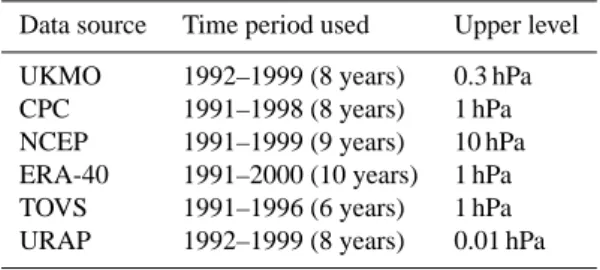
Table 1. Climatological data sets used for model validation.
Data source Time period used Upper level UKMO 1992–1999 (8 years) 0.3 hPa CPC 1991–1998 (8 years) 1 hPa NCEP 1991–1999 (9 years) 10 hPa ERA-40 1991–2000 (10 years) 1 hPa TOVS 1991–1996 (6 years) 1 hPa URAP 1992–1999 (8 years) 0.01 hPa
2.3 GCM-CTM interface
For the coupling with MA-ECHAM4, MEZON has been im-proved to take into account the latest revisions of the chem-ical reaction constants. Several photolytic and gas-phase re-actions that are potentially important for mesospheric chem-istry have been added to the model. The new scheme for photolysis rate calculations spans the spectral region 120– 750 nm divided into 73 spectral intervals and now specifi-cally includes the Lyman-α line and the Schumann-Runge continuum. We have tested its performance using a 1-D chemistry-climate model (Rozanov et al., 2002b). The GCM and CTM components of SOCOL are coupled via the three-dimensional fields of wind, temperature, ozone and water va-por. The GCM provides the horizontal and vertical winds, temperature and tropospheric humidity for the CTM, which returns 3-D fields of the ozone and water vapor mixing ra-tios back to the GCM in order to calculate radiation fluxes and heating rates. The water cycle in the troposphere and lower stratosphere is treated in the GCM part of the model, while the water vapor chemistry and transport in the strato-sphere and mesostrato-sphere is treated in chemistry-transport part of the model. The unique water vapor field is transferred from GCM to CTM and back at every step.
2.4 Community model
To make SOCOL available for a wide scientific community we ported the entire CCM on desktop personal computers (PCs). A 10-year long simulation takes about 40 days of wall-clock time on a PC with a processor running at 2.5 GHz, which allows the performance of multiyear integrations. The simultaneous use of several PCs allows the performance of ensemble calculations with ease. Reasonable model perfor-mance and availability of personal desktop computers makes SOCOL available for application by scientific groups around the world without access to large super-computer facilities, opening wide perspectives for model exploitation and im-provement. The technical information is given at the end of the paper.
2.5 Model set-up
As a first step toward the validation of SOCOL we have car-ried out a 40-year long control run for present day condi-tions. For this run we used sea surface temperature and sea ice (SST/SI) distributions prescribed from AMIP II monthly mean distributions, which are averages from 1979 to 1996 (Gleckler, 1996). The lower boundary conditions for the source gases have been prescribed following Rozanov et al. (1999) and are representative for conditions of 1995. We use prescribed mixing ratios in the planetary boundary layer for the source gases and prescribed fluxes of CO and NOx
from the surface, airplanes and lightning, similar to Rozanov et al. (1999). The mixing ratio of CO2 is set to 356 ppmv
everywhere. The initial distributions of the meteorological quantities and gas mixing ratios have been adopted from MA-ECHAM4 and from an 8-year long Stratospheric CTM run (Rozanov et al., 1999). Later on in this paper we will analyze the 40-year mean of the simulated quantities.
3 Description of the data used for validation
To validate the large-scale atmospheric behavior of the SO-COL model and to specify the significance of the model er-rors we use data sets for the middle atmosphere which are the results of the efforts of different meteorological institu-tions around the world: the European Center for Medium Range Weather Forecast (ECMWF), United Kingdom Me-teorological Office (UKMO), National Center of Environ-mental Predictions (NCEP) and Climate Prediction Center (CPC) reanalysis projects. We have also used monthly mean data obtained from the TOVS instrument. All data sets have been downloaded from the SPARC Data Center (http://www. sparc.sunysb.edu). Detailed descriptions of the data sets used have been presented in the SPARC inter-comparison project of the middle atmosphere (SPARC, 2002). Some charac-teristic parameters of the applied data sets are summarized in Table 1. According to the SPARC comparison report (SPARC, 2002) UKMO, CPC and NCEP are warm biased in the tropical tropopause area by 2–3 K, while UKMO has a warm bias in the upper stratosphere up to 5 K. To estimate the significance of the deviation of the simulated climatology from the observed climatology we have combined all data sets listed in Table 1 (except URAP data) in one data set. In doing this we obtained 41 consecutive years of observational data for the validation (only 32 include data above 10 hPa). From this extended data set we have calculated a monthly mean climatology of the zonal wind and temperature, as well as the standard deviation of these quantities, which includes the interannual variability as well as variability due to differ-ences between data sets. To validate the model winds in the mesosphere we used URAP (http://code916.gsfc.nasa.gov) zonal mean zonal wind, which is a combination of UKMO winds in the stratosphere and the High Resolution Doppler
Fig. 1. Meridional cross-section of the zonal mean zonal wind (ms−1)for January (left panel) and July (right panel): (a, b) simulated, (c, d) observed. Observed values are from URAP database.
Imager (HRDI) winds in the mesosphere (Swinbank and Or-tland, 2003).
Total ozone data have been taken from merged TOMS/SBUV data set (http://code916.gsfc.nasa.gov/Data services/merged/mod data.public.html) and averaged over 10 years (1991–2000). For the comparison of ozone (O3),
water vapor (H2O), methane (CH4)and HCl in the
strato-sphere we used the URAP data set (http://code916.gsfc.nasa. gov) that provides a comprehensive description of the refer-ence stratosphere from the data recorded by several instru-ments onboard of UARS. Because we used only one data set for every considered species the standard deviation in this case is defined only by interannual variability. For all consid-ered quantities the differences of the simulated and observed fields are considered as significant if they exceed the sum of the standard deviations of the simulated and observed fields. To analyze the response of the atmosphere to the strength of the polar vortex we use the same 40-year long simulation of the present day atmosphere. We divided the simulated data into two groups according to the phase of Arctic Oscil-lation during the boreal winter season defined from the prin-cipal component of the first EOF of the geopotential height field at 70 hPa and contrasted the difference between these two groups against observational data processed in an iden-tical way. The statisiden-tical significance of this difference is estimated using the well known Student’s t-test. The obser-vations we used are NMC data (for 1978–1998) and SAGE I/II ozone density (for 1979–2001) compiled by W. Randel et al. (www.acd.ucar.edu/∼randel).
4 Results
4.1 Monthly mean zonal mean zonal wind and temperature 4.1.1 Temperature and wind fields
Monthly means of zonally averaged zonal winds for January and July are presented in Fig. 1 in comparison with the 8-year means of the same quantities acquired from the URAP data sets. The model reproduces all the main climatologi-cal features of the observed zonal wind distribution qualita-tively, and with a few exceptions even quantitatively. The separation of the stratospheric and tropospheric westerly jets is well simulated by SOCOL. The tropospheric subtropical jets, their shape and location are in good agreement as is the polar night jet (PNJ) core, in the middle and upper strato-sphere. However, for January in the Northern Hemisphere the intensity of the tropospheric subtropical jet is overesti-mated by about 10 ms−1. The PNJ’s intensity is underesti-mated by the same amount, and its maximum is located at higher altitudes than in the URAP data. SOCOL captures the observed equatorward tilt of the stratospheric westerly core. The most noticeable disagreement occurs in the lower mesosphere, where the simulated easterly winds do not pene-trate to the high-latitude area over the summer hemisphere. It should be noted that the model does not reproduce the QBO in the equatorial atmosphere, which can affect the simulated climatology of the temperature, winds and chemical species (Giorgetta et al., 2004).
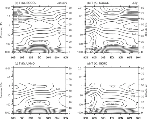
Fig. 2. Same as Fig. 1 but for the zonal mean temperature (K). Observed values are from UKMO reanalysis.
Fig. 3. Zonal mean zonal wind for January and July from the observation data composite (a, b) (contours in steps of 10 ms−1)and difference (contours in steps of 5 ms−1)between simulated and observed data (c, d). Shading marks “hotspots”, the area where the deviations are significant.
Figure 2 presents a comparison of latitude-pressure cross-sections of simulated and UKMO zonal mean temperatures for January and July. The evaluation of the temperature dis-tribution reveals that in the lower stratosphere the general
agreement of the location and magnitude of the simulated ex-tremes is rather good. SOCOL reproduces the main observed features of zonal mean temperature distribution well: warm troposphere, cold tropical tropopause without apparent bias,
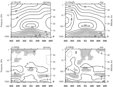
Fig. 4. Same as for Fig. 3, but for temperature (contours in steps of 10 K and 5 K accordingly).
Fig. 5. Seasonal variation of the simulated temperature and zonal wind deviations from the observation data at 1, 10 and 70 hPa. Shading
90S 60S 30S EQ 30N 60N 90N 100 10 1 0.1 Pressure, hPa 0.2 0.6 1.0 1.4
(a) CH4 (ppmv), SOCOL Jan
90S 60S 30S EQ 30N 60N 90N 20 30 40 50 60 90S 60S 30S EQ 30N 60N 90N 100 10 1 0.1 Pressure,hPa 0.2 0.2 0.2 0.6 1.0 1.4 (b) CH4 (ppmv), URAP 90S 60S 30S EQ 30N 60N 90N 20 30 40 50 60 90S 60S 30S EQ 30N 60N 90N 100 10 1 0.1 Pressure, hPa -20 0 0 0 20 (c) ∆CH4 (%) 90S 60S 30S EQ 30N 60N 90N 20 30 40 50 60 90S 60S 30S EQ 30N 60N 90N 100 10 1 0.1 Pressure, hPa -50 -50 -50 50 (d)∆CH4 (ppbv) 90S 60S 30S EQ 30N 60N 90N 20 30 40 50 60 90S 60S 30S EQ 30N 60N 90N 100 10 1 0.1 0.2 0.6 1.0 1.4
(e) CH4 (ppmv), SOCOL Jul
90S 60S 30S EQ 30N 60N 90N 20 30 40 50 60 Altitude, km 90S 60S 30S EQ 30N 60N 90N 100 10 1 0.1 0.2 0.2 0.6 1.0 1.4 (f) CH4 (ppmv), URAP 90S 60S 30S EQ 30N 60N 90N 20 30 40 50 60 Altitude, km 90S 60S 30S EQ 30N 60N 90N 100 10 1 0.1 -20 0 0 0 20 20 (g) ∆CH4 (%) 90S 60S 30S EQ 30N 60N 90N 20 30 40 50 60 Altitude, km 90S 60S 30S EQ 30N 60N 90N 100 10 1 0.1 (h)∆CH4 (ppbv) -100 -50 -50 -50 0 0 0 50 90S 60S 30S EQ 30N 60N 90N 20 30 40 50 60 Altitude, km
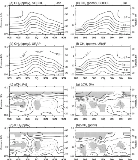
Fig. 6. Latitude-pressure cross-section of the CH4(ppmv) for January (left panel) and July (right panel): simulated (a, b), observed (b, e),
and their differences in steps of ±1% (c, d) and of ±50 ppbv (d, h). Observed values are from URAP data set. Shading marks “hotspots”, the area where the deviations are significant.
cold winter middle stratosphere, warm summer stratopause, and the polar temperature minimum associated with the for-mation of the polar vortices.
4.1.2 Model/observation difference fields
A simple visual comparison of temperature and zonal wind fields has often been used to validate CCMs (e.g., Takigawa et al., 1999; Hein et al., 2001). From this kind of compar-ison one can only conclude how well a model reproduces the main observed features of the zonal mean temperature and zonal mean zonal wind structures in general. However, differences between simulated and observed fields do exist and it is very helpful to use a more quantitative analysis of model deviations from observations as it has been presented by Rozanov et al. (2001) and Jonsson et al. (2002). Due to noticeable discrepancies among the available reanalysis data (e.g., SPARC, 2002) it is difficult to judge the model per-formance precisely and to give recommendations on how a
model could be improved. To estimate the significance of the model deficiencies we use a monthly mean observed cli-matology of the zonal wind (see Figs. 3a, b) and temperature (see Figs. 4a, b) and the standard deviation of these quantities described in Sect. 3. From the results of the 40-year long SO-COL integration we have also calculated the climatology of the zonal wind (see Figs. 1a, b) and temperature (see Figs. 2a, b) and their standard deviations. Using these data sets we have calculated the difference between the simulated and ob-served climatology and estimated the significance of these deviations. The difference between the simulated and ob-served fields is defined as significant if it exceeds the sum of the standard deviations of the simulated and observed fields. Figures 3c, d and 4c, d show ensemble mean monthly mean deviations of the model from the observational data in January and July for zonal means of zonal wind and temper-ature respectively. The gray spots mark the area where the model deviations from the observational data are significant. In the zonal wind field these spots appear in the region of the
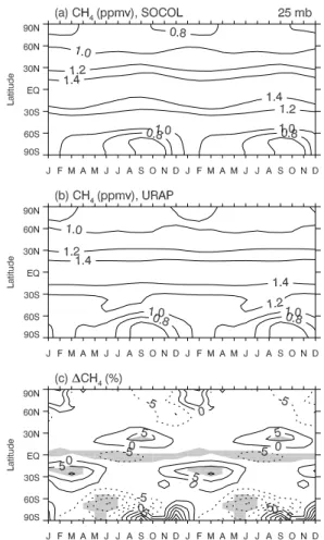
Fig. 7. Seasonal variations of the methane mixing ratio at 25 hPa: (a) simulated, (b) observed, and (c) their difference in percent.
Observed values are from the URAP data set. Shading marks “hotspots”, the area where the deviations are significant.
extra tropical jets implying that SOCOL has a tendency to reproduce stronger (up to 5–10 m/s) jets in the upper tropo-sphere. The marginally significant westerly bias (5–10 m/s) around 10 hPa and the weak easterly bias (∼5 m/s) around 40 hPa could be the result of the lack of QBO in the model and slight westerly QBO bias in the observation data. All other deviations appear to be insignificant. In the temperature field (Figs. 4c, d) the model substantially deviates from the observational data near the extra-tropical tropopause. The simulated temperature has a significant warm bias in the upper stratosphere in the tropics and in the summer hemi-sphere over high and middle latitudes. At the high lat-itude tropopause the discrepancies between simulated and observed data reach about –6 K during winter and in the summer the deviation is up to –10 K. In the tropical lower stratosphere the simulated temperature has a cold bias of up to –6 K and a weak positive bias just above this layer, which resembles the temperature anomalies due to the QBO (Giorgetta et al., 2004). The deviations are mostly negative, showing that the model is cold biased relative to the data.
the simulated temperature deviations from the observations are insignificant, except a small (–3 K) negative bias at 30◦S and 30◦N. The simulated zonal wind at 10 hPa deviates in the tropics during boreal summer, however, the deviations do not exceed 10 ms−1and are only marginally significant. In
the lower stratosphere the model has a cold bias at the equa-tor, of up to 9 K, and a warm bias of up to 3 K in the extra tropical area. The simulated zonal wind at 70 hPa has an easterly bias in the tropical area and a westerly bias over the middle latitudes with a magnitude of 5 ms−1, however these biases are only marginally significant.
4.1.3 Summary
From the analysis of the zonal mean and seasonal variations of the zonal wind and temperature we conclude that dur-ing warm seasons our model does not have enough heatdur-ing in the upper stratosphere at high latitudes and at the equa-tor. This might be connected to the problem in the radiation code of MA-ECHAM4, which describes the absorption of solar UV radiation by ozone and oxygen with a rather sim-plified scheme. We will return to this problem in Sect. 5. The temperature differences are most pronounced near the tropopause. These model deficiencies over high latitudes can be explained by the rough vertical model resolution in the up-per troposphere-lower stratosphere (Roeckner et al., 2004). Some part of the cold bias in the tropical lower stratosphere can be explained by the absence of the QBO in the model (Giorgetta et al., 2004).
5 Chemical aspects of the validation
5.1 Methane
Altitude dependence. Methane is the most abundant
hydro-carbon in the atmosphere and is useful as a tracer of atmo-spheric circulation because of its long photochemical life-time (∼8–9 years in the global atmosphere). Hence, the methane distribution is determined mainly by features of the circulation. Figure 6 shows the meridional cross section of the CH4mixing ratio climatology simulated by SOCOL and
observed by UARS together with their difference. The over-all modeled zonal mean distribution (CH4 decreases with
90S 60S 30S EQ 30N 60N 90N 100 10 1 0.1 Pressure, hPa 4.0 5.0 6.0 7.0
(a) H2O (ppmv), SOCOL Jan
90S 60S 30S EQ 30N 60N 90N 20 30 40 50 60 90S 60S 30S EQ 30N 60N 90N 100 10 1 0.1 Pressure,hPa 4.0 5.0 6.0 (b) H2O (ppmv), URAP 90S 60S 30S EQ 30N 60N 90N 20 30 40 50 60 90S 60S 30S EQ 30N 60N 90N 100 10 1 0.1 Pressure, hPa 0 0 10 10 10 20 20 20 (c) ∆H2O (%) 90S 60S 30S EQ 30N 60N 90N 20 30 40 50 60 90S 60S 30S EQ 30N 60N 90N 100 10 1 0.1 Pressure, hPa 0.5 0.5 1.5 (d)∆H2O (ppmv) 90S 60S 30S EQ 30N 60N 90N 20 30 40 50 60 90S 60S 30S EQ 30N 60N 90N 100 10 1 0.1 5.0 5.0 6.0 7.0
(e) H2O (ppmv), SOCOL Jul
90S 60S 30S EQ 30N 60N 90N 20 30 40 50 60 Altitude, km 90S 60S 30S EQ 30N 60N 90N 100 10 1 0.1 4.0 4.0 5.0 6.0 (f) H2O (ppmv), URAP 90S 60S 30S EQ 30N 60N 90N 20 30 40 50 60 Altitude, km 90S 60S 30S EQ 30N 60N 90N 100 10 1 0.1 10 10 10 20 20 20 30 (g) ∆H2O (%) 90S 60S 30S EQ 30N 60N 90N 20 30 40 50 60 Altitude, km 90S 60S 30S EQ 30N 60N 90N 100 10 1 0.1 (h)∆H2O (ppmv) 0.5 1.0 1.0 1.5 1.5 90S 60S 30S EQ 30N 60N 90N 20 30 40 50 60 Altitude, km
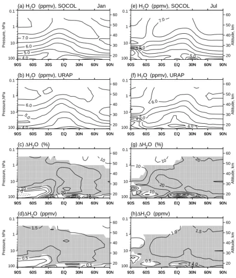
Fig. 8. Same as for Fig. 6, but for water vapor.
of transport by the Brewer-Dobson circulation, the tropical maxima of CH4 concentration is shifted to the North
dur-ing boreal summer and to the South durdur-ing boreal winter. The subtropical transport barriers are also reasonably sim-ulated. The model significantly overestimates the methane mixing ratio in the mesosphere, which could be connected to the underestimation of chemical methane destruction by the hydroxyl or methane photolysis in Lyman-α line. Signif-icant deviations of the simulated methane mixing ratio from the observations also take place in the middle stratosphere implying less intensive methane transport by the meridional circulation. The underestimation of the circulation intensity can be partially explained by the absence of the QBO in the model (Girogetta et al., 2004). The model reasonably repro-duces the downward motion over the northern high latitudes in January, however in the Southern Hemisphere the polar vortex is too strong, leading to an underestimation of the CH4
mixing ratio at 10 hPa by more then 20 % (∼100 ppbv).
Seasonal cycle. Latitude-time variations in the observed and
simulated zonal average mixing ratio of CH4 at 25 hPa are
shown in Fig. 7. The model reproduces the seasonal
varia-tion over the middle and high latitudes, which is similar to the HALOE data with a relative minimum over the high lati-tudes during December-February for the NH and September– November for the SH, while in the tropical area the simu-lated methane mixing ratio has a seasonal cycle, in contrast to the UARS data, which shows no apparent seasonal cycle. At 25 hPa, significant differences between simulated and ob-served data in the tropics are about ±5% and in the southern high latitudes the difference reaches –15% in May–June be-cause of the downward transport of the air with low methane mixing ratio from the upper stratosphere starts earlier in the model than in the observations.
5.1.1 Water vapor
Altitude dependence. Water vapor is an important tracer
in the upper troposphere and lower stratosphere. In both re-gions H2O is a source of HOxradicals, which are involved
in photosmog reactions producing ozone in the upper tropo-sphere and in catalytic ozone destruction cycles in the strato-sphere. Figure 8 presents meridional cross-sections of water
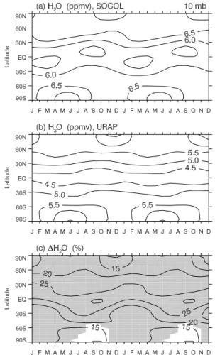
Fig. 9. Same as for Fig. 7 but for water vapor at 10 hPa.
vapor mixing ratios. The shape of the zonal-mean H2O
dis-tribution is well reproduced by SOCOL. However, the model overestimates mixing ratio of H2O compared to URAP data
in the stratosphere by 0.5–1.0 ppmv (or 10–20%), which is within the range of accuracy of HALOE measurements (Har-ries et al., 1996). There are two sources of H2O in the
strato-sphere: CH4oxidation in the stratosphere and upward
trans-port of H2O from the troposphere. The latter depends in
turn on the intensity of the upward branch of the Brewer-Dobson circulation, which determines vertical transport and on the H2O mixing ratio at the entry level. The H2O
mix-ing ratio in the stratosphere is defined by chemical produc-tion from the methane oxidaproduc-tion cycle and by transport pro-cesses. Chemical destruction by reaction with exited oxygen plays a less important role. Transport processes tend to make stratospheric H2O closer to the H2O mixing ratio at the
en-try level, which is located in the tropical UTLS. Therefore, stronger circulation would usually lead to a decrease of the stratospheric H2O. This means that in general, the
overes-timation problems of stratospheric H2O can be caused by:
(i) overestimated chemical production, (ii) underestimated intensity of the meridional circulation; and (iii) overestima-tion of the H2O mixing ratio at the entry level. Figure 6
J F M A M J J A S O N D J F M A M J J A S O N D 15 -0.30 -0.050.00 0.00 J F M A M J J A S O N D J F M A M J J A S O N D 15 20 25 30 35 40 45 50 55 60 Height,km (b) Anomaly H2 O (ppmv), URAP -0.50 -0.50 -0.30 -0.30 -0.10 -0.10 -0.10 -0.10 -0.10 -0.10 -0.10 -0.10 0.00 0.00 0.00 0.00 0.00 0.00 0.00 0.00 0.00 0.20 0.20 0.20 0.20 0.40 0.40
Fig. 10. Altitude-time evolution of water vapor mixing ratio over
the equator, derived from (a) SOCOL simulation and (b) HALOE observation. Twelve months of climatological data are repeated twice. The negative (positive) contours are labeled in steps of – 0.05 (0.1) ppmv. 0 2 4 6 8 10 12 lag (month) 0.0 0.2 0.4 0.6 0.8 Rcorr
Fig. 11. Lagged correlation coefficients of deseasonalised H2O mixing ratio anomalies in the equatorial stratosphere at 16 km with the same quantity at 19.4 (solid line), 22.7 (dotted line), 25.9 (dashed line), 29.1 (dot-dashed line) and 32.3 (dot-dot-dashed line) km levels.
60S 30S EQ 30N 60N 100 10 1 0.1 Pressure, hPa 1.0 2.0 3.0
(a) HCl (ppbv), SOCOL Jan
60S 30S EQ 30N 60N 20 30 40 50 60 60S 30S EQ 30N 60N 100 10 1 0.1 Pressure,hPa 1.0 2.0 3.0 (b) HCl (ppbv), URAP 60S 30S EQ 30N 60N 20 30 40 50 60 60S 30S EQ 30N 60N 100 10 1 0.1 Pressure, hPa -20 10 10 30 (c) ∆HCl (%) 60S 30S EQ 30N 60N 20 30 40 50 60 60S 30S EQ 30N 60N 100 10 1 0.1 Pressure, hPa -0.2 0.2 0.6 0.6 0.6 (d)∆HCl (ppbv) 60S 30S EQ 30N 60N 20 30 40 50 60 60S 30S EQ 30N 60N 100 10 1 0.1 1.0 2.0 3.0
(e) HCl (ppbv), SOCOL Jul
60S 30S EQ 30N 60N 20 30 40 50 60 Altitude, km 60S 30S EQ 30N 60N 100 10 1 0.1 1.0 2.0 3.0 (f) HCl (ppbv), URAP 60S 30S EQ 30N 60N 20 30 40 50 60 Altitude, km 60S 30S EQ 30N 60N 100 10 1 0.1 -20 10 10 30 (g) ∆HCl (%) 60S 30S EQ 30N 60N 20 30 40 50 60 Altitude, km 60S 30S EQ 30N 60N 100 10 1 0.1 (h)∆HCl (ppbv) 0.0 0.0 0.2 0.4 0.4 0.4 0.6 0.6 60S 30S EQ 30N 60N 20 30 40 50 60 Altitude, km
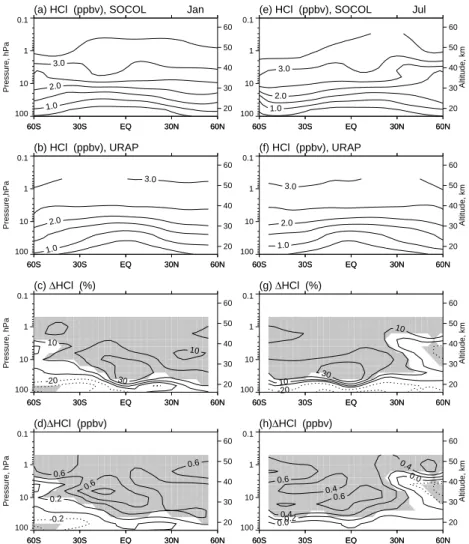
Fig. 12. Same as for Fig. 6 but for HCl (contour lines in steps of 0.5 ppbv). The difference in (c ,g) is shown in steps of ±10% and in (d, h)
is shown in steps of ±0.2 ppbv.
shows a small (∼0.1 ppmv) deviation of CH4mixing ratios
in the middle stratosphere from the URAP data, which could explain only ∼0.2 ppmv of the deviation of H2O mixing
ra-tios. However, it is clear from Fig. 8 that the simulated H2O
mixing ratio are overestimated by at least 1 ppmv, which im-plies that only the intensity of the meridional circulation or H2O mixing ratio at the entry level could be responsible. A
slight underestimation of the simulated methane in compari-son with URAP data implies that the intensity of the merid-ional transport in our model is underestimated, therefore the overestimation of stratospheric H2O could be connected to
the slower meridional circulation or an overestimated H2O
mixing ratio at the entry level. The later is more plausible explanation because the analysis of Figs. 8d ,j shows that the deviation of the H2O mixing ratio in the stratosphere from
URAP data is close to the deviation at the entry level.
Seasonal cycle. The seasonal variation of simulated H2O
mixing ratios at 10 hPa is compared with URAP data in Fig. 9. The model and URAP data do not show a sufficiently
strong annual cycle in the tropical middle stratosphere. Over the high latitudes both model and observations reveal ele-vated H2O mixing ratios during wintertime, associated with
aged air chemically depleted with respect to CH4,
descend-ing into the polar vortices.
Figure 10 presents a comparison of the simulated and URAP-derived data set of the altitude-time anomaly in the H2O mixing ratio (deviation from annual mean) over the
equator. The model reproduces the vertical propagation of the dry (negative) and wet (positive) anomalies induced by the water vapor changes in the lower stratosphere, i.e. the water vapor “tape recorder” described by Mote et al. (1998). However, the model upward transport is up to twice as fast as observed. In order to quantitatively estimate the inten-sity of the upward water vapor transport we have calculated lagged correlations between deseasonalized H2O mixing
ratio anomalies at 16 km altitude and at different altitudes in the equatorial stratosphere. The correlation coefficients are plotted in Fig. 11 for the 19.4, 22.7, 25.9, 29.1 and 32.3 km
90S 60S 30S EQ 30N 60N 90N 100 10 Pressure,hPa 2 4 6 8 90S 60S 30S EQ 30N 60N 90N 20 30 40 90S 60S 30S EQ 30N 60N 90N 100 10 1 0.1 Pressure, hPa -20 0 0 0 20 40 40 (c) ∆O3 (%) 90S 60S 30S EQ 30N 60N 90N 20 30 40 50 60 90S 60S 30S EQ 30N 60N 90N 100 10 1 0.1 Pressure, hPa 0.0 0.0 (d)∆O3 (ppmv) 90S 60S 30S EQ 30N 60N 90N 20 30 40 50 60 90S 60S 30S EQ 30N 60N 90N 100 10 2 4 6 8 90S 60S 30S EQ 30N 60N 90N 20 30 40 Altitude, km 90S 60S 30S EQ 30N 60N 90N 100 10 1 0.1 -20 0 0 0 0 0 20 40 (g) ∆O3 (%) 90S 60S 30S EQ 30N 60N 90N 20 30 40 50 60 Altitude, km 90S 60S 30S EQ 30N 60N 90N 100 10 1 0.1 (j)∆O3 (ppmv) -1.0 -0.5 0.0 0.0 0.5 90S 60S 30S EQ 30N 60N 90N 20 30 40 50 60 Altitude, km
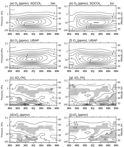
Fig. 13. Same as for Fig. 6 but for O3(contour lines in steps of 1 ppmv). ). The difference in (c ,g) is shown in steps of ±10% and in (d, h)
is shown in steps of ±0.5 ppbv.
levels. The time when the maximum correlation is reached and the distance between levels allow the estimation of the vertical velocities in the equatorial lower stratosphere. For the plotted data the mean vertical velocity between 16 and 32.3 km is equal to ∼0.6 mm/s, which exceeds the value obtained from the observed H2O distribution by about 50–
90%. The vertical velocity is larger in the lower stratosphere (around 1 mm/s), while between 29.1 and 32.3 km its mag-nitude is about 0.25 mm/s. Similar distributions of the ver-tical velocities have been reported by Steil et al. (2003). It is still not clear which part of the model is responsible for these discrepancies between the simulated and observed “tape recorder” features. In the upper stratosphere the model quantitatively matches the observed semi-annual oscillation with positive anomalies during the boreal summer (Fig. 10).
5.1.2 HCl
HCl is a reservoir species for the chlorine group. Its mixing ratio in the upper stratosphere and mesosphere characterizes the level of the total reactive chlorine available for the istry. HCl plays an important role in the polar ozone chem-istry, providing a source for active chlorine radicals through the heterogeneous chlorine activation process. The simu-lated distribution of HCl for January and July is presented in Fig. 12 in comparison with URAP data. The simulated HCl mixing ratio mimics some of the observed features. The HCl mixing ratio increases with altitude from ∼0.5 ppbv in the lower stratosphere up to 3.5 ppbv in the mesosphere. The model also captures the observed decrease of the HCl mixing ratio with latitude in the lower stratosphere and an uniform latitudinal distribution in the middle stratosphere. However, the observed latitudinal gradient is much steeper in the lower stratosphere than in the simulations. The overall agreement is within ∼20%, but the error exceeds 30% in the tropical lower
Fig. 14. Seasonal variation of the total ozone: (a) simulated, (b)
observed, and (c) their difference in percents. The observed values are from TOMS/SBUV merged data set. Shading marks “hotspots”, the area where the deviations are significant.
stratosphere where the HCl mixing ratio is much lower. The simulated HCl mixing ratio is systematically overestimated by the model, which can be related in part to the underesti-mated intensity of the meridional circulation and in part to the model run set-up. Here we analyze the results of the 40-year model run performed with the mixing ratio of the source gases typical for the year 1995. Because of the 5–6 year time lag between stratospheric chlorine and the total chlorine in the near surface air, the stratospheric chlorine in our steady-state run are more representative of the late 90’s . On the other hand, the URAP climatology of HCl in more represen-tative of the earlier 90’s, when the HCl mixing ratio should be to some extent lower than during the late 90’s.
5.1.3 Ozone
Altitude dependence. Figure 13 illustrates meridional cross
sections of zonal mean monthly mean O3mixing ratios,
sim-ulated by SOCOL and observed by UARS together with their difference. The distribution of the simulated ozone is in relatively good agreement with the observations through-out the stratosphere where the model errors remain basically within ±10%. The simulated maximum of the zonal mean (∼9 ppmv) appears at the equator, at around 10 hPa, which is consistent with the observations. The so-called “banana”
shape of the ozone distribution is also well captured by the model with high ozone regions extending to the upper polar stratosphere. The model significantly underestimates ozone over the southern high latitudes in the upper stratosphere dur-ing the austral winter season. The cause of the ozone un-derestimation could be in part related to (or identical to) the causes as for the underestimation of methane and the overes-timation of water vapor in the same region: this could stem from a too strong isolation of the southern polar vortex and a too strong downward transport in the model. The fact that methane is longer-lived than ozone in these regions could be the reason for the methane discrepancy appearing only at lower altitudes. An underestimation of ozone in the up-per stratosphere could in part explained by the overall over-estimation of the reactive chlorine mentioned in Sect. 4.2.3, which leads to more intensive ozone destruction. The devia-tion of simulated ozone from the observadevia-tion cannot explain the significant cold temperature bias near the stratopause (shown in Fig. 4). From our 1-D model (Rozanov et al., 2002b) we estimate that even –10% ozone deficit could pro-vide a cooling of only about 1.5 K. A small positive bias in the tropical lower stratosphere around 40 hPa and a negative bias at 10 hPa can be explained by the absence of the QBO in the model (Giorgetta et al., 2004).
Seasonal cycle. The comparison of the seasonal variation
of the simulated total ozone column (TOC) with the obser-vations is presented in Fig. 14. SOCOL reproduces a sea-sonal maximum in the NH and a maximum and minimum in the SH with reasonable accuracy. The overall agreement be-tween the model and the observation data composite is within
±5% in the tropics, ±10% in the northern middle and high latitudes, and within ±10–20% in the southern middle and high latitudes. Significant deviations of the simulated total ozone from the TOMS climatology occur mostly from Jan-uary to May and consists of an underestimation of the to-tal ozone over the northern high latitudes and overestimation over the middle southern latitudes. This redistribution of the total ozone can be also explained by the above-mentioned slower-than-observed meridional circulation in the model. A similar pattern of the total ozone deviation appears again dur-ing austral winter and sprdur-ing, however the total ozone de-viations over the southern high latitudes are not significant, implying a good performance of the model in the area of the ozone “hole”. Figure 15 illustrates the total ozone simu-lated by SOCOL in March over the NH and in October over the SH in comparison with corresponding satellite observa-tions. The position and magnitude of the ozone “hole” is very well reproduced by SOCOL, confirming that the amount of PSCs during the spring season and chemical ozone destruc-tion are reasonably well captured by the chemical routine of the model. The position of the total ozone maximum in the Australian sector is also well captured by SOCOL. The mag-nitude of the maximum is slightly underestimated, but this deviation is not significant. Some CCMs (see Austin et al., 2003, their Fig. 2) substantially overestimate the magnitude
c) March, observation 275 275 300 300 325 350375 e) March, Diff (%) -10 -5 0 0 d) October, observation 200 275 325 375 f) October, Diff (%) -10 0 0 0 0 0
Fig. 15. Geographical distribution of the simulated (a, b) and observed (c, d) total ozone for March over the Northern Hemisphere and
Octo-ber over the Southern Hemisphere in Dobson Units (DU) and their difference (e, f) in percents. The observed values are from TOMS/SBUV merged data set. Shading marks “hotspots”, the area where the deviations are significant.
of the total ozone maxima over the middle latitudes in the Australian sector. This could imply that the relevant wave forcing and subsequently meridional transport in these mod-els are too strong, but SOCOL seems not to suffer from this problem. In March over the Northern Hemisphere, however, the underestimation of the simulated total ozone is more pro-nounced (up to 15%) and significant over Pacific and North American sectors. As was mentioned before it could be a result of a weak meridional circulation in the model.
We have compared the pattern correlation and absolute de-viation (not shown) of area weighted total ozone simulated
by SOCOL and simulated by CCMs that participated in the model intercomparison presented by (Austin et al., 2003). The comparison shows that among the other models SOCOL has the smallest absolute deviation from the observations in the SH, which is ∼5% and very high pattern correlation (more than 0.95) over both hemispheres. Over the Northern Hemisphere SOCOL underestimates the total ozone maxi-mum in March by about 50 DU, but nevertheless has one of the smallest absolute deviations (∼5%) of total area weighted ozone over the NH from the observational data among the models compared by Austin et al. (2003).
Fig. 16. Observed and simulated differences between positive and
negative AO phase in the zonal mean geopotential heights (m). Shading marks the area where the difference is statistically signifi-cant at 90% confidence level.
Fig. 17. Observed and simulated differences between positive and
negative AO phase in the zonal mean zonal wind (ms−1). Shading marks the area where the difference is statistically significant at 90% confidence level.
5.2 Sensitivity of ozone and temperature to the strength of the Arctic winter vortex
As was mentioned in Sect. 3 we divided the simulated and observed data into two groups according to the phase of Arctic Oscillation during the boreal winter season to
Fig. 18. Observed and simulated differences between positive and
negative AO phase in the zonal mean temperature (K). Shading marks the area where the difference is statistically significant at 90% confidence level.
Fig. 19. Observed and simulated differences between positive and
negative AO phase in the zonal mean ozone mixing ratio (%).Shad-ing marks the area where the difference is statistically significant at 90% confidence level.
analyze the response of the atmosphere to the strength of the polar vortex. Figures 16–19 illustrate the differences between these two composites in zonal mean geopotential height, zonal wind, temperature and ozone mixing ratio av-eraged over the boreal winter season (December–January– February). Figure 16 shows that the simulated and observed
sphere. In the tropics, the model matches the observed warm-ing in the lower stratosphere, although the magnitude of the simulated warming is about 2 times smaller. The simu-lated and observed temperature changes in the upper tropi-cal stratosphere are not statistitropi-cally significant. The ozone response is shown in Fig. 19. The simulated and observed changes are in qualitative agreement only in the lower trop-ical stratosphere, where the model simulates a statisttrop-ically significant increase the ozone mixing ratio. This theoreti-cally expected feature is also visible in the observation data, however it does not appear to be statistically significant. In the model the warming in the tropical stratosphere and sub-sequent decrease of the equator-pole temperature gradient in the Southern Hemisphere leads to the westerly acceleration of the zonal wind in the stratosphere over middle latitudes, formation of the dipole-like structure and negative anomalies in the geopotential heights over the high latitudes. However, none of these features can be seen in the observation data, therefore it is hard to say how real they are.
6 Conclusions
In this paper we presented a description of a new modeling tool, the CCM SOCOL, together with the validation of the simulated present-day climatology against a variety of ob-servational data. We also present an example of processes-oriented validation. While the model performance is quite satisfactory based on an overall inspection of simulated fields and on a proper statistical analysis, we have identified a num-ber of weaknesses that need to be addressed for the future improvement of the model. In particular, the analysis of the simulated zonal wind and temperature deviations shows that for an improvement it will be necessary to pay special atten-tion to the tropopause region at high latitudes as well as to the description of the processes in the upper stratosphere and mesosphere, where significant cold biases have been found in the model during boreal summer.
The model’s too cold upper stratosphere is most likely re-lated to the radiation code of MA-ECHAM4 (see Sect. 4), which does not take into account the absorption of solar ir-radiance for wavelengths shorter than 250 nm. To illustrate the importance of this spectral region we have applied a 1-D radiative convective model (RCM) described by Rozanov
Fig. 20. Temperature difference due to absorption of the solar
ir-radiance in the 120–250 nm spectral interval calculated with 1-D RCM for three cases: Tropical atmosphere model, SZA=45◦, du-ration of the day=12 h (solid line); Middle latitude summer atmo-sphere model, SZA=60◦, duration of the day=14.4 h (dashed line); Subarctic summer atmosphere model, SZA=70◦, duration of the day=24 h (dash-dotted line).
et al. (2002b) and calculated the temperature profiles with and without absorption of the solar irradiance in the spec-tral region 120–250 nm. Temperature differences due to ab-sorption of the solar irradiance in the 120–250 nm spectral interval have been calculated with the 1-D RCM for three cases: (1) a tropical atmosphere model, with Solar Zenith Angle (SZA)=45◦, duration of the day (DoD)=12 h; (2) a
middle latitude summer atmosphere model, with SZA=60◦,
DoD=14.4 h; (3) a subarctic summer atmosphere model, with SZA=70◦, DoD=24 h. The results are depicted in Fig. 20, suggesting that near the stratopause the contribution of the 120–250 nm spectral region could reach up to 9 K. Therefore we hypothesize that the missing source of heat would sub-stantially improve temperature and zonal wind distributions in the summer extra-tropical upper stratosphere and meso-sphere also in the 3-D model.
The simulated descent of air is too strong in the polar stratosphere, leading to a significant underestimation of CH4
and O3mixing ratios in this area. An analysis of the water
vapor zonal mean and seasonal distributions reveals an over-estimation of stratospheric H2O, which is probably related to
the transport of H2O from the troposphere. The analysis of
the total ozone and some other quantities suggests that the simulated meridional circulation is too weak. For the fur-ther improvement of the model the parameterization of the unresolved wave forcing should be reconsidered to provide stronger wave drag and more intensive meridional circula-tion. The simulated distribution of the temperature, ozone and source gases in the tropical stratosphere can be also im-proved if the model is capable of reproducing the QBO.
As a process-oriented part of the validation we analyzed how SOCOL reproduces the relationship between the phase of AO and temperature and ozone fields. During the boreal winter (DJF) a signature of the positive AO phase or strong northern polar vortex is clearly visible in the observed and
simulated data. Therefore the applied approach can be used for the validation of CCMs. SOCOL reasonably well repro-duces AO-like patterns of the inter-annual variability, which consist of a deepening of the polar vortex and an accelera-tion of the PNJ during positive AO phases. The model also captures the concomitant deceleration of the meridional cir-culation, the subsequent warming, and the ozone increase in the lower tropical stratosphere. The model matches the pro-nounced dipole-like temperature response over the northern high-latitudes. However, the simulated warming in the tropi-cal lower stratosphere is underestimated by a factor of 2. The simulated ozone increase in the tropical lower stratosphere for the positive AO phase is in general agreement with ob-servation, however the observed ozone response is not sta-tistically significant. Additional observation and simulation data should be analyzed in order to elucidate the causes of the noticeable disagreement between simulated and observed at-mospheric imprints of the AO phase.
Despite these model deficiencies, the overall performance of the modeling tool SOCOL is reasonable and many features of the real atmosphere are simulated rather well. The SOCOL has been ported for regular PCs and shows good wall-clock performance. Thus, many research groups can use it for studies of chemistry-climate problems even without access to large super-computer facilities.
Software availability
– Name of the software: Modeling tool for studies Solar
Climate Ozone links (SOCOL)
– Contact address: PMOD/WRC, Dorfstrasse, 33,
CH-7260, Davos Dorf, Switzerland
– Telephone and fax: tel. +41 081 4175138, fax. +41 081
4175100
– E-mail: t.egorova@pmodwrc.ch
– Hardware required: Intel Pentium based PC, 512
MB memory at least Software required: LINUX, Fu-jitsu/Lahey FORTRAN
– Availability and cost: signed Software License
Agree-ment available from the authors, appropriate citation re-quired, collaboration preferable, free of charge.
Acknowledgements. This paper is based upon work supported
by the by the Swiss Federal Institute of Technology, Z¨urich and PMOD/WRC, Davos, Switzerland. The work of V. Zubov was supported by INTAS (grant INTAS-01-0432) and RFFI (grant 02-05-65399). We thank the SPARC, URAP and TOMS Data Centers for providing the data and C. Hoyle and P. Forney for editing the manuscript. ECMWF ERA-40 data used in this study have been obtained from the ECMWF data server
Edited by: M. Dameris
References
Austin, J., Shindell, D., Beagley, S. R., et al.: Uncertainties and as-sessments of chemistry-climate models of the stratosphere, At-mos. Chem. Phys., 3, 1–27, 2003,
SRef-ID: 1680-7324/acp/2003-3-1.
Br¨onnimann, S., Luterbacher, J., Staehelin, J., and Svendby, T.: An extreme anomaly in stratospheric ozone over Eu-rope in 1940–1942, Geophys. Res. Lett., 31, L08101, doi:10.1029/2004GL019611, 2004.
Butchart, N. and Austin, J.: On the relationship between the quasi-biennial oscillation, total chlorine and the severity of the Antarc-tic ozone hole, Q. J. R. Meteorol. Soc., 122, 183–217, 1996. Butchart, N. and Austin, J.: Middle Atmosphere
Climatolo-gies from the Troposphere-Stratosphere Configuration of the UKMO’s Unified Model, J. Atmos. Sci., 55, 2782–2809, 1998. Carslaw, K. S., Luo, B. P., and Peter, Th.: An analytic expression for
the composition of aqueous HNO3-H2SO4stratospheric aerosols including gas phase removal of HNO3, Geophys. Res. Lett., 22,
1877–1880, 1995.
Charron, M. and Manzini, E.: Gravity waves from fronts: Parame-terization and middle atmosphere response in a general circula-tion model, J. Atmos. Sci., 59, 923–941, 2002.
DeMore, W. B., Sander, S. P., Golden, D. M., Hampson, R. F., Kurylo, M. J., Howard, C. J., Ravishankara, A. R., Kolb, C. E., and Molina, M. J.: Chemical Kinetics and Photochemical Data for Use in Stratospheric Modeling, Evaluation 12, JPL Publica-tion, 97-4, 1997.
Egorova, T. A., Rozanov, E. V., Schlesinger, M. E., Andronova, N. G., Malyshev, S. L., Zubov, V. A., and Karol, I. L.: As-sessment of the effect of the Montreal Protocol on atmospheric ozone, Geoph. Res. Lett., 28, 2389–2392, 2001.
Egorova, T. A., Rozanov, E. V., Zubov, V. A., and Karol, I. L.: Model for Investigating Ozone Trends (MEZON), Izvestiya, At-mospheric and Oceanic Physics, 39, 277–292, 2003.
Egorova, T., Rozanov, E., Manzini, E., Haberreiter, M., Schmutz, W., Zubov, V., and Peter, T.: Chemical and dynamical response to the 11-year variability of the solar irradiance simulated with a chemistry-climate model, Geophys. Res. Lett., 31, L06119, doi:10.1029/2003GL019294, 2004.
Eyring, V., Harris, N., Rex, M., et al.: Comprehensive Sum-mary on the Workshop on “Process-Oriented Validation of Cou-pled Chemistry-Climate Models”, SPARC, Newsletter, 23, 5–11, 2004.
Fouquart, Y. and Bonnel, B.: Computations of solar heating of the Earth’s atmosphere: A new parameterization, Beitr. Phys. At-mos., 53, 35–62, 1980.
Giorgetta, M., B. Steil, C. Br¨uhl, and E. Manzini: The role of the QBO in the climate and chemistry of the stratosphere in a tran-sient simulation of 1960 to 2000, poster presented at 3rd General Assembly of SPARC, Victoria, Canada, 2004.
Gleckler, P. E.: AMIP Newsletter: AMIP-II guidelines, Lawrence Livermore Natl. Lab, Livermore, Calif., 1996.
Hanson, D. and Maursberger, K.: Laboratory studies of the nitric acid trihydrate: Implications for the south polar stratosphere, Geophys. Res. Lett., 15, 855–858, 1988.
Harries, J. E., Russell III, J. M., Tuck, A. F., et al.: Validation of measurements of water vapor from the halogen occultation ex-periment (HALOE), J. Geophys. Res., 101 (D6), 10 205–10 216, 1996.
Intergovernmental Panel of Climate Change: Climate Change 2001: The Scientific Basis, Cambridge Univ. Press, New York, 881, 2001.
Jacobson, M. Z. and Turco, R. P.: SMVGEAR: A sparse-matrix, vectorized code for atmospheric models, Atmos. Envi-ron., 28 273–29 284, 1994.
Jonsson, A., de Grandpre, J., and McConnell, J. C.: A compari-son of mesospheric temperatures from the Canadian Middle At-mospheric Model and HALOE observations: Zonal mean and signature of the solar diurnal tide, Geophys. Res. Lett., 29, doi:10.1029/2001GL014476, 2002.
Kodera, K. and Kuroda, Y.: Dynamical response to the solar cycle, J. Geophys. Res., 107 (D24), 4749, doi:10.1029/2002JD002224, 2002.
Manzini, E. and McFarlane, N. A.: The effect of varying the source spectrum of a gravity wave parameterization in the middle atmo-sphere general circulation model, J. Geophys. Res., 103, 31 523– 31 539, 1998.
Manzini, E., McFarlane, N. A., and McLandress, C.: Impact of the Doppler Spread Parameterization on the simulation of the middle atmosphere circulation using the MA/ECHAM4 general circula-tion model, J. Geophys. Res., 102, 25 751–25 762, 1997. McFarlane, N. A.: The effect of orographically exited gravity wave
drag on the general circulation of the lower stratosphere and tro-posphere, J. Atmos. Sci., 44, 1775–1800, 1987.
Morcrette, J. J.: Radiation and cloud radiative properties in the Eu-ropean Center for Medium-Range Weather Forecasts forecasting system, J.Geophys.Res., 96, 9121–9132, 1991.
Mote, P. W., Dunkerton, T. J., McIntyre, M. E., Ray, E. A., Haynes, P. H., and Russell, J. M.: Vertical velocity, vertical diffusion, and dilution by midlatitude air in the tropical lower stratosphere, J. Geophys. Res., 103, 8651–8666, 1998.
M¨uller, J.-F. and Brasseur, G.: IMAGES: A three-dimensional chemical trasport model of the global troposphere, J.Geophys.Res., 100, 16 445–16 490, 1995.
Nagashima, T., Takahashi, M., Takigawa, M., and Akiyoshi, H.: Future development of the ozone layer calculated by a general circulation model with fully interactive chemistry, Geoph. Res. Lett., 29, doi:10.1029/2001GL014026, 2002.
Ozolin, Y.: Modelling of durinal variations of gas species in the atmosphere and durinal averaging in photochemical models, Izv. Akad. Nauk, Phys. Atmos. Ocean, 28, N12, 135–143, 1992. Pawson, S., Kodera, K., Hamilton, K., et al.: The GCM-reality
in-tercomparison project for SPARC (GRIPS): Scientific issues and initial results, Bull. Amer. Meteor. Soc., 81,781–796, 2000. Prather, M. J.: Numerical Advection by Conservation of
Second-Order Moments, J. Geophys. Res., 91, 6671–6681, 1986.
U.: The atmospheric general circulation model ECHAM5 Part II: Sensitivity of simulated climate to horizontal and vertical res-olution, Tech.Rep. 354, MPI. for Meteorol., Hamburg, Germany, 2004.
Rozanov, E. V., Schlesinger, M. E., Zubov, V. A., Yang, F., and Andronova, N. G.: The UIUC three-dimensional stratospheric chemical transport model: Description and evaluation of the sim-ulated source gases and ozone, J. Geophys. Res., 104, 11 755– 11 781, 1999.
Rozanov, E. V., Schlesinger, M. E., and Zubov, V. A.: The University of Illinois, Urbana-Champaign three-dimensional stratosphere-troposphere general circulation model with interac-tive ozone photochemistry: Fifteen-year control run climatology, J. Geophys. Res., 106, 27 233–27 254, 2001.
Rozanov, E. V., Schlesinger, M. E., Andronova, N. G., Yang, F., Malyshev, S. L., Zubov, V. A., Egorova, T. A., and Li, B.: Climate/chemistry effects of the Pinatubo volcanic erup-tion simulated by the UIUC stratosphere/troposphere GCM with interactive photochemistry, J. Geophys. Res., 107(D21), 4594, doi:10.1029/2001JD000974, 2002a.
Rozanov, E., Egorova, T., Fr¨ohlich, C., Haberreiter, M., Peter, T., and Schmutz, W.: Estimation of the ozone and temperature sen-sitivity to the variation of spectral solar flux, in: From Solar Min to Max: Half a Solar Cycle with SOHO, ESA SP-508, 181–184, 2002b.
Rozanov, E. V., Schlesinger, M. E., Egorova, T. A., et al.: At-mospheric Response to the Observed Increase of Solar UV Ra-diation from Solar Minimum to Solar Maximum Simulated by the UIUC Climate-Chemistry Model, J. Geophys. Res., 109, D01110, doi:10.1029/2003JD003796, 2004.
Sander, S. P., Friedl, R. R., DeMore, W. B., Golden, D. M., Hamp-son, R. F., Kurylo, M. J., Huie, R. E., Moortgat, G. K., Ravis-hankara, A. R., Kolb, C. E., and Molina, M. J.: Chemical Kinet-ics and Photochemical Data for Use in Stratospheric Modeling: Supplement to Evaluation 12: Update of Key Reactions, Evalua-tion 13, JPL PublicaEvalua-tion, 2000.
Schnadt, C., Dameris, M., Ponater, M., Hein, R., Grewe, V., and. Steil, B.: Interaction of atmospheric chemistry and climate and its impact on stratospheric ozone, Clim. Dynamics, 18, 507–517, 2002.
Sherman, A. H. and Hindmarsh, A. C.: GEARS: A package for the solution of sparse stiff, ordinary differential equations, Lawrence Livermore Lab. Rep. UCID-30114, 1980.
Shindell, D. T., Rind, D., and Lonergan, P.: Increased polar strato-spheric ozone losses and delayed eventual recovery owing to in-creasing greenhouse-gas concentrations, Nature, 392, 589–592, 1998.
Simmons, A., Burridge, D., Jarraud, M., Girard, C., and Wergen, W.: The ECMWF medium-range prediction models: Develop-ment of the numerical formulations and the impact of increased resolution, Meteor. Atmos. Phys., 40, 28–60, 1989.
SPARC: SPARC Intercomparison of Middle Atmosphere Clima-tologies, SPARC Rep. 3, 96, 2002.
Steil, B., Bruhl, C., Manzini E., et al.: A new interactive chemistry-climate model: 1. Present-day climatology and interannual variability of the middle atmosphere using the model and 9 years of HALOE/UARS data, J. Geophys. Res., 108(D9), 4290, doi:10.1029/2002JD002971, 2003.
Stott, P. and Harwood, R.: An implicit time-stepping scheme for chemical species in a global atmospheric circulation model, Ann. Geophys., 11, 377–388, 1993.
Struthers, H., Kreher, K., Austin, J., Schofield, R., Bodeker, G. E., Johnston, P. V., Shiona, H., and Thomas, A.: Past and future simulations of NO2from a coupled chemistry climate model in
comparison with observations, Atmos. Chem. Phys., 4, 2227– 2239, 2004,
SRef-ID: 1680-7324/acp/2004-4-2227.
Swinbank, R. and Ortland, D. A.: Compilation of wind data for the UARS Reference Atmosphere Project, J. Geophys. Res., 108(D19), 4615, doi:10.1029/2002JD003135, 2003.
Takigawa, M., Takahashi, M., and Akiyoshi, H.: Simulation of ozone and other chemical species using a Center for Climate Sys-tem Research/National Institute for Environmental Studies atmo-spheric GCM with coupled stratoatmo-spheric chemistry, J. Geophys. Res., 104, 14 003–14 018, 1999.
Thompson, D. and Wallace, J.: The arctic oscillation signature in the wintertime geopotential height and temperature fields, Geo-phys. Res. Lett., 25, 1297–1300, 1998.
Zubov, V., Rozanov, E., and Schlesinger, M.: Hybrid scheme for tree-dimensional advective transport, Mon. Wea. Rev., 127, 1335–1346, 1999.
Williamson, D. L. and Rasch, P. J.: Two-dimensional semi-lagrangian transport with shape-preserving interpolation, Mon. Weather Rev., vol. 117, no. 1, 102–129, 1989.