The p53 protein and its molecular network: modelling a missing link between DNA damage and cell fate

HAL Id: hal-00822308

https://hal.inria.fr/hal-00822308v2

Submitted on 11 Oct 2013

HAL is a multi-disciplinary open access

archive for the deposit and dissemination of sci-entific research documents, whether they are pub-lished or not. The documents may come from teaching and research institutions in France or

L’archive ouverte pluridisciplinaire HAL, est destinée au dépôt et à la diffusion de documents scientifiques de niveau recherche, publiés ou non, émanant des établissements d’enseignement et de recherche français ou étrangers, des laboratoires

The p53 protein and its molecular network: modelling a

missing link between DNA damage and cell fate

Jan Elias, Luna Dimitrio, Jean Clairambault, Roberto Natalini

To cite this version:

Jan Elias, Luna Dimitrio, Jean Clairambault, Roberto Natalini. The p53 protein and its molecular network: modelling a missing link between DNA damage and cell fate. Biochimica et Biophysica Acta Proteins and Proteomics, Elsevier, 2013, �10.1016/j.bbapap.2013.09.019�. �hal-00822308v2�

The p53 protein and its molecular network: modelling a

missing link between DNA damage and cell fate

J´an Eliaˇsa,b, Luna Dimitrioa,b,c, Jean Clairambaulta,b, Roberto Natalinid,e

a_{UPMC, Laboratoire Jacques-Louis Lions, 4 Place Jussieu, F-75005 Paris, France} b_{INRIA Paris-Rocquencourt, Bang project-team, Paris and Rocquencourt, France}

c_{On leave to SANOFI, Vitry, France}

d_{Istituto per le Applicazioni del Calcolo “Mauro Picone”, CNR, Rome, Italy} e_{Dipartimento di Matematica, Universit`a di Roma “Tor Vergata”, Rome, Italy}

Abstract

Various molecular pharmacokinetic–pharmacodynamic (PK–PD) models have

been proposed in the last decades to represent and predict drug effects in

anti-cancer chemotherapies. Most of these models are cell population based since

clearly measurable effects of drugs can be seen, much more easily than in

individ-ual cells, on populations of cells, healthy and tumour.

The actual targets of drugs are, however, cells themselves. The drugs in use either disrupt genome integrity by causing DNA strand breaks, and consequently initiate programmed cell death, or block cell proliferation mainly by inhibiting factors that enable cells to proceed from one cell cycle phase to the next through checkpoints in the cell division cycle. DNA damage caused by cytotoxic drugs (and also cytostatic drugs at high concentrations) activates, among others, the p53 protein-modulated signalling pathways that directly or indirectly force the cell to make a decision between survival and death.

The paper aims to become the first-step in a larger scale enterprise that should bridge the gap between intracellular and population PK–PD models, providing

on-cologists with a rationale to predict and optimise the effects of anticancer drugs in

the clinic. So far, it only sticks at describing p53 activation and regulation in single cells following their exposure to DNA damaging stress agents. We show that p53 oscillations that have been observed in individual cells can be reconstructed and predicted by compartmentalising cellular events occurring after DNA damage, ei-ther in the nucleus or in the cytoplasm, and by describing network interactions,

using ordinary differential equations (ODEs), between the ATM, p53, Mdm2 and

Wip1 proteins, in each compartment, nucleus or cytoplasm, and between the two compartments.

Chemotherapy cell population levels single cell levels ? molecular effects of drugs measurable effects of drugs, PK-PD models

(p53 mediated cell cycle arrest, proliferation and death)

Keywords: p53, DNA damage, ATM, cell fate, molecular mathematical model

1. Introduction

Shortly after disruption of the integrity of the genome of a cell by various pharmacological agents or ionising radiations, the cell responds dynamically by activating a variety of recognition and repair proteins recruited to DNA damage sites, by initiating various signalling pathways leading either to cell cycle arrest and parallel DNA repair, or permanent cell cycle arrest, or else cell death. Among these pathways, one of the most important ones is the network of the tumour sup-pressor protein p53, the so-called guardian of the genome, that initiates expres-sion of those genes that ultimately govern cell cycle arrest, DNA damage repair and apoptosis, involving the production of proteins of concentrations proportion-ally related to the concentrations of p53 [1]. At the cell population level (i.e., tissues, organs, whole human body) pharmacokinetics–pharmacodynamics (PK– PD) modelling has been broadly used to fully describe absorption, distribution, metabolism, excretion and toxicity of anticancer drugs. Much less, however, has

been done at the single cell (molecular) level to describe drug effects, considering

that individual cells are the actual targets of drug administration [2]. Some drugs (e.g., the cytotoxic drug, alkylating agent, oxaliplatin) directly cause DNA double strand breaks (DSBs), others target essential cell cycle enzymes (such as topoi-somerases or thymidylate synthase), leading to the production of abnormal DNA and forcing the cell to start the process of apoptosis, at least when DNA cannot be repaired [3].

Thus, to reproduce more realistically drug effects in cancer treatments, as

include in existing models processes that appear in individual cells after DNA in-sult, beginning with a proper understanding of p53 activation and activity in single cells, with the perspective of subsequent integration of such activity into a cell fate decision process. Bearing in mind that p53 is inactive due to its gene mutations in around 50% of tumour cells, with the rate varying from 10–12% in leukaemia, 38–70% in lung cancers to 43–60% in colon cancers, etc. [4], approaches in-volving processes occurring in individual cells with the dominant role of p53 can contribute to establishing new cancer therapies that could either restore p53 lost functionality or substitute for it in the activation of subsequent proteins in various p53-initiated pathways.

In this modelling enterprise, the main object of interest at the single cell level is thus the protein p53, its activation and its activity on proarrest and proapoptotic genes that enable the cell to make a decision between cell cycle arrest and DNA re-pair, permanent arrest of cell growth (so-called senescence) and cell death (apop-tosis). Note that the first p53-transcription independent wave of cells committing apoptosis in response to γ-irradiation is observed 30 min after DNA damage by rapid accumulation of p53 in the mitochondria. The second wave comes after a longer time phase and a decision of the cell to undergo apoptosis in this wave is determined by the concentrations of both proapoptotic and proarrest proteins, the

expression of which is modulated by p53 [1, 4]. However, different sorts of such

apoptotic proteins are produced, in a cell–stress, cell–type and tissue–type depen-dent manner. Various post-translational modifications, interactions of p53 with

over 100 cellular cofactors and p53 cellular location have effects on determining

what kind of proteins and when these proteins are produced [4].

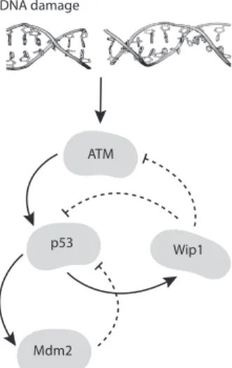
The regulation of p53 is mainly achieved through its interactions with the Mdm2 ligase, that itself is a transcription target for p53. Mdm2 regulates p53 through (multiple-)ubiquitination process, followed by nuclear export and sub-sequent degradation of tagged p53 molecules. Phosphorylation of p53 serine 15 (Ser15) residue, which is located very close to the p53 kinase domain — the target of Mdm2 — can mask it from Mdm2 ubiquitination and hence stabilise it at its highest concentrations [5, 6, 7]. In response to DSBs, p53 can be phosphorylated on Ser15 in three independent ways, among which is phosphorylation by the ATM kinase [7]. Phosphatase Wip1 is another p53 target which acts in the pathway as a regulator; particularly, it dephosphorylates both ATM and p53, rendering them inactive, whence Wip1 closes negative feedback loops between these proteins as is schematically shown on Figure 1.1.

In this article we model and simulate in silico ATM/p53/Mdm2/Wip1

DNA damage

ATM

p53

Mdm2

Wip1

Figure 1.1: The ATM/p53/Mdm2/Wip1 dynamics.

at the single cell level, aiming at further representing cell fate decision in future cell population models. This model is indeed intended to become a first step in narrowing the gap between intracellular and cell population PK–PD models.

Compartmental and spatial p53/Mdm2 models developed by Dimitrio et al. [5, 6]

are here extended by considering the ATM and Wip1 proteins. In these mod-els ATM is interpreted as an identifier of DNA DSBs, although it is not a direct DNA DSB sensor [8]. However, unlike in the originally proposed model, and with the perspective to involve p53 in further PK–PD models, we integrate ATM and

Wip1 into the p53/Mdm2 dynamics so that p53 activation and regulation can be

modelled more plausibly with respect to relevant biological observations. In the

original model, compartmentalisation of cellular events together with p53/Mdm2

feedback (p53 → Mdm2 a 53) led to the desired p53 oscillatory behaviour even with constant ATM parameter (considered as a measure of DNA damage). Under our new assumptions, ATM concentration is considered as a continuous time-dependent function, and we show that the feedbacks p53 → Mdm2 a p53 and AT M → p53 → Wip1 a AT M together with compartmental distribution of pro-teins can then reconstruct the oscillatory dynamics of these propro-teins.

The paper is organised as follows: In Section 2, we give a short biological background of our subject in relation with physiologically based PK–PD mod-elling. Then in Section 3, we present motivations for our modelling work, by firstly describing in detail known mechanisms of p53 activation, p53 activity to-wards its substrates and links between DNA damage and ATM activation. Then

specifications for the proposed model and its computer simulation are presented in Section 4; this section contains our results with their physiological interpreta-tions. Mathematical details, including the complete systems of equations with the parameters chosen for simulations, and some illustrative plots, are presented in the Appendices A to D.

2. Cancer therapies and PK–PD models

Most cytotoxic and cytostatic drugs used in cancer treatments act in a selective

manner, taking advantage of differences in tumour cell characteristics, compared

to healthy cells, such as high proliferation rates, genome instability and tolerance to hypoxia. This results in proper targeting of chemotherapeutic agents on

tu-mour cells. However, cancer therapies also have toxic side effects on healthy cells

and can lead to the disruption of physiological functionality of tissues and or-gans. In the particular case of chronotherapeutic settings (i.e., hypothesizing best treatment periods in the 24 hour span), physiologically based molecular PK–PD models using ODEs have been proposed for the cytotoxic drugs Oxaliplatin [3], 5-Fluorouracil [3, 9] and Irinotecan [10, 11], all three drugs that are commonly used in the treatment of metastatic colorectal cancer. Moreover, to minimise such

unwanted effects in more general (non chrotherapeutic) settings, most anticancer

drugs are delivered in the clinic in time interval-depending regimens to allow cells to recover their normal functions after pharmacological insult. However, time intervals between chemotherapy courses also allow tumour cells to recover, activating their survival mechanisms, and further resist subsequent therapeutic in-sults. Optimal scheduling strategies are currently being theoretically investigated

[2, 3, 12] to obtain satisfying trade-offs between the objective of reducing the

tu-mour burden without inducing neither intolerable side effects on healthy cells nor

emergence of resistant clones in the tumour cell population.

Besides toxic side effects on healthy cells, tumour cells can indeed often

de-velop multiple resistance to drugs. Moreover, in vivo observations in the tumour stromal tissue surrounding tumours of prostate, breast and ovary reveal the drug-induced production of a spectrum of secreted cytokines and growth factors, e.g., WNT16B, that promote tumour growth and survival of cancer cells after cytotoxic therapy, and further reduce chemotherapy sensitivity in tumour cells, resulting in tumour progression; otherwise said, among other constraints, one must take into account the fact that chemotherapy itself can positively influence the growth of tumours [13].

In order to take into account these different therapy-limiting constraints, opti-mal administration of anticancer agents should involve accurately representing the action of drugs at the molecular, i.e., intracellular, level, which means molecular pharmacokinetic-pharmacodynamic (PK–PD) modelling for each drug used in a given treatment firstly at the level of a single cell and secondly (not described in this work) at the level of cell populations, i.e., tissues and organs. The review we present here of p53 molecular mechanisms of action, and their modelling, is po-sitioned in continuity with, but downstream of, the action of cytotoxic anticancer drugs, when DNA damage is constituted, so that DNA damage is the interface between molecular PK–PD models (not recalled here) and the model we propose in Section 4, based on physiological mechanisms reviewed in Section 3.

3. p53 signalling in DNA damage response

Currently, one can find in the scientific literature a large number of papers contributing to describing p53 signalling in detail. In the following sections we point out only the most important facts that are further recalled and used in the model development. Detailed overviews of the p53 transcriptional activity can be found in the works of Murray-Zmijewski et al. [4] and Vogelstein et al. [7]. 3.1. p53 activation and regulation

The tumour suppressor protein p53 can be activated in at least three indepen-dent ways: DNA damage caused, for example, by ionising radiation or electro-magnetic γ radiation, with initial activation of ATM and Chk2 proteins; aberrant growth signals; and various chemotherapeutic drugs, UV radiation and protein– kinase inhibitors. All three ways inhibit p53 degradation and enable the protein to accomplish its main transcriptional function [7].

The concentration of p53 in cells is determined mainly through its degradation. To prevent p53 degradation following DNA damage, ATM (or Chk1, Chk2 and DNA-dependent protein kinases) phosphorylates p53 on Ser15 localised at the amino-terminal sites (in vitro and in vivo) very close to the binding site of its main regulator Mdm2. Phosphorylation of Ser15 masks p53 from Mdm2 (it blocks binding Mdm2 to p53); it stabilises p53 at high concentrations and thus it initiates p53 transcriptional activity [5, 6, 7].

Phosphatase Wip1, a transcription target of p53, is then observed to act in the reverse way, compared with the action of ATM. It dephosphorylates both ATM and p53, making them inactive and unable to phosphorylate their substrates; in

particular, inactive ATM cannot phosphorylate p53 on Ser15 and dephosphory-lated p53 is then detectable by Mdm2, as represented on Figure 1.1 [14, 15, 16].

The E3 ligase Mdm2 is another transcription target of p53. Its p53-inhibiting activity consists in multiple ubiquitination. More precisely, Mdm2 binds the amino-terminus of p53 after Ser15 dephosphorylation and recruits E2 ligases, which directly attach ubiquitines (small peptides) to Lys residues at the carboxyl-terminus of p53. The ubiquitinated p53 protein is then exported to the cytoplasm where it is easily detected by the protein-degrading machinery [7]. Other proteins such as HAUSP can contribute to p53 stability by deubiquitination of p53, i.e. by opposing Mdm2 [4].

Among other things, full p53 transcriptional activation and stabilisation in highly specific situations require other post-translational modifications (phospho-rylation, acetylation, methylation, sumoylation, ubiquitination, etc.) of one or more p53 residues. The particular p53 activity is even more complicated

consid-ering that different modifications of the same p53 residue, e.g. methylation and

ubiquitination of Lys370, result in different p53 effects [4].

3.2. p53 transcriptional activity towards proarrest and proapoptotic proteins The protein p53 as a transcription factor can activate hundreds of genes in re-sponse to a variety of stress signals, thus transforming such signals into various cellular responses. In addition, the p53 transcriptional activity is heterogeneous, depending not only on the incoming signal (its type and amplitude) but also on many other factors — the environment of the cell, type of cells, tissues, presence and abundance of cellular cofactors and enzymes causing modifications of over thirty residues of p53, etc.. All this can induce alterations in p53 stability, expres-sion of substrate genes and cellular location [4].

Experiments on p53 activity on its substrates initially suggested that p53

ac-tivates genes likely with respect to its affinity for a specific promoter. Such

con-ception, for example, assumed that low concentrations of p53 predominantly lead

to the activation of genes of high binding affinity, mostly the genes coding for

proarrest proteins. When the concentration of p53 is high, then it activates also

genes of low binding affinity (i.e. proapoptotic genes). However, this view has

been partially disproved by observations evidencing that post-translational modi-fications contribute to both proarrest and proapoptotic proteins activation without

any preference being due to p53 affinity towards promoters [4]. Recent

experi-ments by Kracikova et al. [1] support these ideas and contradict models based on

proarrest and proapoptotic genes, and that concentrations and durations of the ex-pression of p53 substrates are determined only by concentration and duration of expression of p53 itself.

Importantly, a stressed cell evaluates the presence of both proarrest and pro-apoptotic proteins produced in a p53-dependent manner at any time during its response to DNA damage. The cell determines a so-called “apoptotic ratio” with respect to protein concentrations, duration of their expression and other factors. Irreversible apoptosis launching is initiated whenever this ratio crosses a given threshold [1]. Expression of those apoptosis-launching proteins is a rather com-plex process that depends on many factors (post-translational modifications, in-teractions with other cellular substrates, location, etc.), but from an intracellu-lar PK–PD modelling point of view, the most interesting part, i.e. apoptotic response to therapeutic drugs, must certainly involve p53. However, modelling p53-modulated further cell fate decision (apoptosis or repair and survival, with possible senescence) is omitted from this paper and left for further research,

sim-ply because of so far insufficient biological knowledge of the intracellular (and

intercellular) mechanisms at stake. In this paper, we review, model and simulate the activation and regulation of p53 through the ATM, Wip1 and Mdm2 proteins. 3.3. p53 oscillations in single cells; dependency of such oscillations on ATM

Experiments in individual living breast cancer cells show that concentrations of p53 and Mdm2 exhibit sustained oscillations [17] of duration over several days, with slightly varying period and widely varying amplitude from peak to peak, also

with a number of pulses different from cell to cell, following γ-irradiation [18].

Originally observed damped oscillations that have been measured in immunoblots [19] are likely caused by cancelling of pulses in a population of cells. Note also that not all cells exhibit oscillations in proteins after DNA damage; however, the fraction of oscillating cells increases with the irradiation dose [18].

Further single-cell experiments on the p53/Mdm2 dynamics reveal that the

p53/Mdm2 feedback loop itself is not sufficient to produce sustained oscillations

[14]. Instead, the p53 pulses depend on oscillations of the proteins that sense and transmit the damage signal to p53, particularly ATM and Chk2 (Chk2 itself is a target for ATM), and on the second negative feedback loop between p53 and the phosphatase Wip1, which is schematically illustrated on Figure 1.1. Even thus,

the initial activation of p53 by ATM and Chk2 is not sufficient to generate

mul-tiple p53 pulses, and sustained p53 pulses are detectable in parallel to sustained ATM and Chk2 oscillations only; whenever ATM activity is inhibited, oscillatory behaviour of p53 also vanishes [14].

Hence, although Mdm2 is important for the regulation of p53, Mdm2 without ATM and Wip1 does not lead to p53 oscillations. We thus propose that a model capturing initiation and regulation of p53 activity must involve the ATM and Wip1 proteins, the dynamics of which should be fully described by mathematical vari-ables, solutions of ODEs, rather than represented by constant parameters.

3.4. Compartmentalisation

The p53 protein is a predominantly nuclear protein, which is understandable since its main role consists in the transcriptional activation of many other pro-teins. However, p53 can also play a part outside of the nucleus, notably as a transcription-independent factor involved in apoptosis induction [4, 20]. Note

that there are many cellular substrates affecting p53 location. For example, the E3

ligase E4F1 contributes to stronger association of p53 with chromatin through

multiple ubiquitination, and the PARP1 polymerase positively affects nuclear

accumulation and inhibits nuclear export. On the other hand, Mdm2–mono– ubiquitination of p53 can promote p53 sumoylation with the consequences of

effective p53 nuclear export [4].

ATM is also predominantly concentrated in the nucleus with only 10-20% of its molecules found in the cytoplasm, particularly bound to peroxysomes and endosomes [21]. Fluorescent microscopy techniques have confirmed this spatial distribution of ATM between the nucleus and the cytoplasm. However, only the nuclear fraction of ATM is autophosphorylated in response to DNA damage in-duced by ionising radiation, and activated ATM proteins form detectable foci that are colocalised with foci of γH2AX, a marker of DNA DSBs. Cytoplasmic ATM can neither autophosphorylate itself nor phosphorylate its substrates [22].

The p53-mediated expression of Mdm2 and Wip1 genes produces in the cy-toplasm proteins that can freely migrate between the nucleus and the cycy-toplasm. However, the protein Wip1 is mostly observed to accumulate in the nucleus fol-lowing ionising radiation [23].

3.5. ATM activity on p53

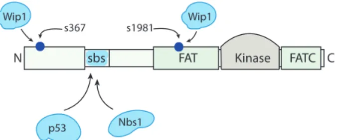
Although p53 activation by ATM in response to DNA damage is well docu-mented, the precise mechanisms of this activation are less well known. We present in Section 3.5.3 an overview of recent biological observations related to the ATM activation and activity. A schematic representation of the ATM protein is shown on Figure 3.1.

N FAT Kinase FATC C

s367 s1981

sbs

p53 Nbs1

Wip1 Wip1

Figure 3.1: Schematic representation of ATM. ATM is a 370 kDa protein with a 350-amino-acid kinase domain between an internal FAT domain, and a carboxyl-terminus FATC domain. ATM substrates such as p53 and Nbs1 bind to a region near the N-terminus (amino acids 1–989) of the protein substrate binding site (SBS). Deletion of SBS inactivates the protein [21]. The nuclear importins α1 and β1 are identified very close to the N-terminus. The N-terminus of ATM is crucial for both nuclear location and chromatin association, optimal ATM activation and subsequent ATM activity in vivo [22]. Wip1 binds to the N-terminus and FAT domain, which contain Ser367 and Ser1981, respectively [16].

3.5.1. ATM activation

In unstressed human cells ATM exists in inactive form as a compound formed (dominantly) from two ATM molecules, which makes it stable in cells, retaining it in a constant concentration, and inaccessible to cellular substrates [24, 25]. In this polymer form, the kinase domain of ATM is bound to a region surrounding Ser1981 that is contained within the FAT domain of ATM, as shown on Figure 3.2. A cell exposure to stress agents (ionising radiation or cytotoxic drugs) induces rapid autophosphorylation of ATM onSer1981 and this phosphorylation results in dimer dissociation and initiation of cellular ATM kinase activity in vivo. In ATM dissociation and activation, the active site of one ATM kinase (one out of two bound in the dimer) catalyses the phosphorylation reaction within which a phosphate group, commonly coming from ATP, is added to Ser1981 of the an-other ATM kinase (resulting in the so called trans-autophosphorylation), shown on Figure 3.2 [24].

Occasional double strand breaks (DSBs) arising, for instance, from DNA replication are normally promptly corrected by the DNA repair machinery, with either no need to activate ATM or such activation being only moderate and tem-porary [26]. After DNA damage caused by other agents (at even as low doses as 0.1 Gy of ionising radiation), ATM activation occurs very promptly [24, 27]. ATM forms clearly detectable foci adjacent to DNA DSBs, and even relatively low

Kinase FAT Kinase FAT Kinase FAT Kinase FAT ATM in an unstressed cell

ATM after DNA damage

phosphate group usually from ATP Ser1981

ATP ATP

Figure 3.2: ATM forming a dimer in an unstressed cell (above) and dimerisation of the dimer into active monomers through autophosphorylation of Ser1981 after DNA damage.

levels of nuclear ATM may be sufficient to elicit proper responses to DNA

dam-age [22]. In addition to exposure of cells to ionising radiation, cytotoxic drugs and restriction enzymes causing DNA DSBs, phosphorylation of Ser1981 and ATM activation is also detectable by introducing chromatin-modifying treatments such as chloroquine or histone deacetylase inhibitors, which do not induce DSBs [24]. 3.5.2. ATM activity

In vivo, ATM activation following ionising radiation occurs very rapidly at distance from DNA DSBs, by means of Ser1981 autophosphorylation. Impor-tantly, the kinetics of p53 phosphorylation on Ser15, and thus p53 activation, cor-responds to the kinetics of ATM activation. Indeed, phosphorylation of p53 is similarly maximal at doses of 1–3 Gy of ionising radiation with little or no further increase up to doses of 30 Gy in fifteen minutes. Clearly detectable p53 phospho-rylation also occurs after employing chromatin-modifying treatments not causing DSBs [24, 27].

In contrast, phosphorylation of the ATM substrates SMC1 (on Ser957), Nbs1 (on Ser343) and H2AX (on Ser139) occurs at the sites of DNA DSBs and in-creases continuously in a dose-dependent manner up to 30 Gy. Furthermore, foci of these proteins are not detectable in case of chromatin modifying treat-ments [24, 27]. In these cases ATM associates with DNA break sites and the ATM attraction to unwinding DNA break ends is modulated by the C-terminus of

Nbs1 [28], a part of the complex of Mre11/Rad50/Nbs1 proteins that actually acts as a sensor of DNA DSBs [8].

Similarly to additional post-translational modifications of p53, ATM contains residues undergoing various modifications, e.g. phosphorylation of the ATM sites Ser367, Ser1893, Ser2996 and Thr1885, that influence various ATM roles in the ATM signalling pathway, mainly at the intra-S phase checkpoint [29, 30]. Acety-lation of Lys3016 by Tip60 has been observed in parallel to Ser1981 phospho-rylation as a crucial event in ATM kinase activation and monomerisation [31]. Inactive or phosphorylation site mutants of ATM fail to bind to DNA DSBs in vivo [32].

3.5.3. ATM regulation

Unlike for p53, the stability of ATM is not determined through its degradation, but rather by reverse association of monomers to dimers (or multimers), i.e. de-phosphorylation of active ATM monomers by some phosphatases and backward dimerisation (multimerisation) of such dephosphorylated monomers.

Abundance and activity of several phosphatases can affect ATM

monomerisa-tion and dimerisamonomerisa-tion, such as phosphatases PP5 [33] and PP2A [34] of the PPP phosphatase family, among which PP2A is likely the only member of this family which can dephosphorylate ATM [34].

Phosphatase Wip1 is also known to dephosphorylate ATM Ser1981 [15]. It has

been shown that inefficient Wip1 results in ATM kinase malfunction, and

overex-pression of Wip1 significantly reduces protein activation in the ATM-dependent signalling cascade after DNA damage. The ATM Ser1981 site is the main tar-get of Wip1 in vivo and in vitro. Moreover, it can dephosphorylate other ATM sites [16]. The protein Wip1 has many other targets in p53 signalling pathway — it dephosphorylates, for example, p53, Chk1 and HA2X.

4. ATM/p53/Mdm2/Wip1 compartmental model

In this section, we design and analyse a mathematical model that can suc-cessfully be used to reconstruct in silico experimentally observed dynamics of proteins, namely, the main cellular actor p53, ATM as a protein transferring the DNA damage signal, Wip1 as a dephosphorylation factor of both p53 and ATM, and Mdm2, that tags p53 for degradation. Note that our model is compartmental in the sense that we strictly distinguish the activities of proteins occurring in the nucleus from those occurring in the cytoplasm, as it is shown on Figure 4.1. Note

also that the model proposed in this section is an extension of the compartmental model developed by Dimitrio et al. [5, 6].

4.1. Model specifications

4.1.1. Modelling ATM activation and deactivation

ATM activation, i.e., its autophosphorylation and consequent dissociation of ATM dimers into (active) monomers, can be modelled in several ways. The sim-plest way is through the dissociation reaction

AT MD

km

k−m

AT Mp+ AT Mp, (1)

where AT MDdenotes a compound of two ATM kinases and AT Mpis active

(phos-phorylated) ATM. In our model, ATM in inactivate state is considered in form of

dimers only. The constants kmand k−m denote, respectively, the monomerisation

(forward) and dimerisation (reverse) rate constants of reaction. Reaction (1)

in-volves monomerisation (dissociation) of a dimer complex AT MDto the two active

ATM species with the rate km and dimerisation of two AT Mp monomers to

pro-duce AT MD with the rate k−m. The law of mass action then gives mathematical

relations between AT MD and AT Mp (not shown), with the production of AT MD

being equal to the half production of AT Mp [35]. A disadvantage of presenting

the activation/deactivation of ATM as in (1), however, is that it does not mention

any signal initiating AT MD dissociation, whereas such a signal is thought to be

produced by changes in chromatin structures after DNA damage [24] and/or by

the MRN complex as a DNA strand breaks sensor [8].

Hence, a more convenient way to represent ATM activation with the perspec-tive of further analysis is to involve a hypothetical, likely molecular and so far unidentified DNA damage signal, that will be denoted by E, produced by DNA damage recognition sensors, transmitted to and sensed by ATM, resulting in the

dissociation of ATM dimers into two molecules of AT Mp, i.e.,

AT MD+ E ki k−i Complex kph2 −→ E+ 2 AT Mp (2)

with the corresponding kinetic rates ki, k−i and kph2. This reaction is not a

typi-cal enzymatic reaction since the enzyme-like signal E is in this approach a non-specified signal corresponding to DNA damage; it is not necessarily an enzyme; however, we assume that E is not amplified, reduced nor otherwise changed in a short time interval.

ATM deactivation by Wip1 is modelled similarly as Wip1+ 2 AT Mp kj k− j Complex−→ AT Mkd ph2 D+ Wip1. (3)

Here, it is assumed that phosphatase Wip1 exists in sufficient concentration to

dephosphorylate ATM active monomers in the sense that whenever one AT Mp

protein is dephosphorylated, another dephosphorylated ATM protein is present, so

that they are immediately bound to the dimeric AT MD. Kinetic rates are denoted

by kj, k− jand kd ph2.

Note that ATM activation and deactivation by Wip1 occur in the nucleus. The law of mass action and the quasi-steady-state approximation [35, 36] then

yield differential equations, hereafter (2) and (3); in particular, changes of

concen-trations in time of AT MDand AT Mpare, respectively,

d[AT MD] dt = −kph2[E] [AT MD] Kph2+ [AT MD] + kd ph2[Wip1] [AT Mp]2 Kd ph2+ [AT Mp]2 , d[AT Mp] dt = 2kph2[E] [AT MD] Kph2+ [AT MD] − 2kd ph2[Wip1] [AT Mp]2 Kd ph2+ [AT Mp]2 , (4)

since the production of AT MD is half that of AT Mp. Here Kph2 =

k−i+kph2 ki and

Kd ph2 =

k− j+kd ph2

kj are the Michaelis-Menten rates of reactions (2) and (3), while

kph2and kd ph2are the velocities of these reactions, [·] denotes concentration.

ATM has not been observed to be degraded during its signalling activity but, after dephosphorylation by Wip1, it rather forms a compound with another ATM dephosphorylated kinase, thus preserving ATM in a stable concentration [24, 32]. Hence, we require ATM to satisfy a conservation property expressing the fact that the total concentration of nuclear ATM kinases (monomers and kinases bound in dimers) is constant during the considered time period, i.e.,

[AT Mp]+ 2[AT MD]= AT MT OT,

where AT MT OT is the constant total ATM concentration. Using this conservation

4.1.2. Modelling p53/Mdm2 negative feedback

The dynamics of p53/Mdm2/Wip1 in the nucleus can be expressed by the

following reactions: p53+ Mdm2 k k− Complex k1 −→ p53U + Mdm2 . . . for p53 ubiquitination by Mdm2, AT Mp+ p53 k2 k−2 Complex−→ p53k3 p+ AT Mp

. . . for p53 phosphorylation by ATM,

Wip1+ p53p

k4

k−4

Complex−→ p53kd ph1 + Wip1

. . . for p53 dephosphorylation by Wip1,

(5)

with the corresponding kinetic constants.

Again, the application of the law of mass action and the quasi-steady-state approximation yields the equations for time changes of the nuclear inactive p53

and active p53p concentrations, i.e.,

d[p53] dt = kd ph1[Wip1] [p53p] Kd ph1+ [p53p] | {z } dephosphorylation of p53pby Wip1 − k1[Mdm2] [p53] K1+ [p53] | {z } ubiquitination of p53 by Mdm2 −k3[AT Mp] [p53] Katm+ [p53] | {z } phosphorylation of p53 by AT Mp d[p53p] dt = k3[AT Mp] [p53] Katm+ [p53] | {z } phosphorylation of p53 by AT Mp − kd ph1[Wip1] [p53p] Kd ph1+ [p53p] | {z } dephosphorylation of p53pby Wip1 . (6)

We do not consider p53 gene expression and its mRNA, since, as it has already been mentioned, the principal means of control on p53 concentration by the cell is through the degradation of the protein, dominantly through the multiple Mdm2-dependent ubiquitination [4]. For simplicity, p53 degradation is rather modelled as an enzymatic reaction and the ubiquitination of p53 in Equation (6) is thus inter-preted as a loss of mass. Note that although p53 degradation controlled by Mdm2 is a preferential way of p53 degradation reported in cells, natural (dominantly cy-toplasmic) degradation also occurs, however, with no significant contribution to

p53 p53 p53_p Mdm2 Wip1 Wip1 Mdm2 ATMp ATM Wip1 Wip1 Mdm2 Mdm2 RNA RNA RNA RNA

Figure 4.1: Assumptions on the location and exchange of considered proteins between the nucleus and the cytoplasm made in our model. mRNA variables are denoted on this figure by the additional subscript RNA, and similarly the subscript

p denotes a phosphorylated protein. The proteins p53 and Mdm2 are assumed

to migrate freely (i.e., without diffusion limitations, resulting in homogeneous

concentrations) within each of the two compartments, nucleus and cytoplasm.

the overall p53 degradation [37, 38]. Thus, in parallel to Mdm2 ubiquitination la-belling of p53, we add a normal decay term for the degradation of the cytoplasmic p53.

The genes coding for Mdm2 and Wip1 are expressed in a p53-dependent man-ner, and we have chosen to model the transcription of these genes quite classically,

by using a Hill function with coefficient 4, since the transcriptionally active p53

appears in tetrameric form [39]. Note that other choices of the coefficient can

be used; however, different Hill coefficients may result in different dynamical

re-sponses of the studied system. Denoting the basal Mdm2 mRNA production rate

kS m, the protein transcription of the Mdm2 gene to its mRNA, Mdm2RNA, can be

written as d[Mdm2RNA] dt = kS m+ kSpm [p53p]4 [p53p]4+ K_S4_pm | {z } Mdm2 gene transcription . (7)

The mRNA of Mdm2 then moves to the cytoplasm where it is translated.

Trans-lation is modelled as a linear process with the constant transTrans-lation rate ktm. Note,

however, that the equations for the cytoplasmic concentrations of mRNAs, Equa-tion (B.2) in the appendix, describe the concentraEqua-tions of the unbound mRNAs present in the cytoplasm. In other words, the mRNA of Mdm2 (similarly, the mRNA of Wip1) already used in translation is modelled as a loss of the free mRNA available in the cytoplasm, and thus it is subtracted from the total mRNA. Produced protein Mdm2 can then freely migrate between the cytoplasm and the nucleus, and ubiquitinate p53 in both compartments (the equation for p53 in the cytoplasm is designed in the same way as for the p53 nuclear equation). Regula-tion of Mdm2 is represented only by considering degradaRegula-tion terms for Mdm2

and Mdm2RNA. The constants kSpm and KSpm are, respectively, p53-dependent

Mdm2 mRNA transcription velocity and Michaelis-Menten p53-dependent Mdm2 mRNA transcription rate.

Transcription and translation of the Wip1 gene run similarly with the

corre-sponding reaction constants kSpw and KSpw, the production rate kS w, and the

trans-lation rate ktw. Note, however, that Wip1 has been observed to be a predominantly

nuclear protein [23]; for this reason, unlike Mdm2, the Wip1 protein has been as-sumed to move only to, and not from, the nucleus. Phosphatases other than Wip1 that can dephosphorylate ATM and p53 have not been considered in the model.

The compartment-specific physiological roles of the proteins, already men-tioned in Section 3.4, translate into mathematical simulations in the model that explicitly take into account cell compartmentalisation. Our assumptions about the location of these proteins are shown on Figure 4.1.

Most of the kinetic velocities and Michaelis-Menten constants (Table B.1 in Appendix) appearing in the reactions are taken from the sicentific literature on the subject [5]; ATM and p53 dephosphorylation rates by Wip1 are taken from works of Shreeram et al. [15, 16]. Other unknown parameters (in Wip1 expres-sion, ATM activation) are chosen by exploring the space of parameters so that the system exhibit oscillatory dynamics for the proteins. These biological observation facts, together with linear or Michaelis-Menten degradation terms, and boundary conditions on protein exchanges through the nucleocytoplasmic membrane (their

fluxes being taken as proportional to the differences between averaged nuclear and

cytoplasmic concentrations [5, 6]), finally result in the ODE system that is solved numerically (equations B.1 and B.2 in Appendix).

4.1.3. Short overview of other existing models

There are several mathematical models describing the p53/Mdm2 dynamics,

for example the already mentioned models by Lev Bar-Or et al. [19] which show (experimentally and numerically) the presence of damped oscillations. The model developed by Batchelor et al. [14], which is actually based on former models by Geva-Zatorsky et al. [18], includes only nuclear concentrations of proteins. Ma et

al.[40, 41] use delay differential equations (DDE) to simulate particular delays in

representing the transcription of Mdm2 mRNA and translation of Mdm2 mRNA into the Mdm2 protein. Their models contain p53 activation by ATM kinase and only nuclear species are considered.

Ciliberto et al. [42] use the negative feedback p53 → Mdm2 a p53

supple-mented by a simplified positive feedback to reconstruct p53/Mdm2 oscillations.

In the positive feedback, p53 initiates activation of a cascade of protein interac-tions (involving PTEN, PIP2, PIP3 and Akt) leading to temporal inhibition of cytoplasmic Mdm2 translocation to the nucleus. T. Zhang et al. [43] explore the

mechanism of p53/Mdm2 network of [42] and offer three other models

simulat-ing p53/Mdm2 dynamics which combine different positive feedbacks with the

p53/Mdm2 negative feedback. In addition, they propose a mechanism enabling

a cell to decide between cell cycle arrest and apoptosis, assuming that persistent p53 pulses trigger apoptosis. X.P. Zhang et al. [44] combine results of [42, 43] and

develop a two-phase switch model, which includes p53/Mdm2, ATM/p53/Wip1

and p53/PTEN/Akt/Mdm2 feedbacks, and which can simulate irreversible

transi-tion from cell cycle arrest to apoptosis. Both models of [43, 44] simulating cell fate decision involve transcription of proarrest and proapoptosis proteins p21 and p53DINP1 (and other proteins), respectively, the activation of which, however, is

regulated by the p53 affinity for the protein genes, i.e., proarrest proteins are

pro-duced initially in an early cell response phase to DSBs, and proapoptotic proteins are produced later after a few p53 pulses. Note that the transcriptional regulation

of proteins is modelled by using Hill functions, mostly with coefficients 3 and 4,

in all the mentioned works [40, 41, 42, 43, 44].

There are also some other models simulating p53 signalling network, for ex-ample, a recently proposed deterministic model by J.K. Kim and T.L. Jackson [45] with the positive feedback between p53 and Rorα and a model proposed

by K. Puszy´nski et al. [46] taking stochastic effects into account. Sturrock et

al. [47, 48, 49] and Dimitrio et al. [5, 6] study p53/Mdm2 dynamics, without

Wip1, but using PDE spatial models with exchanges through the nucleocytoplas-mic membrane, ATM being considered in Dimitrio et al. as a bifurcation

parame-(a) 0 6 12 18 24 0 0.5 1 1.5 2 time (hrs) dimensionless concentration [ATM_p](n) [p53 p] (n) [Mdm2](n) [Wip1](n) (b) 0 6 12 18 24 0 0.2 0.4 0.6 0.8 1 1.2 1.4 time (hrs) dimesnionless concentration [ATM D] [ATM p]

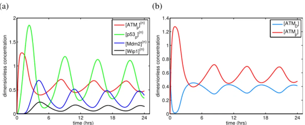
Figure 4.2: (a) Nuclear ATM/p53/Mdm2/Wip1 oscillations over a 24 hour-long

time interval. (b) Evolution of the ATM monomerisation and dimerisation with

the total concentration of ATM, AT MT OT(0)= 1.3µM, and [E] = 0.1µM (where E

is a hypothetical damage signalling molecule launching ATM activation). Plotted concentrations are dimensionless.

ter; both models exhibit sustained oscillations for p53. 4.2. Numerical simulations and discussion

4.2.1. The ODE model reproduces the pulsatile behaviour of proteins

Under specified circumstances, the model ODE system yields expected pul-satile behaviour for the proteins. Pulses of the involved proteins are illustrated on Figure 4.2. Figure 4.2(a) confirms that the model can be used to reconstruct experimental observations [14]. After DNA damage producing a (likely

molec-ular) signal E with concentration [E] = 0.1µM (in this particular simulation),

ATM is firstly activated. Then AT Mp phosphorylates p53 and thus, the peak on

the curve of p53p evolution is observed later than the peak of AT Mp. Mdm2 and

Wip1 are the targets of active p53p, hence the corresponding peaks appear after

the p53 peak. Mdm2 and Wip1 then regulate p53, which leads to p53p

dephos-phorylation and degradation. Wip1 also dephosphorylates AT Mpwith formation

of ATM dimers. The period of the first pulse for nuclear p53p is ∼5.16 hours and

for AT Mp, it is ∼4.4 hours, which fits experimental observations [14, 17]. ATM

evolution can be seen on Figure 4.2(b). The amount of activated AT Mp at the

peaks of the evolution curve exceeds 50% of all ATM protein, as has been ob-served in biological experiments [24]. Note that the total concentration of ATM is

(a) 0 0.5 1 1.5 0 0.5 1 1.5 2 ATM_p p53 p (b) 0 0.2 0.4 0.6 0.8 1 0 0.2 0.4 0.6 0.8 1 1.2 1.4 1.6 1.8 2 Mdm2 p53 p

Figure 4.3: Phase plane curves relative to the involved nuclear proteins with [E] =

0.1µM (where E is a hypothetical damage signalling molecule launching ATM

activation): (a) AT Mpand p53p(b) Mdm2 and p53p.

The pulses of the proteins on Figure 4.2 are, apart from a couple of first pulses, of the same amplitude, i.e., the model quickly produces sustained (undamped) oscillations [14, 17]. This can be seen from the phase plane Figures 4.3 (and Figures E.1 in the Appendix), showing orbits of the solutions fastly converging toward stable limit cycles. The first pulses on Figure 4.2(a) are of higher ampli-tude mainly because of the choice of initial concentrations of proteins; all initial concentrations of proteins are set to be zero in our simulations, and since Wip1 and Mdm2 are not initially present in the cell, the concentrations of p53 and ATM increase until the regulators Wip1 and Mdm2 start to accumulate in the nucleus and thus inhibit further p53 and ATM production.

The proposed ODE model is “noise-free” and we do not consider stochasticity in protein gene expression, nor noise in protein production rates. The ampli-tudes of experimentally observed pulses in the extended research works of Geva-Zatorsky et al. [18] are found to vary widely from peak to peak and from cell to cell (even within the same irradiation dose), mainly due to noise in protein produc-tion rates. It is also worth menproduc-tioning that the periods of biologically measured

oscillations are affected by noise, so that the duration of one pulse may be

differ-ent from another; however, this difference comes with a variability of (at most)

20% in contrast to the 70% variability in amplitudes [18]. Our ODE model shows

variability in periods in the first couple of pulses, simulated with [E] = 0.1µM

(Figure E.2(a) in the Appendix). The first pulse is of length 5.16 hours, the period

impact of noise on oscillations for further modelling works.

4.2.2. Bifurcation analysis of the system reveals two supercritical Hopf bifurca-tion points that correlate with DNA damage levels

(a) 0.01 0.014 0.016 0.018 0.02 H H −2 −1 0 1 2 3 x 10−3 −0.022 −0.02 −0.018 −0.016 −0.014 H H Re Im (b) −5 −4 −3 −2 −1 0 5.9 5.95 6 6.05 6.1 6.15 6.2 6.25 6.3 6.35 log 10E

periods of stable limit cycles (hrs)

H

H

Figure 4.4: (a) Pair of eigenvalues crossing the imaginary axis for [E]= 2.5×10−5

and [E] = 0.97 and thus revealing Hopf bifurcation points. (b) Evolution of

the period of the stable limit cycles occurring between the two Hopf bifurcation points; [E] is in logarithmic scale.

With [E]= 0 we can easily calculate the equilibrium point of the studied

sys-tem (not shown). Forward continuation, using the Matlab package MatCont [50], of the equilibrium curve starting from the previously computed equilibrium point,

numerically reveals two Hopf bifurcation points with negative Lyapunov coe

ffi-cients [51] p. 120, i.e., corresponding to supercritical Hopf bifurcations. These

Hopf bifurcation points are obtained for the values [E]1 = 2.5 × 10−5µM and

[E]2 = 0.97µM. Note that the computed equilibria are hyperbolic, [51] p. 67,

ex-cept for the two Hopf bifurcation points, since the Jacobian matrix of the system

has eigenvalues with non-zero real parts for all values of [E] except [E]1and [E]2.

A special situation appears in case of the Hopf points where a pair of complex

eigenvalues crosses the imaginary axis, see Figure 4.4(a). For values below [E]1

the equilibrium of the system is stable (all eigenvalues have negative real parts) and the concentrations of proteins tend to their steady states very quickly. By passing through this value, the equilibrium becomes unstable (the pair of com-plex eigenvalues crossing the imaginary axis change the real parts from negative to positive) and stable limit cycles appear; the equilibrium of the ODE system is

The periods of the stable limit cycles vary between 5.92 and 6.26 hours with

varying [E], as illustrated on Figure 4.4(b). Bifurcation diagrams of p53pwith

re-spect to E, p53p/AT Mp, p53p/Mdm2 and p53p/AT Mpare plotted on Figures 4.5.

The amplitudes of p53pand AT Mp of the stable limit cycles are small for values

of [E] close to [E]1and [E]2, respectively (as expected in the case of supercritical

Hopf bifurcations), which is illustrated on Figures 4.5(a) and 4.5(b). This does not, however, mean that the amplitudes of concentrations are of such small values throughout the whole time period. In fact, it may take several days until the limit cycle is reached; compare, for example, Figures 4.5(a) with 4.6(a) and 4.6(b).

In our ODE settings, E is considered as the measure of DNA damage. Inter-esting situations appear whenever E is small and close to the first Hopf bifurcation point (which may correspond to a few DSBs only) and when E is very big (which may correspond to serious DNA damage and many DSBs). In the first case, the

AT Mp solutions do not even oscillate for the values of [E] ≈ [E]1. The ATM

trajectories then tend to steady states with low values; however, these small

con-centrations of AT Mp can still elicit p53p pulses, see Figure 4.6(a). This may

contradict experimental observations that show ATM oscillations accompanying p53 oscillations after DNA damage [14]; note, however, that those experiments were performed with exposure of cells to 10 Gy of γ-irradiation and did not con-sider that DNA damage can cause only a few DSBs (and which may correspond to

[E]1). On the other hand, other works show evidence that only very small amounts

of ATM (even not detectable) can still elicit actual p53 signalling [22, 26]. Indeed,

DNA damage at [E] ≈ [E]1 may correspond to occasional DNA DSBs which do

not need ATM for DNA repair and only moderate ATM is produced which is still

efficient in p53 activation.

ATM oscillations are damped and disappear for [E] greater than [E]2: once the

oscillations have vanished, they do not appear again with further increasing values

of [E]. Figure 4.6(b), for example, shows the protein dynamics for [E] = 10µM.

In this case ATM is almost fully activated and only small deviations in ATM con-centration can be seen. Hence, we can speculate that if it is impossible to re-pair DNA DSBs, then phosphatase activities on ATM are inhibited, active ATM achieves its maxima and apoptosis is initiated. However, the latter suggestion is not supported by experimental observations; in fact, there is no paper in the liter-ature, to our best knowledge, clarifying ATM activity and location in single cells committing apoptosis. Thus, ATM oscillates whenever it is necessary for a proper cell response to DNA damage of an alive cell, and once [E] becomes too high, os-cillations disappear and the cell is sent to apoptosis and dies. Such interpretation, however, requires E to be dependent not only on DNA damage levels but also

(a) −4 −3 −2 −1 0 0 0.5 1 1.5 2 log 10E p53 p H H (b) −4 −3 −2 −1 0 0 0.5 1 1.5 log₁₀E ATM p H H (c) 0 0.1 0.2 0.3 0.4 0.5 0.6 0 0.5 1 1.5 Mdm2 p53 p _H H (d) 0 0.2 0.4 0.6 0.8 1 1.2 0 0.5 1 1.5 ATM p p53 p H H H H

Figure 4.5: (a) Bifurcation diagram for nuclear p53p, (b) bifurcation diagram for

nuclear AT Mp with respect to E = [E], E is in logarithmic scale. Bars plotted

on figures are the heights (showing maximum and minimum) of the amplitudes

of stable limit cycles. (c) p53p/Mdm2 limit cycles occurring for values of the

damage signal E between the two Hopf bifurcation points. (d) The same in the

p53p/AT Mp phase plane. Plotted concentrations are dimensionless. The

equilib-rium curves in (c) and (d) are the curves joining the two Hopf bifurcation points H, constituting stable, then unstable, and then stable equilibrium branch again, with the stable limit cycles surrounding the unstable equilibrium points.

(a) 0 6 12 18 24 30 36 42 48 0 0.1 0.2 0.3 0.4 0.5 time (hrs) dimensionless concentration [ATM p] (n) [p53 p] (n) (b) 0 6 12 18 24 0 0.5 1 1.5 2 time (hrs) dimensionless concentration [ATM_p](n) [p53 p] (n) [Mdm2](n) [Wip1](n)

Figure 4.6: (a) Nuclear p53p/AT Mp concentrations from the ODE system for

[E]= [E]1 = 2.5×10−5µM. The concentration of AT Mpconverges to the

equilib-rium point and the concentration of p53ptends to a stable limit cycle. (b) Nuclear

AT Mp/p53p/Mdm2/Wip1 concentrations for [E] = 10µM. The concentration

of AT Mp is of small amplitude, getting even smaller with further increasing [E].

Plotted concentrations are dimensionless, AT MT OT(0)= 1.3µM.

on other factors amplifying the abundance of E, possibly with the contribution of proapoptotic proteins. Indeed, Figure 4.6(b) still shows (damped) p53 pulses, initially of higher amplitudes, that can act transcriptionally on its substrates. 4.2.3. Two negative feedback loops and a compartmental distribution of cellular

processes produce sustained oscillations

In order to prove that the oscillating ATM protein plays an active role in

achieving p53 pulses we made several simulations to test different possibilities

and thus we explored the system in more details. For example, the model can

be used to mimic the observed inhibition of p53/Mdm2 pulses following one full

ATM pulse [14]; this is illustrated on Figures 4.7, where ATM is inhibited after one pulse. We can see the complete first pulses of ATM, p53, Mdm2 and Wip1, among which protein Wip1 blocks further ATM activation (in the corresponding equation (4) of ATM dephosphorylation by Wip1, the Michaelis-Menten constant Kd ph2 is set to be very small, Kd ph2 = 0.0001). Although the first pulses of the

p53 and Mdm2 proteins are induced, they are not sufficient to produce subsequent

pulses after ATM dissociation is blocked. Other tests when we inhibit, respectively,

(a) 0 6 12 18 24 0 0.2 0.4 0.6 0.8 1 1.2 1.4 time (hrs) dimensionless concentration [ATM_p](n) [p53 p] (n) [Mdm2](n) [Wip1](n) (b) 0 6 12 18 24 0 0.2 0.4 0.6 0.8 1 1.2 1.4 time (hrs) dimesnionless concentration [ATM D] [ATM p]

Figure 4.7: (a) The nuclear ATM/p53/Mdm2/Wip1 dynamics over a 24 hour-long

time interval following ATM inhibition after one full pulse. (b) Evolution of the ATM monomerisation and dimerisation with the total concentration of ATM,

AT MT OT(0)= 1.3µM, and [E] = 0.1µM, following ATM inhibition after one full

pulse. Plotted concentrations are dimensionless.

Appendix),

• the positive feedback AT M → p53 (k3 = 0 in (6), Figure E.3(b)),

• the negative feedback Wip1 a p53p(kd ph1 = 0 in (6), Figure E.3(c)),

• the positive feedback p53p → Wip1 (kSpw = 0, Figures E.3(d) and (e)),

produce either damped oscillations or do not produce oscillations at all. The ATM

and Wip1 proteins must thus be involved in the p53/Mdm2 dynamics in order to

produce sustained p53 oscillations.

The p53/Mdm2 negative feedback cannot be omitted either, since the

inhibi-tion of Mdm2 activity on p53 (k1 = 0 in (6), see Figure 4.8(a)) or the inhibition

of the transcriptional activity of p53p on Mdm2 (kSpm = 0 in (7), Figures E.3(f)),

does not produce oscillations.

We can further ask whether the two feedback loops without strict location of proteins in the compartments can lead to p53 oscillations. Merging protein dy-namics into one compartment (the whole cell), i.e. omitting exchange of proteins between the nucleus and the cytoplasm but rather considering both compartments as the one where proteins and their mRNA can freely migrate, is not, however,

protein concentrations in the case [E] = 0.1µM. As in the case shown on this figure, all other choices of [E] exhibit concentrations of proteins converging to their steady states (bifurcation analysis does not reveal any significant point). The role of compartmentalisation in p53 dynamics has been studied in more details in another research work [5, 52].

Hence, the feedbacks p53 → Mdm2 a p53 and AT M → p53 → Wip1 a

AT Mtogether with compartmental distribution of proteins result in sustained

os-cillations, and neglecting any part of these three components fails to produce sus-tained oscillations. (a) 0 6 12 18 24 0 0.5 1 1.5 2 2.5 3 time (hrs) dimensionless concentration [ATM_p](n) [p53 p] (n) [Mdm2](n) [Wip1](n) (b) 0 6 12 18 24 0 0.5 1 1.5 2 time (hrs) dimensionless concentration [ATM_p](n) [p53 p] (n) [Mdm2](n) [Wip1](n)

Figure 4.8: (a) The ATM/p53/Mdm2/Wip1 dynamics over a 24 hour-long time

interval, [E] = 0.1µM, in a case when Mdm2-mediated ubiquitination of p53

is inhibited, k1 = 0. (b) The ATM/p53/Mdm2/Wip1 dynamics over a 24

hour-long time interval and [E] = 0.1µM in a case when only one compartment is

considered.

4.2.4. ATM threshold required for initiation of p53 pulses

Note again that there are two significant points in the range of the signal E,

the two Hopf bifurcation points, [E]1 = 2.5 × 10−5µM and [E]2 = 0.97µM in

the presented simulation settings: values of E starting from [E]1 are sufficient

to elicit sustained oscillations in the p53 protein nuclear concentrations, and the

second Hopf bifurcation point [E]2is the critical point at which stable limit cycles

(otherwise said, sustained oscillations of the proteins) disappear. This point thus may mark a decision for the cell not to go on in DNA DSBs repairing processes, and rather to start apoptosis. A relation to a supposed apoptotic threshold [1] remains however to be further established.

The hypothetical signal E is supposed to be produced by DNA DSB sensors

and/or by changes in chromatin structure, and may be affected by other factors like

the MRN complex bound to the DNA break sites and the presence of proarrest and proapoptotic proteins. Then E is delivered to ATM dimers and promotes

ATM activation. Interestingly, an amount of E as small as [E]1 can, for a value

of the total ATM protein AT MT OT = 1.3µM, activate ATM at the concentration

∼0.02µM, Figure 4.6(b), that is sufficient to produce oscillations in p53.

Note, however, that the Hopf bifurcation points are dependent on the total

concentration of nuclear ATM, AT MT OT. Indeed, Figure 4.9(a) shows the

evo-lution of the Hopf bifurcation points with respect to AT MT OT (on the y-axis).

We can see that the values of [E]1 do not change dramatically and they range

between 1, 17 × 10−5 (which corresponds to AT MT OT = 10µM) and 3.5 × 10−5

(which corresponds to AT MT OT = 0.78µM). The dependence of [E]2on AT MT OT

seems to be more intriguing. Similarly to [E]1 the Hopf bifurcation points [E]2

increase with decreasing AT MT OT, and asymptotically reach values

correspond-ing to AT MT OT ≈ 0.77µM, Figure 4.9(a). In other words, the system has two

Hopf bifurcation points for AT MT OT > 0.77µM (with similar bifurcation

dia-grams between these points Figure 4.9(b)); the only one Hopf bifurcation point

∼3.8 ×105 _{below AT M}

T OT = 0.77µM determining stable solution and unstable

solution (stable limit cycle). The system does not have any Hopf bifurcation point

for AT MT OT < 0.082µM.

Interestingly, for all the [E]1 values corresponding to different AT MT OT, the

concentration in activated ATM protein always reaches the steady-state value 0.02µM (not shown). This helps resolve a biological unanswered question; in particular, it has been observed that only a fraction of ATM molecules can be suf-ficient to initiate proper cell responses to DNA damage [22]; however, a certain threshold for initial ATM concentration is supposed to exist (but it is not speci-fied) to initiate the ATM signalling pathway [14]. Thus, the analysis of our model reveals that the threshold for ATM, which is independent of the total nuclear ATM proteins, can be 0.02µM (in our model constant settings).

5. Conclusion

Explaining experimentally observed p53 oscillations in human cancer cells after exposure of the cells to γ-irradiation [14, 17, 18] is a mathematical mod-elling challenge, especially in the perspective of proposing p53-mediated

anti-cancer drug-induced cell cycle arrest/apoptotic predictions. This paper is the

(a) −60 −4 −2 0 2 4 6 8 10 log 10 E ATM TOT [E]2 [E]1 [E]2 [E]1 (b) −5 0 0 5 10 0 0.5 1 1.5 2 H log₁₀ E H H H ATM_TOT p53 p

Figure 4.9: (a) The evolution curves of both Hopf bifurcation points (curves in

brown and black colours). The Hopf bifurcation points [E]1 and [E]2 are

com-puted for AT MT OT = 10µM, the points [E]1 and [E]2 for AT MT OT = 0.78µM.

The concentration E = [E] is in the logarithmic scale. (b) Bifurcation diagrams

of p53pwith respect to changing AT MT OT and [E].

“guardian of the genome” p53, that plays essential parts in cell responses to DNA damage and checkpoint signalling. The spatial distribution of proteins in a cell is taken into account and it is shown that such compartmental recognition of cellular events allows to reconstruct the pulsatile behaviour of proteins without the need to introduce any time delay in their dynamics.

The oscillatory dynamics of the involved proteins can be speculatively ex-plained as periodical testing of the presence of DNA damage; if unrepaired DNA DSBs still exist, additional pulses of both phosphorylated ATM and p53 are trig-gered. More precisely, we propose the following interpretation: the level of phos-phorylated ATM increases in response to DSBs and is then reduced due to the in-crease of the p53 concentration (since ATM phosphorylation of p53 leads to p53 stabilisation, which, afterwards, activates Wip1, that inactivates ATM). When p53 levels are in turn reduced by the interaction with Mdm2 (after p53 dephosphory-lation by Wip1), ATM is released to re-examine the DNA. If the number of breaks remains above a certain threshold, the pathway becomes reactivated, leading to a second pulse of ATM and p53, and this continues until the number of DNA breaks is dropped below the threshold, or the cell decides to start apoptosis [14].

The original models of Dimitrio et al. [5, 6] involve ATM as a direct mea-sure of DNA damage, in the form of a parameter that remains constant in the

studied time interval. It has been experimentally shown, however, that a pulsatile

behaviour for p53/Mdm2 cannot be achieved without oscillations of ATM [14].

In addition, there exist biological studies that confirm a role for ATM in cancer cell apoptosis induced, for example, by ionising radiations [53]. Hence, in this ex-tended modelling work, we consider ATM as an essential part of the DNA damage signalling pathway, varying with time, that after ATM dimer dissociation and ac-tivation, phosphorylates p53 and thus initiates p53 transcriptional activity towards proarrest and proapoptotic genes (for example, p21 and 14-3-3σ on the proarrest side, and Pig3, Apaf1 and PUMA on the proapoptotic side).

The p53 protein responds to a variety of cellular stresses (such as those causing DNA strand breaks, e.g., cytotoxic drug insults) through the transcription mode of protein production. Despite the complexity of all signalling pathways occur-ring in the stressed cells and the production of proteins involved therein, we can conclude that the pathway including p53 activation can be successfully recon-structed by our compartmental model that, in particular, takes into account the

ATM/p53/Mdm2/Wip1 pulsatile dynamics as has been observed in the scientific

literature on the subject [14, 15, 24, 26], and as is summarised in details in the biological background part of the present work.

In an even more realistic vision of the processes leading a single cell to de-cision between survival and death, more than on deterministic events, random molecule encounters and stochastic gene expression should be taken into consid-eration, and should be modelled by stochastic processes (as sketched in [49] for

Hes1), from which deterministic equations (partial differential equations

physi-ologically structured in variables, identified as biological “readouts” in a single cell model, representing relevant biological variability inside the cell population) should be further designed at the level of cell populations.

In the same way, in the perspective of connecting the proposed p53 modelling

with existing PK–PD models, drug effects, measured only at the cell

popula-tion level, can be represented as environmental factors exerting their influence on molecular targets, included as functions in stochastic processes, at the level of a single cell. Establishing such connections between stochastic events at the

indi-vidual cell level and resulting deterministic effects at the cell population level is

a challenge for mathematical modelling that we intend to tackle in future works. Readers interested in such interconnections between stochastic and deterministic mathematics in the Hes1 regulatory network are recommended to read the papers by M. Sturrock et al. [49, 56] to get acquainted with this challenge, a considerable one in the most general case.

Appendix A. Equations for ATM dynamics

Following in vivo observations [24], ATM is activated very shortly after DNA damage in the nucleoplasm, i.e., with no need of ATM binding DNA damage

sites, through the dissociation of the inactive ATM dimers, AT MD, into the active

monomers, AT Mp. The activation signal is however not biologically specified; it

is assumed to be produced by changes in chromatin after DNA damage [24, 27], amplified by MRN complex (sensor of DNA DSBs) [54], or this signal may be actually the MRN complex itself and its interaction with ATM [55]. Although there is not a general agreement among biologists, ATM is mostly thought to be activated very promptly. We thus represent ATM activation through its interaction with an unknown signal, likely a molecule or the result of a chain of molecular reactions, denoted by E, which is assumed to be constant in a very short time interval, so that the reaction of E with ATM dimers can be written as the enzymatic reaction, Equation (2), i.e.

E+ AT MD

ki

k−i

Complex−→ 2 AT Mkph2 p+ E. (A.1)

Dephosphorylation (and deactivation) of ATM monomers is observed through the

interaction of AT Mpwith Wip1 [14, 15, 16], Equation (3), i.e.

Wip1+ 2 AT Mp

kj

k− j

Complex−→ AT Mkd ph2 D+ Wip1. (A.2)

By applying the law of mass action and the quasi-steady-state approximation,

the loss of AT MDderived from the first reaction (A.1) can be written in the form

d[AT MD]

dt = −kph2[E]

[AT MD]

Kph2+ [AT MD]

. (A.3)

However, the equation for the loss of AT Mpis not so straightforward, since as

a substrate we now have two AT Mp proteins. Let us write

s= [AT Mp], e = [Wip1], p = [AT MD] and c= [Complex]

for the concentrations of the reactants in (A.2). Then the law of mass action applied to (A.2) leads to the following equation for the substrate s,

ds

dt = −2kjs

2_{e+ 2k}

since in every c that is made, two of s are used, and every time c is degraded, two of s are produced; and for the other reactants,

de dt = −kjs 2 e+ (k− j+ kd ph2)c, dc dt = kjs 2 e −(k− j+ kd ph2)c, d p dt = kd ph2c. (A.5)

The initial conditions are e(0) = e0, s(0) = s0 and c(0) = p(0) = 0. With the

conservation property of the enzyme e, de_dt + dc_dt = 0, and so with e(t) = e0 − c(t),

we have the system of ordinary differential equations (ODEs) reduced to

ds dt = −2kjs 2 (e0− c)+ 2k− jc, dc dt = kjs 2_(e 0− c) − (k− j+ kd ph2)c. (A.6)

The quasi-steady-state approximation then assumes dc_dt ≈ 0. Hence, from the

second equation in (A.6) we can explicitly write c in terms of s, in particular,

c= e0s 2 s2+ K d ph2 (A.7) where Kd ph2 = k− j+kd ph2

kj is the Michalis-Menten rate of reaction. Substituting c in

the equation for s, we finally can write ds dt = −2e0kd ph2 s2 s2+ K d ph2 , (A.8)

where in numerical simulations e0 is replaced by e.

By coming back to our original problem reaction (A.2), we get the equation

for the loss of AT Mp,

d[AT Mp]

dt = −2kd ph2[Wip1]

[AT Mp]2

[AT Mp]2+ Kd ph2

. (A.9)

and deactivation. In particular, equations of interest are d[AT MD] dt = −kph2[E] [AT MD] Kph2+ [AT MD] + kd ph2[Wip1] [AT Mp]2 Kd ph2+ [AT Mp]2 , d[AT Mp] dt = 2kph2[E] [AT MD] Kph2+ [AT MD] − 2kd ph2[Wip1] [AT Mp]2 Kd ph2+ [AT Mp]2 , (A.10)

since the production of AT MD is half of AT Mp. Note that we do not consider

ATM in inactive monomeric state.

Note that it is, however, not necessary to use both equations in numerical sim-ulations, and actually, we cannot use both of them, since the Jacobian matrix of

the ODE system composed of all other equations describing the p53/Mdm2

dy-namics, see Appendix B, is singular for [E] = 0, i.e. for the value for which

the system achieves equilibrium. This is because the derivative of the right-hand

side of the first equation in (A.10) with respect to the variable [AT MD] is zero

for [E]= 0, similarly the derivatives of all other right-hand sides of the equations

describing the dynamics of proteins are zeros as well (simply because these

equa-tions do not contain [AT MD], i.e. they are constants with respect to [AT MD]);

see the equations in (B.1) and (B.2). To calculate the equilibrium for [E] = 0 is

a straightforward algebraic exercise; the problem, however, is in the continuation

of the equilibrium curve starting at the computed equilibrium for [E] = 0, since

continuation techniques require non-singular Jacobian matrices.

By recalling the conservation property of the ATM protein, i.e. [AT Mp] +

2[AT MD]= const = AT MT OT [µM] and thus by writing [AT MD]= 1₂(AT MT OT −

[AT Mp]) in the second equation in (A.10), we actually have the mathematical

equation for [AT Mp] in the form

d[AT Mp] dt =2kph2[E] 1 2(AT MT OT − [AT Mp]) Kph2+ 1₂(AT MT OT − [AT Mp]) − 2kd ph2[Wip1] [AT Mp]2 Kd ph2+ [AT Mp]2 . (A.11)

The conservation property observed by Bakkenist and Kastan [24] claims (almost) non-changing concentration of the total ATM proteins. Note that ATM is not observed to be degraded in the cell and since it is the 370 kDa large protein, its inactivation through the dimerisation instead of degradation is energetically more profitable.