Mixed-Integer Benchmark Problems for Single-and Bi-Objective Optimization

(1)

HAL Id: hal-02067932

https://hal.inria.fr/hal-02067932

Submitted on 14 Mar 2019

HAL is a multi-disciplinary open access

archive for the deposit and dissemination of

sci-entific research documents, whether they are

pub-lished or not. The documents may come from

teaching and research institutions in France or

abroad, or from public or private research centers.

L’archive ouverte pluridisciplinaire HAL, est

destinée au dépôt et à la diffusion de documents

scientifiques de niveau recherche, publiés ou non,

émanant des établissements d’enseignement et de

recherche français ou étrangers, des laboratoires

publics ou privés.

Mixed-Integer Benchmark Problems for Single-and

Bi-Objective Optimization

Tea Tušar, Dimo Brockhoff, Nikolaus Hansen

To cite this version:

Tea Tušar, Dimo Brockhoff, Nikolaus Hansen. Mixed-Integer Benchmark Problems for Single-and

Bi-Objective Optimization. GECCO 2019 -The Genetic and Evolutionary Computation Conference,

Jul 2019, Prague, Czech Republic. �hal-02067932�

(2)

Mixed-Integer Benchmark Problems for Single- and

Bi-Objective Optimization

Tea Tušar

Jožef Stefan Institute Ljubljana, Slovenia

[email protected]

Dimo Brockhoff

Inria and École Polytechnique Palaiseau, France [email protected]

Nikolaus Hansen

Inria and École Polytechnique Palaiseau, France [email protected]

ABSTRACT

We introduce two suites of mixed-integer benchmark problems to be used for analyzing and comparing black-box optimization algorithms. They contain problems of diverse difficulties that are scalable in the number of decision variables. Thebbob-mixint suite is designed by partially discretizing the established BBOB (Black-Box Optimization Benchmarking) problems. The bi-objective prob-lems from thebbob-biobj-mixint suite are, on the other hand, constructed by using thebbob-mixint functions as their separate objectives. We explain the rationale behind our design decisions and show how to use the suites within the COCO (Comparing Con-tinuous Optimizers) platform. Analyzing two chosen functions in more detail, we also provide some unexpected findings about their properties.

CCS CONCEPTS

• Mathematics of computing → Nonconvex optimization; • Theory of computation → Mixed discrete-continuous opti-mization;

KEYWORDS

mixed-integer optimization, benchmarking, test function suite, the COCO platform

ACM Reference Format:

Tea Tušar, Dimo Brockhoff, and Nikolaus Hansen. 2019. Mixed-Integer Benchmark Problems for Single- and Bi-Objective Optimization. In Proceed-ings of the Genetic and Evolutionary Computation Conference 2019 (GECCO ’19). ACM, New York, NY, USA, 9 pages. https://doi.org/10.1145/nnnnnnn.

nnnnnnn

1 INTRODUCTION

Real-world optimization problems are often mixed-integer, that is, include integer as well as continuous variables. Most examples of such problems come from mechanical engineering, where some variables can only assume a limited set of possible values due to, for example, dependence on components of standard sizes (predefined pipe diameters, steel plate thicknesses, etc.) or the need to determine integer quantities (such as the number of heat exchanger tubes). Nevertheless, most research in Evolutionary Computation (EC)

Permission to make digital or hard copies of part or all of this work for personal or classroom use is granted without fee provided that copies are not made or distributed for profit or commercial advantage and that copies bear this notice and the full citation on the first page. Copyrights for third-party components of this work must be honored. For all other uses, contact the owner/author(s).

is devoted to either continuous or discrete optimization problems, while studies on mixed-integer problems are often limited to specific applications. Systematic research on the performance of mixed-integer algorithms is hindered by the lack of appropriate test suites that would support the laborious task of algorithm benchmarking. This does not mean that there are no available mixed-integer benchmarks. MINLPLib [4], for example, is a well-known collection of over 1000 mixed-integer test problem instances. However, it is designed for benchmarking mathematical programming solvers and cannot be easily interfaced with black-box optimizers such as evolutionary algorithms. In the EC field, other selections of test problems that are similar in nature to MINLPLib (but much smaller) are being used [5, 14, 17, 20]. In addition, the AClib library [11] serves as a collection of benchmark problems arising from algo-rithm configuration tasks. Nevertheless, the general impression is that there are no ‘standard’ benchmarks for analyzing and com-paring mixed-integer black-box optimizers and researchers seem compelled to propose new problems in order to benchmark their algorithms [14].

The mentioned works provide mere collections of problems, not actual benchmarking suites where careful consideration is given to selecting problems of diverse difficulties and varying dimensions in order to investigate algorithm performance in a methodical way. To the best of our knowledge, there have been only three systematic efforts in this direction. In [15], NK landscapes [13] were extended to support mixed (continuous, categorical and integer) variables. Next, [16] presented six mixed-integer problems constructed as dis-cretized versions of the CEC benchmark functions [22]. Finally, [18] proposed a suite of mixed-integer benchmarks for multi-objective optimization constructed by separately defining the position and distance parameters, the shape of the front and correlations be-tween objectives.

Our approach is similar to that from [22], however it builds upon the establishedbbob functions and is integrated within the COm-paring Continuous Optimizers (COCO) platform in order to make the benchmarks easily accessible by the research community. The idea behind COCO is explained in Section 2. Next, we present our main contributions:bbob-mixint, a single-objective suite with 24 mixed-integer functions, andbbob-biobj-mixint, a bi-objective suite with 92 mixed-integer functions. Both can be instantiated with diverse dimensions and instances. Details on the construction of the suites as well as the justifications for our design decisions are given in Section 3. In Section 4 we demonstrate the ease of use of running an optimization algorithm on the new suites. An inves-tigation of selected problems from both suites in Section 5 reveals some remarkable properties of the discretized problems. Finally, we show first results of running four optimization algorithms on

(3)

GECCO ’19, July 13–17, 2019, Prague, Czech Republic Tea Tušar, Dimo Brockhoff, and Nikolaus Hansen

the single-objective suite in Section 6 and provide conclusions in Section 7.

2 BACKGROUND

2.1 Problem definition

We formally define the instance γ of an m-objective mixed-integer minimization problem as

f₁γ(x), . . . ,fmγ(x)

where f_jγ : Zk× R(n−k )→ R, x 7→ f_jγ(x) j= 1,. . . ,m xi ∈[xmini ,ximax] ∩ Z i= 1,. . . ,k

The problem entails minimization of the given function(s) where the first k variables are integer and the rest n − k continuous. The continuous variables can be unconstrained or box-constrained. This problem formulation does not consider other types of constraints as they are beyond of the scope of the paper. The problem is single-objective when m= 1, and multi-objective when m ≥ 2. We con-sider different instantiations γ = 1,2,3,. . . for the above prob-lem [6], characterized by different x- and f -space transformations.

2.2 COCO: The COmparing Continuous

Optimizers Platform

The COmparing Continuous Optimizers (COCO) platform1[10] has been developed with the aim to simplify the benchmarking of numerical black-box optimization algorithms and to provide data to the scientific community from those benchmarking experiments. COCO is composed of two main parts: the first part aims at col-lecting benchmarking data by performing a numerical experiment. The user can plug in and run an optimization algorithm in either C/C++, Java, Matlab/Octave, or Python. Performance data, consist-ing in the number of function calls to solve a set of test functions (belonging to some predefined benchmark suite) to a set of given precisions, are then automatically collected and written to file. A lot of effort was spent to avoid the most-common pitfalls of bench-marking experiments [10] by providing a predefined benchbench-marking methodology on (sets of) well-chosen and -understood functions. The second part of the platform is used for postprocessing the produced benchmarking data and is written in Python. It provides various graphical outputs and tables as HTML pages and LaTeX templates to easily compare algorithm performances. So far, ex-perimental data for 200+ algorithms or algorithm variants have been made available through the postprocessing part of COCO. The majority of those 200+ data sets have been collected for the 24 single-objective, unconstrained functions of thebbob test suite, but data for the noisy unconstrainedbbob-noisy and the bi-objective, unconstrainedbbob-biobj test suites are available as well. The newest addition to COCO is thebbob-largescale test suite for large-scale optimization [24].

What has been missing so far, is a test suite with mixed-integer problems. We therefore implemented the proposedbbob-mixint andbbob-biobj-mixint test suites in COCO2and will showcase their properties and how certain mixed-integer (blackbox) algo-rithms optimize them.

1_{https://github.com/numbbo/coco}

2_{A link to the source code will be given upon acceptance of the paper.}

2.3 Visualizing Algorithm Performance

In COCO, test functions are parameterized functions that depend on the dimension and an instance identifier. Transformations of "raw" functions allow to create instances of similar difficulty. The combination of a function id, instance id, and dimension finally results in a concrete function to optimize.

An actual problem, for which we can record how long an algo-rithm needs to solve it, is a combination of a function instance and a target precision—an absolute function value that is composed of the optimal function value and a relative precision such as 10−8. For each algorithm run, COCO records for a set of given target precisions the number of function evaluations to reach a function value below each precision. Typically, 5–10 target values per order of magnitude are recorded of which the runtimes for a few dozen targets per function instance are displayed.

The main display of COCO are empirical cumulative distribu-tion plots (ECDFs) of recorded runtimes. The ECDFs in COCO are extensions of the well-known data profiles [19] in which (a) data from multiple targets are aggregated instead for only a single target and (b) the measured runtimes are used to simulate runtimes of a restarted version of the algorithm to account for unsuccessful runs, see [9] for details.

In the multi-objective case, the quality of an algorithm at a given number of function evaluations is measured as the hypervolume of all non-dominated solutions found so far if the nadir point has been attained, or as the negative distance to the region between the ideal and nadir point if the nadir point has not been attained. Like in the single-objective case, COCO records the number of function evaluations to reach given hypervolume targets. These targets are defined relative to a given Pareto front approximation because the available multi-objective test suite in COCO does not have an analytic description of the Pareto front. For more details, we refer the interested reader to the documentation of COCO [3].

3 PROPOSED BENCHMARK SUITES

In this section we present two new suites of mixed-integer bench-mark problems, the single-objectivebbob-mixint suite and the bi-objectivebbob-biobj-mixint suite.

3.1 The bbob-mixint Suite

Thebbob-mixint suite is constructed by partially discretizing prob-lems from thebbob [6] and bbob-largescale [24] suites. In the following, we first explain how the discretization is performed, then describe the construction of the suite and finally show how the functions are scaled to adjust their difficulty.

3.1.1 Discretization. Consider abbob (or bbob-largescale) problem with the function f : Rn → R and optimal value fopt= f (xopt). The resulting mixed-integer function will have the form

f : Zk× R(n−k )→ R,

that is, it will be defined on k integer and n −k continuous variables. While allbbob functions are defined for any x ∈ Rn, all but the lin-ear slope function3have their optimal solution within [−4, 4]n. The

3_{The optimal solutions to the}_{bbob linear slope function (f}

5) lie at and beyond one of

the corners of the subspace[−5, 5]n_{. However, this does not affect the discretization}

(4)

Mixed-Integer Benchmark Problems for Single- and Bi-Objective Optimization GECCO ’19, July 13–17, 2019, Prague, Czech Republic

partial discretization is performed in such a way that the optimal value is preserved, that is fopt= fopt.

Now let us assume that we wish to discretize the variable xi,

where i ∈ {1, . . . ,k }, into the set {0, . . . ,l − 1} of l integer values. This discretization is done as follows:

(1) First, we define a sequence of l equidistant auxiliary values −4 < y1< · · · < yl < 4 so that yj+1−yj =4_l+4₊₁ = y1−(−4)=

4 − yl, where j= 1,. . . ,l − 1.

(2) We denote with y∗the value yj, j = 1,. . . ,l, that is closest

to x_iopt. The difference between the two is represented by di= y∗−x_iopt. Note that |di| ≤ _l+14 if x_iopt∈[−4, 4].

(3) Then, zj = yj−di for j= 1,. . . ,l. This aligns one of the zj

values with x_iopt.

(4) Finally, the following transformation ζ is used to map any continuous value xi ∈ R to an integer in {0, . . . ,l − 1}:

ζ (xi)=                  0 if xi < z1+_l₊₁4 1 if z1+_l₊₁4 ≤xi < z2+_l₊₁4 .. . ... l − 1 if zl −1+l+14 ≤xi

The values yj, j = 1,. . . ,l, in Step (1) are chosen in such a way

that the corresponding shifted values zj remain within [−4, 4] if

x_ioptis also in [−4, 4]. If not, the shift is larger, but zj, j = 1,. . . ,l,

never go beyond x_iopt, which in practice means they remain within [−5, 5]n—the region of interest for allbbob problems.

3.1.2 Suite Construction. Thebbob suite consists of problems with 24 different functions in 6 dimensions, n = 2,3,5,10,20,40, and 15 instances (see [6] for the function definitions). Because the discretization reduces the number of continuous variables, higher dimensions are used for thebbob-mixint suite to produce challeng-ing problems. We chose n= 5,10,20,40,80,160 as the dimensions of thebbob-mixint suite.4

Because the numerical effort for somebbob problems scales with n2, we use these for dimensions ≤ 40 only. For dimensions > 40, we use the corresponding problems from thebbob-largescale suite [24] which scale linearly with n.

As all dimensions n are multiples of 5, we define five arities for n/5 consecutive variables, respectively, as l= 2,4,8,16,∞. We use instances 1–15 to instantiate each problem. They match the equally-numbered instances of the underlyingbbob and bbob-largescale problems.

3.1.3 Function Scaling. Initial experiments using the algorithms Random Search, CMA-ES [7] and DE [21] (see Section 6 for more information) have shown that the new problems are of considerably different difficulties. Some are extremely hard to solve, while for others, a non-negligible percentage of targets is met already after a handful of function evaluations. Because COCO’s performance assessment aggregates results over function and target pairs, we scale function values to adjust for these different difficulties.

In order to decide on the scaling factors, we look at how many targets can be reached just by evaluating the domain middle (often the first guess of an optimization algorithm). However, because

4_{Note that the function definitions of all mentioned test suites are scalable in dimension.}

The six dimensions are only pre-chosen to facilitate the experimental setup.

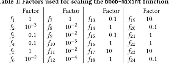
Table 1: Factors used for scaling the bbob-mixint functions.

Factor Factor Factor Factor

f1 1 f7 1 f13 0.1 f19 10 f2 10−3 f8 10−2 f14 1 f20 0.1 f3 0.1 f9 10−2 f15 0.1 f21 1 f4 0.1 f10 10−3 f16 1 f22 1 f5 1 f11 10−2 f17 10 f23 10 f6 10−2 f12 10−4 f18 1 f24 0.1

two values could be interpreted as the ‘middle’ value for variables of even arity, we need to sample among a large set of possible domain middle points. Figure 1 (b) shows the difference between the median f value of 1000 domain middle samples and the f -value of the optimal solution for each problem instance in the bbob-mixint suite prior to scaling. In comparison, Figure 1 (a) shows the difference between the f -value of the domain middle and of the optimal solution for each problem instance for thebbob suite (note that no sampling is required here since it is clear which point is the domain middle in a continuous domain).

Keeping in mind that in COCO the easiest target defaults to 100, we see that for a number ofbbob-mixint functions (f2, f6, f10to

f13and f20), the domain middle rarely (if ever) achieves this target.

On the other hand, for functions such as f17, f19and f23, evaluating

the domain middle already guarantees reaching targets of 10 and less. We also see that the distances for thebbob-mixint suite are very similar to those for thebbob suite, albeit a bit larger in general. Based on these findings and the preliminary algorithm results, we choose to multiply the f -values of the functions with the scaling factors shown in Table 1. This setting is mindful of the connections between some functions, for example, the same scaling factors are used for the original (f8) and rotated (f9) Rosenbrock functions.

Figure 1 (c) shows the result for all (scaled)bbob-mixint problems. Now the f -differences between the domain middle and the optimal solution are more uniform across the problems in the suite.

To summarize, thebbob-mixint suite contains mixed-integer problems constructed by discretizing the continuous problems from thebbob and bbob-largescale suites. Using 24 functions, 6 dimen-sions and 15 instances results in the total of 2160 problem instances.

3.2 The bbob-biobj-mixint Suite

Thebbob-biobj-mixint suite is then constructed by combining two single-objective functions from thebbob-mixint suite (follow-ing the idea of thebbob-biobj and bbob-biobj-ext suites [23]). Instead of making every possible bi-objective combination of two single-objective functions, which would result in a total of 276 (=24·23

2 ) functions, we adopt the selected combinations from the

bbob-biobj-ext suite. This gives us 92 bi-objective functions (see [23] for more details).

Note that, similarly as for thebbob-biobj and bbob-biobj-ext suites, the Pareto sets and fronts of these mixed-integer bi-objective functions are generally unknown as knowing the optima to the single-objective problems only gives us information about the two extreme points of the Pareto set/front. The only exception is the function F1 = (f1, f1), the combination of two sphere functions,

(5)

GECCO ’19, July 13–17, 2019, Prague, Czech Republic Tea Tušar, Dimo Brockhoff, and Nikolaus Hansen 102 ₁₀0 ₁₀2 ₁₀4 ₁₀6 ₁₀8 ₁₀10 f1 f2 f3 f4 f5 f6 f7 f8 f9 f10 f11 f12 f13 f14 f15 f16 f17 f18 f19 f20 f21 f22 f23 f24

Targets reached by

the domain middle (bbob)

dim = 2 dim = 3 dim = 5 dim = 10 dim = 20 dim = 40 102 ₁₀0 ₁₀2 ₁₀4 ₁₀6 ₁₀8 ₁₀10 f1 f2 f3 f4 f5 f6 f7 f8 f9 f10 f11 f12 f13 f14 f15 f16 f17 f18 f19 f20 f21 f22 f23 f24

Estimated targets reached by

the domain middle (bbob-mixint)

dim = 5 dim = 10 dim = 20 dim = 40 dim = 80 dim = 160 10 2 ₁₀0 ₁₀2 ₁₀4 ₁₀6 ₁₀8 ₁₀10 f1 f2 f3 f4 f5 f6 f7 f8 f9 f10 f11 f12 f13 f14 f15 f16 f17 f18 f19 f20 f21 f22 f23 f24

Estimated targets reached by

the domain middle (bbob-mixint)

dim = 5 dim = 10 dim = 20 dim = 40 dim = 80 dim = 160

(a)bbob suite (b)bbob-mixint suite before scaling (c)bbob-mixint suite

Figure 1: Estimation of targets reached by the domain middle (in logarithmic scale). They are computed as the distance between the f -value of the domain middle and the optimal solution for the bbob suite (a), or the median of the distances between the f -values of 1000 domain middle samples and the optimal solution for the bbob-mixint suite before (b) and after (c) scaling. Each circle depicts one problem instance for instances 1–15.

In COCO, assessing the performance of algorithms on a bi-objective problem relies on knowing the hypervolume of its Pareto front. Since we cannot compute it analytically, we resort to esti-mate it by running several different optimization algorithms on the problem for a very large number of evaluations and computing the hypervolume of the resulting non-dominated solutions. This value is then used to set the targets for performance assessment.

4 IMPLEMENTATION IN COCO

Like other benchmark suites available in COCO, thebbob-mixint andbbob-biobj-mixint suites are implemented in C and inter-faced to be used by algorithms in any of the COCO’s supported languages (C/C++, Python, Java and Matlab/Octave). Figure 2 shows how easy it is to interface an optimization algorithm (in this case, the Python implementation of CMA-ES in thepycma package, [8]) with thebbob-mixint suite in Python.

After importing the two Python modules (COCO’s experiments and CMA), thebbob-mixint suite is initialized with default pa-rameters. Then, CMA-ES is run on all problems in the suite. The code snippet shows how to access the relevant information on the problem, such as the number of integer variables and the lower and upper bounds of the region of interest (the total number of variables is inferred by CMA-ES through the initial solution, but can also be obtained throughproblem.dimension).

Thebbob-biobj-mixint suite can be employed in the same way, using a multi-objective algorithm in place of CMA-ES.

i mp o r t cocoex i mp o r t cma

suite = cocoex . Suite ('bbob - mixint ', '', '')

for problem in suite:

cma. fmin2 (problem , problem . initial_solution , 1,

{'bounds ': [problem . lower_bounds ,

problem . upper_bounds],

'integer_variables ': list(range(

problem . number_of_integer_variables )),

'CMA_stds ': ( problem . upper_bounds

- problem . lower_bounds ) / 5},

restarts=9)

Figure 2: Python code to run the CMA-ES algorithm on all problems in the bbob-mixint suite.

5 PROBLEM PROPERTIES

In order to investigate the properties of the proposed test prob-lems, we visualize and discuss, in this section, level sets for the bbob-mixint functions, heat maps for the ellipsoid function, and approximations of the Pareto set and front for the bi-objective double sphere function.

5.1 Level Sets of the bbob-mixint Functions

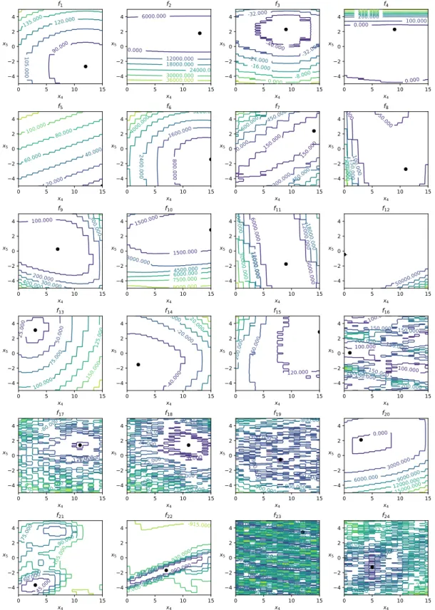
Figure 3 shows the level sets of equal function value of all 24 bbob-mixint functions within the axis-parallel plane through the optimum, spanned by the last two variables (in 5-D). Shown is exemplarily instance 1. Note that in 5-D, only the last variable is

(6)

Mixed-Integer Benchmark Problems for Single- and Bi-Objective Optimization GECCO ’19, July 13–17, 2019, Prague, Czech Republic 0 5 10 15 x4 4 2 0 2 4 x5 90.000 105.000 120.000 135.000 f1 0 5 10 15 x4 4 2 0 2 4 x5 6000.000 6000.000 12000.000 18000.000 24000.000 30000.000 36000.000 f2 0 5 10 15 x4 4 2 0 2 4 x5 -40.000 -32.000 -32.000 -24.000 -16.000 -8.000 0.000 f3 0 5 10 15 x4 4 2 0 2 4 x5 0.000 0.000200.000300.000 100.000 400.000 500.000 600.000 700.000 f4 0 5 10 15 x4 4 2 0 2 4 x5 20.000 40.000 60.000 80.000 100.000 f5 0 5 10 15 x4 4 2 0 2 4 x5 800.000 1600.000 2400.000 3200.000 4000.000 f6 0 5 10 15 x4 4 2 0 2 4 x5 _150.000 150.000 300.000 300.000 450.000 450.000 600.000 f7 0 5 10 15 x4 4 2 0 2 4 x5 50.000 50.000 100.000 150.000 200.000250.000 f8 0 5 10 15 x4 4 2 0 2 4 x5 100.000 200.000 300.000 300.000 400.000 f9 0 5 10 15 x4 4 2 0 2 4 x5 1500.000 1500.000 3000.000 4500.000 6000.000 7500.000 9000.000 f10 0 5 10 15 x4 4 2 0 2 4 x5 6000.000 6000.000 12000.000 12000.000 18000.000 18000.000 24000.000 30000.000 f11 0 5 10 15 x4 4 2 0 2 4 x5 50000.000 f12 0 5 10 15 x4 4 2 0 2 4 x5 25.000 50.000 75.000 100.000 125.000 150.000 f13 0 5 10 15 x4 4 2 0 2 4 x5 -40.000 -20.000 0.000 _20.000 f14 0 5 10 15 x4 4 2 0 2 4 x5 120.000 160.000 200.000 f15 0 5 10 15 x4 4 2 0 2 4 x5 100.000 100.000 100.000 150.000 150.000 150.000 150.000 150.000 200.000 200.000 200.000 f16 0 5 10 15 x4 4 2 0 2 4 x5 -120.000-120.000 -80.000 -40.000 0.000 f17 0 5 10 15 x4 4 2 0 2 4 x5 0.000 25.000 25.00025.000 25.000 25.000 50.000 50.000 75.000 75.000 f18 0 5 10 15 x4 4 2 0 2 4 x5 -900.000 -900.000 -900.000 -800.000 -800.000 -700.000 f19 0 5 10 15 x4 4 2 0 2 4 x5 0.000 3000.000 6000.000 9000.000 12000.000 15000.000 f20 0 5 10 15 x4 4 2 0 2 4 x5 45.000 60.00075.000 75.000 _90.000 105.000 f21 0 5 10 15 x4 4 2 0 2 4 x5 -990.000 -975.000_-975.000 -960.000 -960.000 -945.000 -945.000 -930.000 -930.000 -915.000 f22 0 5 10 15 x4 4 2 0 2 4 x5 180.000 180.000 180.000 180.000 180.000 240.000 240.000_240.000 240.000 240.000 240.000 240.000 240.000 240.000 240.000 240.000 240.000 300.000 300.000300.000 300.000 300.000 300.000 300.000 300.000300.000 300.000 300.000 300.000 300.000300.000 300.000 300.000 300.000300.000 300.000 300.000 f23 0 5 10 15 x4 4 2 0 2 4 x5 _17.500 20.000 20.000 22.500 22.500 f24 bbob-mixint, dimension 5, instance 1

Figure 3: Level sets for the bbob-mixint suite problems of dimension 5, instance 1. The variables chosen for the x and y axis rep-resent the last integer and first continuous variable, respectively. Lighter colors denote higher values. The black dot reprep-resents the optimal solution.

(7)

continuous and the second-to-last one is discrete and has an arity of 16.

At first sight, the level sets show the expected behavior: com-pared to the level sets of the continuous versions from thebbob suite, the level sets for thebbob-mixint functions are piece-wise linear due to the discretization of 80% of the variables.

5.2 A Discretized Unimodal Function Can

Become Multimodal

At closer inspection, however, we see that the high ill-conditioning of some of the problems together with a search space rotation, for example on the ellipsoid function f10, can result in local optima in

the discretized version although the underlying continuous function is unimodal.

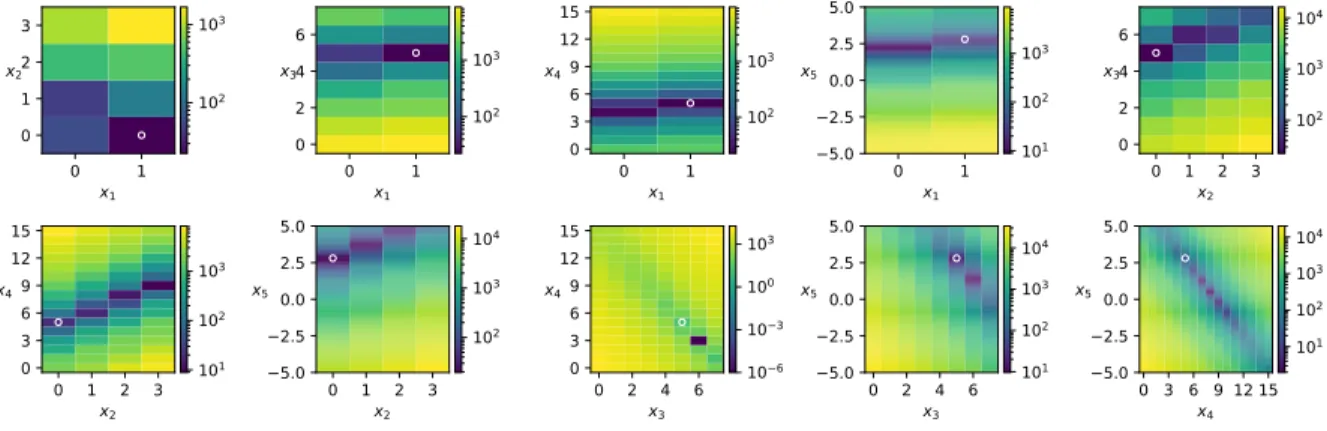
As an example, consider instance 6 in dimension 5 of the el-lipsoid function f10. Figure 4 shows heat maps in all axis-parallel

planes through the search point with x3 = x4 = 5 (white circle)

and all other variable values chosen as the global optimum. This selected search point is obviously not optimal (see the x3-x4plot in

Figure 4), but constitutes a local optimum (i.e. moving to a neigh-boring variable value, function values become worse. Such a local optimum appears if the discretization around the main axis of the high-conditioned ellipsoid is coarse enough such that better search points are only located along the diagonal of the search space but not along the coordinate axes. This is not possible if the original ill-conditioned problem is axis-parallel itself (such as function f2)—

where always one of the neighboring discrete values is improving the objective function.

5.3 Pareto Sets and Fronts for the Discrete

Double Sphere Function

Combining the single-objectivebbob functions to form the func-tions of thebbob-biobj suite already results in complicated and unusual Pareto sets and fronts [2]. Here, we showcase the Pareto sets and fronts of the simplestbbob-biobj-mixint function, the discretized double sphere, in order to see which additional difficul-ties appear when the objective functions of a bi-objective problem are discretized. We chose this function because the underlying con-tinuous problem is the onlybbob-biobj function for which an analytic expression for the Pareto set is known [2].

The Pareto set of the continuous double sphere function is a straight line between the two single-objective optima. In order to visualize the discretized version of it (f1of thebbob-biobj-mixint

suite), we evaluate the search points closest to this (discretized) line. The continuous variables are thereby discretized as well, using 801 points between the two extremes for each reported instance.

Figure 5 shows the resulting non-dominated points for three se-lected instances in dimension 5 and for two instances in dimension 10. The top row presents the projection (in decision space) onto the plane spanned by the two variables with the largest number of distinct values (within the set of non-dominated solutions). The middle row shows the two first principal components of a Princi-pal Component Analysis (PCA) on those non-dominated solutions, while the bottom row displays the corresponding objective vectors in objective space.

We observe the following properties of the function instances: Pareto sets and fronts are discretized and are made up from piece-wise linear parts (in the case of the Pareto set) or piece-piece-wise convex parts (in the case of the Pareto front). The projection of the Pareto set can thereby look connected (in the two rightmost columns) and the Pareto front, globally, is not convex everywhere (see for example the middle part of the Pareto front in Figure 5 (b)). The number of non-connected Pareto set and Pareto front parts differs widely from instance to instance. This seems to depend on the number of distinct variable values among the non-dominated solutions in the considered solution sets and thus indirectly by the placement of the two single-objective optima with respect to the discretization grid, which is exactly the difference among instances of the double sphere function.

6 EXAMPLE ALGORITHM PERFORMANCE

In this section we investigate the newly proposedbbob-mixint suite from an algorithm standpoint: how difficult is it to solve thebbob-mixint problems in terms of the number of function evaluations to reach certain target difficulties? To this end, we implemented thebbob-mixint functions in the COCO platform, run four algorithms on them and report and discuss the results here in terms of empirical cumulative distribution functions of the recorded runtimes.

Algorithm Details. Overall, we chose four algorithms to run on thebbob-mixint suite—a selection which contains algorithms from various domains but which is also not exhaustive or in any way representative of the entire set of available algorithms for mixed-integer optimization. The main focus here is still the introduction of a new test suite and not the benchmarking of a large portion of the existing algorithms.

The four selected algorithms are

• Random Search as a baseline, sampling each variable uni-formly at random within their bounds (i.e., from [-5,5] for the continuous variables, from 0 to the maximum value for the integer ones),

• Differential Evolution (DE) [21] with the strategy ’rand/1/bin’ and population size 10 · (4+ ⌊3 log(n)⌋), implemented in the scipy Python module [12], handling the problems as if they were continuous and bounded by their region of interest, • a CMA-ES variant for mixed-integer optimization [7] as

showcased in Figure 2 (but without restarts) with boundary handling and a variable-wise initial step size that is chosen relative to the difference between the smallest and largest value, and finally

• TPE (Tree-structured Parzen Estimator, [1]), a common al-gorithm for hyperparameter tuning, as implemented in the Python modulehyperopt.

For TPE, the discrete variables have been represented with a uniform distribution on their discrete values and for the continuous variables, we used a normal distribution with mean 0 and standard deviation 2. The experiments were run for a budget of 104n for Random Search, DE, and CMA-ES and for a budget of 50n for TPE (due its long internal runtime). If not mentioned otherwise, we use the default settings for each algorithm.

(8)

Mixed-Integer Benchmark Problems for Single- and Bi-Objective Optimization GECCO ’19, July 13–17, 2019, Prague, Czech Republic 0 1 x1 0 1 2 3 x2 0 1 x1 0 2 4 6 x3 0 1 x1 0 3 6 9 12 15 x4 0 1 x1 5.0 2.5 0.0 2.5 5.0 x5 0 1 2 3 x2 0 2 4 6 x3 0 1 2 3 x2 0 3 6 9 12 15 x4 0 1 2 3 x2 5.0 2.5 0.0 2.5 5.0 x5 0 2 4 6 x3 0 3 6 9 12 15 x4 0 2 4 6 x3 5.0 2.5 0.0 2.5 5.0 x5 0 3 6 9 12 15 x4 5.0 2.5 0.0 2.5 5.0 x5 102 103 102 103 102 103 101 102 103 102 103 104 101 102 103 102 103 104 106 103 100 103 101 102 103 104 101 102 103 104

Figure 4: Heat maps of the bbob-mixint rotated ellipsoid function (f10) in dimension 5, instance 6. The white circle indicates

the solution at (x₁opt,x₂opt,5,5,x₅opt) which is a local optimum.

(a) Dim 5, instance 1 (b) Dim 5, instance 7 (c) Dim 5, instance 10 (d) Dim 10, instance 8 (e) Dim 10, instance 11 Figure 5: Optimal solutions to the bbob-mixint suite double sphere problems (function F1) of different dimensions and

in-stances depicted in the decision (top), PCA (middle) and objective (bottom) spaces. The decision space plots are projections to the 2-D space of the two variables that have the highest number of distinct values. The PCA plots show the projection using the first two principal components. In addition to showing the Pareto fronts, the objective space plots contain information of the number of visualized solutions (equal for all three plots of the same problem).

Display Settings. For the displayed algorithm performance, we fall back on the empirical cumulative distribution plots (ECDF) of the recorded runtimes that the COCO framework provides by de-fault for new test suites. Because of the scaling of thebbob-mixint

functions (see Section 3.1.3), we can keep the standard target diffi-culties of 51 values, uniformly chosen on a logscale between 100 and 10−8. All experiments have been run on instances 1–15.

(9)

0 2 4 6

log10(# f-evals / dimension) 0.0 0.2 0.4 0.6 0.8 1.0

Fraction of function,target pairs hyperopt-RS-bbob-m DE-bbob-m CMA-bbob-bbob-mixint f1-f24, 5-D 51 targets: 100..1e-08 15 instances v2.2.1.1116 0 2 4 6

Fraction of function,target pairs RS-bbob-m hyperopt- CMA-bbob-DE-bbob-m bbob-mixint f1-f24, 10-D 51 targets: 100..1e-08 15 instances v2.2.1.1116 0 2 4 6

Fraction of function,target pairs hyperopt-RS-bbob-m DE-bbob-m CMA-bbob-bbob-mixint f1-f24, 20-D 51 targets: 100..1e-08 15 instances v2.2.1.1116 0 2 4 6

Fraction of function,target pairs hyperopt-RS-bbob-m CMA-bbob-DE-bbob-m bbob-mixint f1-f24, 40-D 51 targets: 100..1e-08 15 instances v2.2.1.1116 0 2 4 6

Fraction of function,target pairs RS-bbob-m hyperopt-DE-bbob-m CMA-bbob-bbob-mixint f1, 5-D 51 targets: 100..1e-08 15 instances v2.2.1.1116 1 Sphere 0 2 4 6

Fraction of function,target pairs hyperopt-RS-bbob-m CMA-bbob-DE-bbob-m bbob-mixint f2, 5-D 51 targets: 100..1e-08 15 instances v2.2.1.1116 2 Ellipsoid separable 0 2 4 6

Fraction of function,target pairs hyperopt-RS-bbob-m DE-bbob-m CMA-bbob-bbob-mixint f14, 5-D 51 targets: 100..1e-08 15 instances v2.2.1.1116 14 Sum of different powers

0 2 4 6

Fraction of function,target pairs RS-bbob-m DE-bbob-m CMA-bbob- hyperopt-bbob-mixint f21, 5-D 51 targets: 100..1e-08 15 instances v2.2.1.1116 21 Gallagher 101 peaks 0 2 4 6

Fraction of function,target pairs RS-bbob-m hyperopt- CMA-bbob-DE-bbob-m bbob-mixint f1, 20-D 51 targets: 100..1e-08 15 instances v2.2.1.1116 1 Sphere 0 2 4 6

Fraction of function,target pairs RS-bbob-m hyperopt- CMA-bbob-DE-bbob-m bbob-mixint f2, 20-D 51 targets: 100..1e-08 15 instances v2.2.1.1116 2 Ellipsoid separable 0 2 4 6

Fraction of function,target pairs RS-bbob-m hyperopt- CMA-bbob-DE-bbob-m bbob-mixint f14, 20-D 51 targets: 100..1e-08 15 instances v2.2.1.1116 14 Sum of different powers

0 2 4 6

Fraction of function,target pairs hyperopt-RS-bbob-m DE-bbob-m CMA-bbob-bbob-mixint f21, 20-D 51 targets: 100..1e-08 15 instances v2.2.1.1116 21 Gallagher 101 peaks

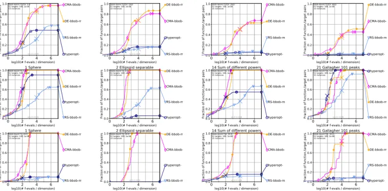
Figure 6: Empirical cumulative distribution of simulated runtimes over 51 targets for four selected mixed-integer algorithms. The first row shows the results aggregated over all 24 bbob-mixint functions in dimensions 5, 10, 20, and 40 (from left to right). The second (in dimension 5) and third row (in dimension 20) shows results for four selected bbob-mixint functions.

Algorithm Performances. The ECDFs for the four selected algo-rithms, aggregated over all 24bbob-mixint functions, can be found in the top row of Figure 6 for dimensions 5, 10, 20, and 40. Selected single-function ECDFs are shown in the middle row for dimension 5 and in the bottom row for dimension 20. We see that:

•Over all bbob-mixint problems, the algorithms perform worse with increasing dimension.

•Random Search and TPE (with its small budget of 50n func-tion evaluafunc-tions) are effected the most such that only very few targets are reached in dimension 40. For the functions with low or moderate conditioning (f6–f9), not a single

tar-get ≤ 100 is reached in dimensions 40 and higher (plot not shown here). DE and CMA-ES, on the contrary, still solve about 35–40% of the targets up to their budget in dimension 40. These trends continue in higher dimensions (not shown). •TPE is highly negatively affected by ill-conditioned func-tions. When we compare the results on the sphere function and axis-parallel ellipsoid in dimension 5, we observe that the fixed sample distribution of TPE is relatively effective for the isotropic sphere function (following the performance of DE and CMA-ES up within its assigned budget), but not any-more for the squeezed level sets of the highly ill-conditioned ellipsoid function (where the performance of TPE is worse than the one for Random Search in dimension 5).

7 CONCLUSIONS

In this paper we have introduced two mixed-integer benchmark testbeds with scalable functions between dimensions 5 and 160.

Our testbeds are based on two benchmark suites available in the COCO benchmarking platform and have been implemented within the platform asbbob-mixint and bbob-biobj-mixint suites.

We investigated properties of the functions of the new suites and found that discretization has a remarkable impact on the function properties in some cases. Taking a closer look at some unimodal functions of the single-objectivebbob-mixint suite, we found that discretization of non-separable ill-conditioned convex-quadratic functions is likely to introduce local optima in the originally uni-modal problem. We also can understand the mechanism: given a direction of improvement is diagonal, we have to change several co-ordinates to get to the next better setting. We conjecture that these new discretized functions are much harder problems to optimize than their continuous counterparts.

Investigating the Pareto fronts and sets of instances of the dis-cretized double sphere function, we found a rich variety of discon-nected shapes already for this supposedly simplest of all bi-objective function, standing in stark contrast to the simple Pareto front/set of its continuous version. Hence it will take some effort to identify the Pareto fronts of the new bi-objective functions to make them available for comparative benchmarking.

ACKNOWLEDGMENTS

The first author acknowledges the financial support from the Slove-nian Research Agency (project No. Z2-8177). This work was sup-ported by a public grant as part of the Investissement d’avenir project, reference ANR-11-LABX-0056-LMH, LabEx LMH, in a joint call with Gaspard Monge Program for optimization, operations research and their interactions with data sciences.

(10)

Mixed-Integer Benchmark Problems for Single- and Bi-Objective Optimization GECCO ’19, July 13–17, 2019, Prague, Czech Republic

REFERENCES

[1] J. Bergstra, R. Bardenet, Y. Bengio, and B. Kegl. 2011. Algorithms for hyper-parameter optimization. In Proceedings of the Annual Conference on Neural Infor-mation Processing Systems (NIPS 2011). 2546–2554.

[2] D. Brockhoff, T. Tušar, A. Auger, and N. Hansen. 2019. Using well-understood single-objective functions in multiobjective black-box optimization test suites. ArXiv e-prints arXiv:1604.00359v3 (2019).

[3] D. Brockhoff, T. Tušar, D. Tušar, T. Wagner, N. Hansen, and A. Auger. 2016. Biobjective performance assessment with the COCO platform. ArXiv e-prints arXiv:1605.01746 (2016).

[4] M. R. Bussieck, A. S. Drud, and A. Meeraus. 2003. MINLPLib – A collection of test models for mixed-integer nonlinear programming. INFORMS Journal on Computing 15, 1 (2003), 114–119.

[5] K. Deep, K. P. Singh, M. L. Kansal, and C. Mohan. 2009. A real coded genetic algorithm for solving integer and mixed integer optimization problems. Appl. Math. Comput. 212, 2 (2009), 505–518.

[6] S. Finck, N. Hansen, R. Ros, and A. Auger. 2009. Real-parameter black-box opti-mization benchmarking 2009: Presentation of the noiseless functions. Technical Report 2009/20. Research Center PPE, Austria. http://coco.lri.fr/downloads/ download15.03/bbobdocfunctions.pdf Updated February 2010.

[7] N. Hansen. 2011. A CMA-ES for mixed-integer nonlinear optimization. Technical Report RR-7751. Inria, France. https://hal.inria.fr/inria-00629689/en/ [8] N. Hansen, Y. Akimoto, and P. Baudis. 2019. CMA-ES/pycma on Github. Zenodo.

(Feb. 2019). https://doi.org/10.5281/zenodo.2559634

[9] N. Hansen, A Auger, D. Brockhoff, D. Tušar, and T. Tušar. 2016. COCO: Perfor-mance assessment. ArXiv e-prints arXiv:1605.03560 (2016).

[10] N. Hansen, A. Auger, O. Mersmann, T. Tušar, and D. Brockhoff. 2016. COCO: A platform for comparing continuous optimizers in a black-box setting. ArXiv e-prints arXiv:1603.08785 (2016).

[11] F. Hutter, M. López-Ibánez, C. Fawcett, M. Lindauer, H. H. Hoos, K. Leyton-Brown, and T. Stützle. 2014. AClib: A benchmark library for algorithm configuration. In Proceedings of the International Conference on Learning and Intelligent Optimiza-tion (LION 8) (Lecture Notes in Computer Science), Vol. 8426. Springer, 36–40. [12] E. Jones, T. Oliphant, P. Peterson, et al. 2001–. SciPy: Open source scientific tools

for Python. (2001–). http://www.scipy.org/ [Online; accessed 5. 2. 2019].

[13] S. A. Kauffman. 1993. The Origins of Order: Self-Organization and Selection in Evolution. OUP USA.

[14] R. Li, M. T. M. Emmerich, J. Eggermont, T. Bäck, M. Schütz, J. Dijkstra, and J. H. C. Reiber. 2013. Mixed integer evolution strategies for parameter optimization. Evolutionary computation 21, 1 (2013), 29–64.

[15] R. Li, M. T. M. Emmerich, J. Eggermont, E. G. P. Bovenkamp, T. Bäck, J. Dijkstra, and J. H. C. Reiber. 2006. Mixed-integer NK landscapes. In Proceedings of the International Conference on Parallel Problem Solving from Nature (PPSN IX) (Lecture Notes in Computer Science), Vol. 4193. Springer, 42–51.

[16] T. Liao, K. Socha, M. A. M. de Oca, T. Stützle, and M. Dorigo. 2014. Ant colony optimization for mixed-variable optimization problems. IEEE Transactions on Evolutionary Computation 18, 4 (2014), 503–518.

[17] T. W. Liao. 2010. Two hybrid differential evolution algorithms for engineering design optimization. Applied Soft Computing 10, 4 (2010), 1188–1199. [18] K. McClymont and E. Keedwell. 2011. Benchmark multi-objective optimisation

test problems with mixed encodings. In Proceedings of the IEEE Congress on Evolutionary Computation (CEC 2011). IEEE, 2131–2138.

[19] J. J. Moré and S. M. Wild. 2009. Benchmarking derivative-free optimization algorithms. SIAM Journal on Optimization 20, 1 (2009), 172–191.

[20] J. Müller. 2016. MISO: Mixed-integer surrogate optimization framework. Opti-mization and Engineering 17, 1 (2016), 177–203.

[21] R. Storn and K. V. Price. 1997. Differential evolution – A simple and efficient heuristic for global optimization over continuous spaces. Journal of Global Optimization 11, 4 (1997), 341–359.

[22] P. N. Suganthan, N. Hansen, J. J. Liang, K. Deb, Y.-P. Chen, A. Auger, and S. Tiwari. 2005. Problem definitions and evaluation criteria for the CEC 2005 special session on real-parameter optimization. KanGAL report 2005005. IIT Kanpur, India. [23] T. Tušar, D. Brockhoff, N. Hansen, and A. Auger. 2016. COCO: The bi-objective

black-box optimization benchmarking (bbob-biobj) test suite. ArXiv e-prints arXiv:1604.00359 (2016).

[24] K. Varelas, A. Auger, D. Brockhoff, N. Hansen, O. A. ElHara, Y. Semet, R. Kassab, and F. Barbaresco. 2018. A comparative study of large-scale variants of CMA-ES. In Proceedings of the International Conference on Parallel Problem Solving from Nature (PPSN XV) (Lecture Notes in Computer Science), Vol. 11101. Springer, 3–15.