• Aucun résultat trouvé

Safe screening for sparse regression with the Kullback-Leibler divergence

N/A
N/A
Protected

Academic year: 2021

Partager "Safe screening for sparse regression with the Kullback-Leibler divergence"

Copied!
6
0
0

Texte intégral

(1)

HAL Id: hal-03147345

https://hal.archives-ouvertes.fr/hal-03147345v2

Submitted on 21 Apr 2021

HAL is a multi-disciplinary open access

archive for the deposit and dissemination of

sci-entific research documents, whether they are

pub-lished or not. The documents may come from

teaching and research institutions in France or

abroad, or from public or private research centers.

L’archive ouverte pluridisciplinaire HAL, est

destinée au dépôt et à la diffusion de documents

scientifiques de niveau recherche, publiés ou non,

émanant des établissements d’enseignement et de

recherche français ou étrangers, des laboratoires

publics ou privés.

Safe screening for sparse regression with the

Kullback-Leibler divergence

Cassio Dantas, Emmanuel Soubies, Cédric Févotte

To cite this version:

Cassio Dantas, Emmanuel Soubies, Cédric Févotte. Safe screening for sparse regression with the

Kullback-Leibler divergence. IEEE International Conference on Acoustics, Speech and Signal

Pro-cessing (ICASSP), Jun 2021, Toronto (virtual), Canada. �hal-03147345v2�

(2)

SAFE SCREENING FOR SPARSE REGRESSION WITH

THE KULLBACK-LEIBLER DIVERGENCE

C´assio F. Dantas, Emmanuel Soubies, C´edric F´evotte

IRIT, Universit´e de Toulouse, CNRS, Toulouse, France

ABSTRACT

Safe screening rules are powerful tools to accelerate iterative solvers in sparse regression problems. They allow early iden-tification of inactive coordinates (i.e., those not belonging to the support of the solution) which can thus be screened out in the course of iterations. In this paper, we extend the GAP Safe screening rule to the `1-regularized Kullback-Leibler

diver-gence which does not fulfil the regularity assumptions made in previous works. The proposed approach is experimentally validated on synthetic and real count data sets.

Index Terms— Safe screening, KL divergence, sparsity. 1. INTRODUCTION

The Poisson observation model has been used in a variety of applications where data correspond to a series of discrete events with inherently noisy measurements. Examples in-clude: nuclear medical imaging (e.g., Positron emission to-mography [1]), astronomy [2] and traffic analysis [3]. The lin-ear case can be written as: y ∼ Poisson(Ax), where y ∈ Rm+

is the observation vector, x ∈ Rn+ is the signal of interest,

and A ∈ Rm×n+ is the measurement matrix. Poisson

intensi-ties are naturally non-negative (thus the natural non-negativity constraints).

In this context, recovering the signal of interest x from the observations y amounts to the resolution of a linear in-verse problem. The resulting problem is usually ill-posed as m < n (number of observations smaller than the number of unknowns) which motivates the introduction of a regulariza-tion term based on some prior knowledge on the signal x. In this paper, we are interested in sparsity prior which can be achieved via a `1-norm regularization. This leads to the

fol-lowing optimization problem: x?∈ argmin

x∈Rn +

Pλ(x) := DKL(y | Ax) + λkxk1 (1)

where Pλ(x) denotes the primal objective function,

parame-ter λ > 0 controls the sparsity level of the solution, and the data-fidelity term is the generalized Kullback-Leibler (KL)

This work is supported by the European Research Council (ERC FACTORY-CoG-6681839). Code is available at https://github.com/ cassiofragadantas.

divergence [4], which also corresponds to the Poisson neg-ative log-likelihood up to irrelevant terms [5, 6]:

DKL(y | z) = m X i=1 yilog  y i zi+   − yi+ (zi+ ). (2)

The smoothing constant  ≥ 0 allows to avoid singularities around zi= 0 and is common practice, see, e.g., [7].

Several algorithms have been proposed in the literature for tackling problem (1) [4, 7, 8, 9]. In this paper, we propose a variable elimination technique called safe screening that can accelerate most of the existing solvers.

Safe screening techniques were originally proposed for the Lasso problem [10], but have recently been extended to a wide variety of sparse-regularized problems [11, 12, 13]. Such techniques allow to identify, before and while solving the problem, coordinates which will not be part of the so-lution support. Doing so might significantly accelerate the problem’s resolution. As soon as a coordinate j is identified as inactive, the corresponding column of the dictionary matrix ajcan be removed once and for all. In such approaches, there

is no risk of false identification, thus the “safe” denomination. In this paper, we extend an existing screening tech-nique [12] to the regularized Kullback-Leibler problem (1). Even though the approach in [12] was proposed within a generalized linear model framework, it cannot be directly applied to our problem of interest, since the Kullback-Leibler function does not fulfill the regularity hypothesis in [12].

In Section 2, we go through the main technical ingredi-ents on deriving safe screening rules for problem (1). Then, the proposed algorithm is described in Section 3 and experi-mental results are given in Section 4.

Notations [n] = {1, . . . , n} is the set of n first integers and 1 is a vector of ones (with size inferred from context). θI ∈

R|I| denotes the restriction of θ ∈ Rm to its components indexed by the elements of I ⊆ [m]. I{ denotes the com-plement of set I. Given two vectors z ∈ Rmand y ∈ Rm, y/z is the entry-wise division. We denote ∇DKL(y | z) =

∇zDKL(y | z) the gradient w.r.t. the second variable z ∈ Rm+

(3)

2. SAFE SCREENING FOR THE KL-`1PROBLEM

2.1. The Dual Problem

Theorem 1. The dual formulation of the optimization prob-lem defined in(1) is given by:

θ?= argmax θ∈FA Dλ(θ) := m X i=1 yilog(1 + λθi) − λθi, (3)

whereFA = {θ ∈ Rm| λθ ≥ −1, ATθ ≤ 1} is the dual

feasible set and“ ≤ ” is defined component-wisely. More-over, first-order optimality conditions for a pair of solutions (x?, θ?) are given by:

λθ?= y Ax?+ − 1 (4) aTjθ?=  1, if x? j > 0, % ≤ 1, if x? j = 0. (5) Proof. The dual function Dλ(θ) is given by the Fenchel

conjugate of the data-fidelity term DKL[12, 14]. The

con-straint set is given by the Fenchel conjugate of Ω(x) = kxk1+ 1Rm+(x), which is calculated in [13] for the

nonnega-tive Lasso. For compactness, we integrate to the feasible set the domain of the dual function, given by dom(Dλ) = {θ ∈

Rm| θ ≥ −1/λ}.

Optimality conditions (4) and (5) are given by [12]: λθ?= −∇DKL(y | Ax?)

ATθ?∈ ∂kxk1+ ∂1Rm+(x)

Calculation details for the latter equation are given in [13]. Finally, it is worth mentioning that, even for  = 0, (4) is well-defined as [Ax?]i= 0 =⇒ yi= 0, in which case we use the

convention that 0/0 = 0. Indeed, when  = 0, if yi 6= 0 and

[Ax]i= 0 for any i ∈ [m], then DKL(y | Ax) = +∞ which

cannot be optimal and, hence, yi 6= 0 =⇒ [Ax?]i 6= 0 as

desired.

A direct consequence of Theorem 1 is that, given the dual solution θ?,

aTjθ ?

< 1 =⇒ x?j = 0, (6)

for any primal solution x?. In other words, the support of primal solutions x?is characterized by the knowledge of the dual solution. The promise of safe screening is then to ex-ploit this property in order to reduce the size of the primal problem (and accelerate its resolution) by screening out the coordinates that are inactive (x?

j = 0).

2.2. Safe Sphere

Because the dual solution θ? is not known in advance, the condition (6) cannot be used in practice. However, we can derive a more restrictive—yet practical—sufficient condition for eliminating coordinates of the primal problem.

Proposition 1 (KL-`1Safe Screening Rule). Let I = {i ∈

[m] : yi= 0} and S = {θ ∈ Rm| θI = −1/λ}. Let θ ∈ S

andr > 0 be such that θ?∈ B(θ, r). Then,

aTjθ + rk[aj]I{k2< 1 =⇒ x?j = 0. (7)

Proof. First of all, one can see from (4) that the dual solu-tion takes the value θ?

i = −1/λ for all coordinates i ∈ I.

Hence, by the definition of S, we have θ? ∈ S and thus θ?∈ B(θ, r) ∩ S. It follows from (5) that

sup ξ∈B(θ,r)∩S aTjξ < 1 =⇒ aTjθ?< 1 =⇒ x?j = 0. Finally, we have sup ξ∈B(θ,r)∩S aTjξ = aTjθ + r sup u∈B(0,1),uI=0 aTju = aTjθ + rk[aj]I{k2

which completes the proof.

Hence, if one can find a ball B(θ, r) containing θ? (we say that B(θ, r) is a safe region), Proposition 1 allows to safely identify inactive variables of x?. This is possible when

the dual function is α-strongly concave [12]. Indeed, given a primal-dual feasible pair (x, θ) ∈ Rn+× FA, the authors

in [12] have shown that B(θ, r) with r =p2 Gapλ(x, θ)/α, where Gapλ(x, θ) := Pλ(x) − Dλ(θ) denotes the duality

gap, is a safe region (GAP Safe Sphere). Unfortunately, for the KL divergence, the dual objective function Dλin (3) is not

globally strongly concave. However, Dλ is locally strongly

concave and we shall show that this is sufficient to derive a safe region B(θ, r).

Theorem 2 (KL-`1 GAP Safe Sphere). Let I and S be

de-fined as in Proposition 1.Let(x, θ) ∈ Rn+× (FA∩ S) be

a primal-dual feasible pair, and assume that rank(A) =

min(m, n). Then, for

r = r 2 Gapλ(x, θ) ¯ α (8) ¯ α = λ2min i∈I{ yi (1 + max(kAk1, λ)ka†ik1)2 , (9)

we haveθ? ∈ B(θ, r) (i.e., B(θ, r) is a safe region). In (9) a†i denotes thei-th column of A†∈ Rn×m, the right

pseudo-inverse ofA such that AA†= Im, andkAk1is the maximum

absolute column sum of the matrixA.

Proof. Because by definition and assumption we have both θ? ∈ FA∩ S and θ ∈ FA∩ S, it is sufficient to have Dλ

¯

α-strongly concave on FA ∩ S to complete the proof by

following the same steps as in [12][Theorem 2]. Hence,

let us show that Dλ is ¯α-strongly concave in FA ∩ S.

(4)

by ∇2Dλ(θ) = Diag h −λ2 yi (1+λθi)2 i i∈[m]  . The i-th

eigenvalue σi (i.e., the i-th diagonal entry) depends only on

the i-th coordinate θiand may tend to zero as |θi| → +∞.

However, when we restrict ourselves to the dual feasible set, FA = {θ | ATθ ≤ 1, θ ≥ −1/λ}, |θi| can be bounded as

follows (provided that rank(A) = min(m, n)) |θi| = |(AA†)Tθ  i| = |ha † i, A Tθi| ≤ ka† ik1kATθk∞.

The definition of FAimplies that −AT1/λ ≤ ATθ ≤ 1, or

equivalently kATθk

∞≤ max (kAk1/λ, 1) . Therefore:

(1 + λθi)2≤ (1 + max(kAk1, λ)ka†ik1)2

which leads to a bound on the i-th eigenvalue. Finally, by re-stricting ourselves to the set S = {θ ∈ Rm| θI = −1/λ},

all coordinates i ∈ I are fixed and the corresponding eigen-values can be ignored. Hence,

max i∈I{ σi≤ −λ2min i∈I{ yi (1 + max(kAk1, λ)ka†ik1)2 := − ¯α

completes the proof.

Remark 1. To derive the safe sphere in Theorem 2, we ex-ploit the local strong-concavity property of the dual function Dλ over FA ∩ S. The restriction to the set S ⊆ Rm−|I|

is essential to obtain this strong-concavity property asDλis

not strongly-concave onFA. More generally, this result is an

example of how prior knowledge on the dual solution can be leveraged to improve screening strategies.

3. PROPOSED ALGORITHM

Equipped with the screening tools derived in Section 2, we can deploy the so-called dynamic screening approach [11] to accelerate iterative solvers for problem (1). The idea is to per-form screening tests repeatedly over the iterations of the un-derlying solver. As the algorithm converges, smaller safe re-gions can be defined, leading to a growing number of screened coordinates. This strategy is described in Algorithm 1 for a generic iterative solver for (1) (see Section 3.1) whose update step is denoted

{x, η} ← PrimalUpdate(x, A, y, λ, η). (10)

In (10), x stands for the current estimate of the primal vari-able and η is a list of auxiliary varivari-ables (e.g., the gradient step-size, and possibly a few previous primal estimates). The stopping condition is given by a threshold gapon the duality

gap. Finally, in order to exploit the safe region derived in The-orem 2 for screening, it is needed to compute a dual feasible point θ ∈ FA∩ S from the current primal estimate x (line 5

in Algorithm 1). This is discussed in Section 3.2.

For simplicity, in Algorithm 1 screening is performed af-ter every iaf-teration of the solver, but it can actually be formed at any chosen moment. For instance, it can be per-formed on regular intervals between a certain number of iter-ations of the solver. Finally, note the nested characteristic of the preserved set (line 7) as the screened coordinates are no longer tested on the ensuing iterations.

Algorithm 1 ˆx = ScreeningSolverKL(A, y, λ, x, εgap)

1: Initialize: A = [n], η according to the solver

2: repeat

3: {xA, η} ← PrimalUpdate(xA, AA, y, λ, η)

4: —– Dynamic Screening —–

5: θ ← Θ (x) . Dual update (Proposition 2)

6: r ← q

2 Gapλ(x,θ) ¯

α . Safe radius (Theorem 2)

7: A ← {j ∈ A | aTjθ + rk[aj]Ik2≥ 1}

8: xA{← 0

9: until Gapλ(x, θ) < εgap

As screening progressively reduces the number of co-ordinates in play, the solver iteration cost decreases pro-portionally. The screening test itself does not represent a considerable overhead since it reuses the calculations

already performed by the solver update. For instance,

Θ (x) given in Proposition 2 requires the computation of ρ(x) = ∇DKL(y | Ax) and ATρ(x), which are calculated

by basically any first-order solver. Similarly, the duality gap can be reused as the stopping criterion.

3.1. Primal Update

Basically any standard iterative solver for problem (1) can be used in Algorithm 1. In the present paper, we focus on the following ones:

1. Multiplicative update (MU) [1, 2, 4, 15] 2. Proximal gradient descent (SPIRAL [7]) 3. Coordinate descent (CoD) [8] (or [16]) 3.2. Dual Update

The sphere center in Theorem 2 is given by a dual feasible point θ ∈ FA∩ S. Apart from primal-dual approaches such

as [17, 14], most popular solvers for problem (1) only provide a primal solution estimate x at each iteration [4, 7, 8]. Hence, in this scenario, one needs to compute θ ∈ FA∩ S from x.

This can be achieved at a low computational cost following Proposition 2 which is inspired from [11, 12].

Proposition 2. Let x ∈ Rn

+be a primal feasible point and set

ρ(x) = y/(Ax + ) − 1. Then Θ : Rn +→ Rm+ defined by [Θ(x)]i= ( [ρ(x)] i λ max(1,max(ATρ(x)/λ)) if i ∈ I{ −1 λ if i ∈ I (11)

(5)

is such thatΘ(x) ∈ FA∩ S. Moreover, we have Θ(x) → θ?

asx → x?.

Proof. Clearly, by definition of Θ, we have Θ(x) ∈ S. It remains to show that Θ(x) ∈ FA. Because A ∈ Rm×n+ ,

x ∈ Rn+, and y ∈ Rm+, we have that ρ/λ ≥ −1/λ.

Combin-ing this with max 1, max ATρ(x)/λ ≥ 1 and (11), we

obtain that max(1,max(Aρ(x)/λTρ(x)/λ)) ≥ Θ(x) ≥ −1/λ.

Multi-plying the left and right hand side of the first inequality by AT, we obtain ATΘ(x) ≤ 1 which shows that Θ(x) ∈ F

A.

Moreover, by continuity of ρ we obtain ρ(x) →

x→x?ρ(x

?) = (4)λθ

?

which, together with (5) and (11) proves that Θ(x) → θ?as x → x?.

4. EXPERIMENTS

In this section, we evaluate the performance of Algorithm 1 coupled with the three standard solvers listed in Section 3.1 for the resolution of (1) with  = 10−6. Note that values for the hyperparameter λ are reported relatively to λmax =

max AT(y − ) / (the bound above which x?= 0).

4.1. A Synthetic Toy Example

We generate synthetic data that follow the Poisson noise model y = Poisson(Ax) with dimensions m = 10, n = 20. The entries of A are drawn i.i.d. with half-normal distribution (i.e., entry aij = |bij| with bij ∼ N (0, 1)), the columns aj

are then rescaled to unit-norm and x is a 2-sparse vector with uniformly-distributed nonzero entries.

Figure 1 illustrates a typical behavior of a MU solver paired with the proposed screening strategy. Screening intro-duces actual zeroes in the solution estimate, something that would not be possible with a regular MU solver, which can only shrink the coordinates without ever making them zero. 4.2. Real Datasets

We now consider real count datasets: 20-Newsgroups [18], NIPS papers [19] (word counts) and TasteProfile [20] (song listening counts). The observation vector y is a randomly se-lected column of the count data matrix and A is formed by the remaining data, akin to archetypal analysis.

Figure 2 shows an instance of the CoD solver’s conver-gence over time with and without screening. Note that screen-ing progressively reduces the iteration cost which leads to a considerable acceleration in convergence time.

Finally, Table 1 summarizes speedup results for the tested datasets with the three considered solvers in different reg-ularization regimes and for different convergence criteria. Speedups from 1.5 to 8 times are observed, with larger gains obtained for smaller convergence tolerances (εgap).

0 50 100 150 Iteration number 10-15 10-10 10-5 Coordinate value 0 50 100 150 Iteration number 5 10 15 20 Coordinate x j 0 50 100 150 Iteration number 0 10 20 Total screened

Fig. 1: Screening behavior with MU solver. Problem param-eters: m = 10, n = 20, λ = 10−3λmax. Left: each line is a

coordinate xj, the line stops when the coordinate is screened.

Top: rows are coordinates which turn white when screened. Bottom: Total number of screened coordinates per iteration.

0 0.1 0.2 0.3 0.4 0.5 Time [s] 10-10 10-5 100 Duality gap CoD CoD + screening

Fig. 2: Convergence of CoD solver in CPU time. 20 News-groups data, λ = 10−2λmax.

5. CONCLUSION

A dynamic screening approach has been proposed to ac-celerate existing iterative solvers for the sparse-regularized Kullback-Leibler minimization problem. In particular, we have shown that the local strong-concavity of the associated dual function is sufficient to derive a safe screening rule. This idea could be extended for other data-fidelity terms where the dual objective function is not globally strongly concave, pushing the limits of existing safe screening rules. The pro-posed approach provided consistent speedups in a wide range of tested scenarios. λ/λmax 10−1 10−3 εgap 10−5 10−7 10−5 10−7 SPIRAL 1.44 1.59 1.60 1.78 20 Newsgr. CoD 2.44 3.42 2.46 3.22 MU 4.80 7.72 4.49 7.28 SPIRAL 2.77 3.21 2.26 2.53

NIPS papers CoD 4.19 5.35 4.12 5.06

MU 6.71 8.88 5.74 7.31

SPIRAL 2.54 3.00 2.82 3.21

TasteProfile CoD 1.75 2.20 2.44 4.22

MU 2.81 4.11 2.94 4.35

(6)

6. REFERENCES

[1] W. H. Richardson, “Bayesian-based iterative method of image restoration,” Journal of the Optical Society of America, vol. 62, pp. 55–59, 1972.

[2] L. B. Lucy, “An iterative technique for the rectification of observed distributions,” Astronomical Journal, vol. 79, pp. 745–754, 1974.

[3] V. S. Frost and B. Melamed, “Traffic modeling for

telecommunications networks,” IEEE Communications Magazine, vol. 32, no. 3, pp. 70–81, 1994.

[4] Daniel D. Lee and H. Sebastian Seung, “Algorithms for non-negative matrix factorization,” in Advances in Neural Information Processing Systems (NeurIPS). MIT Press, 2001.

[5] D. M. Titterington, “On the iterative image space re-construction algorthm for ECT,” IEEE Transactions on Medical Imaging, vol. 6, no. 1, pp. 52–56, 1987. [6] N. Pustelnik, C. Chaux, and J. Pesquet, “Hybrid

regu-larization for data restoration in the presence of Poisson noise,” in Proc. European Signal Processing Conference (EUSIPCO), 2009.

[7] Z. T. Harmany, R. F. Marcia, and R. M. Willett, “This is SPIRAL-TAP: Sparse Poisson Intensity Reconstruc-tion ALgorithms—Theory and Practice,” IEEE Trans-actions on Image Processing, vol. 21, no. 3, pp. 1084– 1096, March 2012.

[8] Cho-Jui Hsieh and Inderjit S. Dhillon, “Fast coordi-nate descent methods with variable selection for non-negative matrix factorization,” in Proc. International Conference on Knowledge Discovery and Data Mining (KDD), 2011.

[9] M. El Gheche, G. Chierchia, and J. Pesquet, “Proximity operators of discrete information divergences,” IEEE Transactions on Information Theory, vol. 64, no. 2, pp. 1092–1104, 2018.

[10] Laurent El Ghaoui, Vivian Viallon, and Tarek Rabbani, “Safe feature elimination for the lasso and sparse super-vised learning problems,” Pacific Journal of Optimiza-tion, vol. 8, no. 4, pp. 667–698, Oct 2012, Special Issue on Conic Optimization.

[11] Antoine Bonnefoy, Valentin Emiya, Liva Ralaivola, and

R´emi Gribonval, “Dynamic screening: Accelerating

first-order algorithms for the lasso and group-lasso,” IEEE Transactions on Signal Processing, vol. 63, no. 19, pp. 5121–5132, Oct 2015.

[12] Eugene Ndiaye, Olivier Fercoq, Alexandre Gramfort, and Joseph Salmon, “Gap safe screening rules for spar-sity enforcing penalties,” Journal of Machine Learning Research, vol. 18, no. 128, pp. 1–33, Nov 2017. [13] Jie Wang, Zhanqiu Zhang, and Jieping Ye, “Two-layer

feature reduction for sparse-group lasso via decomposi-tion of convex sets,” Journal of Machine Learning Re-search, vol. 20, no. 163, pp. 1–42, 2019.

[14] F. Yanez and F. Bach, “Primal-dual algorithms for non-negative matrix factorization with the Kullback-Leibler divergence,” in Proc. IEEE International Conference on Acoustics, Speech and Signal Processing (ICASSP), 2017.

[15] C´edric F´evotte and J´erˆome Idier, “Algorithms for non-negative matrix factorization with the β-divergence,” Neural Computation, vol. 23, no. 9, pp. 2421–2456, Sep 2011.

[16] Liangda Li, Guy Lebanon, and Haesun Park, “Fast breg-man divergence nmf using taylor expansion and coor-dinate descent,” in Proc. International Conference on Knowledge Discovery and Data Mining (KDD), 2012. [17] Antonin Chambolle and Thomas Pock, “A first-order

primal-dual algorithm for convex problems with appli-cations to imaging,” Journal of Mathematical Imaging and Vision, vol. 40, no. 1, pp. 120–145, May 2011.

[18] “20 Newsgroups dataset,” Available at: http://

qwone.com/˜jason/20Newsgroups/.

[19] “NIPS conference papers 1988-2003 dataset,” Available

at: http://ai.stanford.edu/˜gal/data.

html.

[20] Thierry Bertin-Mahieux, Daniel P.W. Ellis, Brian

Whit-man, and Paul Lamere, “The million song dataset,”

in Proc. International Conference on Music Informa-tion Retrieval (ISMIR), 2011, Available at: http:// millionsongdataset.com/tasteprofile.

Figure

Figure 1 illustrates a typical behavior of a MU solver paired with the proposed screening strategy

Références

Documents relatifs

En définitive, les proverbes de Monné, outrages et défis (1990), dans leur portée argumentative et pragmatique, font qu’il est possible de considérer ce texte

Value of the objective function at each iteration solving Problem (2) varying the number of iterations to solve each ND problem..A. We appreciate that setting the number of

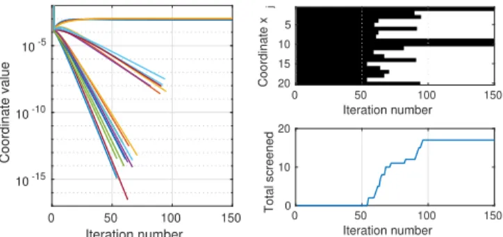
Accelerating the solution of the Lasso problem becomes crucial when scaling to very high dimensional data. In this paper, we pro- pose a way to combine two existing

Abstract – Various strategies to accelerate the Lasso optimization have been recently proposed. Among them, screening rules provide a way to safely eliminate inactive variables,

The present observational and retrospective study aimed at evaluating the screening rate of cervical cancer between 2006 and 2011 by age, place of location and for 3-years period

[r]

Fourth, it would be helpful, in particular for medical stu- dents and residents, if the authors could rank the relevance of the different topics within a chapter (e.g.,

and this during the dextral transpression in the simplon ductile shear zone (Fig. the folding of the schistosity, with the sW-directed stretching lineation, XII, can