A comprehensive numerical procedure for solving the Taylor-Melcher leaky dielectric model with charge evaporation

A comprehensive numerical procedure for solving

the Taylor-Melcher leaky dielectric model with

charge evaporation

by

Ximo Gallud Cidoncha

Submitted to the Department of Aeronautics and Astronautics

in partial fulfillment of the requirements for the degree of

Master of Science in Aeronautics and Astronautics

at the

MASSACHUSETTS INSTITUTE OF TECHNOLOGY

September 2019

@Massachusetts

Institute of Technology 2019. All rights reserved.

Signature redacted

A uthor .... . ... ...

Department of Aeronautics and Astronautics

September 2019

Signature redacted

C ertified by ...

Paulo C. Lozano

M. Alemain-Velasco Professor of Aeronautics and Astronautics

Thesis Supervisor

Signature redacted

A ccepted by ...

....

MASSACHUSEITSUINTTE

_{Sertac Karaman}

Associate Professor of Aeronautics and Astronautics

OCT

0 9

19

Chair, Graduate Program Committee

A comprehensive numerical procedure for solving the

Taylor-Melcher leaky dielectric model with charge

evaporation

by

Ximo Gallud Cidoncha

Submitted to the Department of Aeronautics and Astronautics on September 2019, in partial fulfillment of the

requirements for the degree of

Master of Science in Aeronautics and Astronautics

Abstract

Electrosprays in the pure-ion mode are of particular interest to space propulsion be-cause of its ability to produce high specific impulse and efficient electrical-to-kinetic energy transformation, together with its simplicity and compactness.

Unlike electrospray emitters operating in the droplet mode, pure-ion emission is known to be very dependent on the meniscus configuration, and consequently permis-sible under specific circumstances, mostly related to its stability. This has conferred pure-ion sources with an increased difficulty in controlling and predicting fundamental beam characteristics such as current emitted, while also making it hard to establish thec onditions that need to be met by the device structure to support adequate ion emission.

The use of Ionic Liquids has moderately alleviated some of these limitations, but still, the physics that lie behind electrosprays in the pure-ion regime remain consid-erably elusive.

This lack of fundamental knowledge has motivated past research on multiphysics simulation frameworks, mostly based on a modified version of the Taylor-Melcher leaky-dielectric model to account for the characteristics of charge evaporation in the pure-ion regime.

Findings in these frameworks have unveiled a family of stable solutions for the problem of a volumetrically-unconstrained emitting source. Stability is found under specific sets of circumstances involving structure of the feeding architecture that favours high hydraulic impedances, small meniscus characteristic lengths and limited range of op-erating voltages.

The lack of previous work has limited validation efforts in the literature to sim-plified physical models and a limited subset of physical input parameters. Besides, implementation limitations of commercial solvers (e.g, meshing resolution and no par-allelization), have hindered the exploration of menisci stability in important ranges of parameters such as high contact line radius or high values of the external electric field. In this thesis we provide a comprehensive numerical finite element framework to solve the Taylor-Melcher leaky dielectric model with charge evaporation to find static equilibrium shapes of pure-ion emitting meniscus, we validate the shapes obtained with the results in previous work and provide an updated stability map for steady evaporation.

Thesis Supervisor: Paulo C. Lozano

Acknowledgments

I dedicate this thesis to my parents, for their unquestionable love, support and strength during my whole life. I am feeling this powerfully, even with a 6000 km wide ocean separating us.

I would like to first thank Professor Paulo Lozano, my advisor, for his patience, invaluable insight and unbeatable encouraging skills. I would like to make special reference to his ability to motivate his students by constantly reminding us how our research work is contributing to enable the next generation of nanosatellites. I would also like to thank Professor Jaume Peraire for his advice in numerical modeling.

My life in Cambridge would not have been the same without my friends from

Spain, which have helped me to feel that little piece of home we often need to feel.

I would like to thank my Space Propulsion Lab friends to create such a great day

to day environment.

I would also like to thank Obra Social La Caixa, for funding my studies here at

the Space Propulsion Lab and believing in my dream of making the outer space a more democratic place for everyone.

Contents

1 Introduction

1.1 Context and electrospray basics: the Taylor cone . . . .

1.2 From pure droplet emitting cone-jets to pure ion emitting sources

1.3 Applications of the pure ion regime . . . .

1.3.1 Potential of Ionic Liquids for micropropulsion ion sources . 1.4 Research gap and brief literature review . . . .

1.5 Thesis objectives . . . .

2 Problem description

2.1 Problem overview . . . . 2.2 Domain definitions . . . .

2.3 Characteristic orders of magnitude of current evaporation . .

2.3.1 Critical field of emission (E*) . . . . 2.3.2 Characteristic evaporation region (r*) . . . .

2.3.3 Characteristic evaporated current and current density 2.4 Equations fulfilled in the bulk domain . . . .

2.4.1 Electric problem . . . .

2.4.2 Fluid problem . . . . 2.4.3 Energy problem . . . . 2.4.4 Summary of bulk physics . . . .

2.5 Equations fulfilled at the meniscus or liquid-vacuum interface ('M) 2.5.1 Summary of equations fulfilled at the meniscus interface (l7m)

2.5.2 Boundary conditions at the rest of the edges of the domain .

15 . 15 . 17 . 18 . 20 . 21 . 23 25 . . . . . 25 . . . . . 26 . . . . . 27 . . . . . 28 . . . . . 29 . . . . . 29 . . . . . 30 . . . . . 30 . . . . . 32 . . . . . 33 . . . . . 34 34 38 39

3 Numerical procedure

3.1 O verview . . . .

3.2 Variation of electrical conductivity and viscosity with temperature 3.3 Non-dimensionalization . . . . 3.4 Electric problem . . . .

3.4.1 Non dimensional equations solved . . . . 3.4.2 Non-dimensional numbers . . . . 3.4.3 Derivation of the strong form . . . . 3.4.4 Proposed solution method 1 . . . . 3.4.5 Other possible methodologies . . . .

3.5 Fluid problem . . . . 3.5.1 Non dimensional equations solved . . . .

3.5.2 Non-dimensional numbers . . . .

3.5.3 Strong form . . . . 3.5.4 Proposed solution method 1 . . . .

3.5.5 A note about the finite element discretization 3.5.6 Other possible methodologies . . . .

3.6 Energy transport problem . . . . 3.6.1 Non dimensional equations solved . . . .

3.6.2 Non-dimensional numbers . . . .

3.6.3 Strong form . . . . 3.6.4 Proposed solution method . . . .

3.7 Surface update . . . .

of 3.51

3.7.1 Stopping criteria for statically stable solutions found

3.7.2 Stopping criteria for no solutions found . . . .

3.7.3 Methodology 1 . . . . 3.7.4 Methodology 2 . . . . 3.8 Implementation details . . . . 3.8.1 Meshing . . . . 3.8.2 Parallelization . . . . 43 43 44 44 . . . . 46 . . . . 46 . . . . 47 . . . . 48 . . . . 50 . . . . 58 . . . . . 59 . . . . . 59 . . . . . 59 . . . . . 60 . . . . . 60 . . . . . 64 . . . . . 65 . . . . . 65 . . . . . 65 . . . . . 66 . . . . . 66 . . . . . 67 . . . . . 68 . . . . . 69 . . . . . 70 . . . . . 72 . . . . . 73 . . . . . 79 . . . . . 79 . . . . . 82

3.9 Sum m ary . . . .

4 Results 85

4.1 V alidation . . . . 85

4.1.1 Validation of electrical physical magnitudes . . . . 88

4.2 Velocity and temperature distributions along the meniscus . . . . 90

4.3 Shape dependence on o and B . . . . 91

4.4 Current dependence on

E

and B . . . . 93

4.5 Contact angle variation with

E

and B . . . . 96

4.5.1 Contact line singularity in in

El

and & . . . . 96

4.6 Lim its of Stability . . . . 99

4.6.1 Influence of the temperature dependence of k and y in the sta-bility boundaries . . . . 101

4.7 Numerical convergence analysis . . . . 102

4.8 Computational time reduction due to parallelization . . . . 103

5 Conclusions 107

List of Figures

1-1 Image of the cone-jet region of a Taylor cone, extracted from

[38]

16

1-2 Propulsive efficiency and total charge-to-mass fraction (qt/mt) for dif-ferent values of ion mass fraction. For E = 0.01. . . . . 19 1-3 Propulsive figures of merit as a function of current ion fraction. . . 20

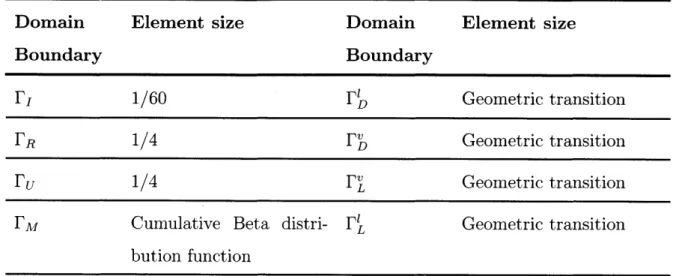
2-1 Computational domain diagram, boundary nomenclatures and carac-teristic dimensions of the problem. . . . . 26 3-1 The Cumulative Beta distribution for several values of p, q has allowed

us to build refined meshes along the meniscus ensuring a smooth tran-sition between nodes . . . . 81 3-2 Numerical procedure diagram for obtaining an equilibrium surface for

given

E

0, $, CR, B and an initial guess F' . . . . 84

4-1 Comparison between non dimensional equilibrium surface data for two different values of the operational space. The rest of the parameters

correspond to CR = 103 and Pr = 0 . . . . 86

4-1 Comparison between non dimensional equilibrium surface data for two different values of the operational space. The rest of the parameters correspond to CR = 103 and Pr = 0. . . . . 87

4-2 Comparison between non dimensional electric potential and surface . The rest of the parameters correspond to CR= 103 and §, = 0 _{. . . . 89} 4-3 Non dimensional temperature distribution along for different sample

4-4 Non dimensional velocity distributions in the normal and tangential

direction for different sample contact line radius. CR= 103 . . . . . . . ₉₁

4-5 General description of the equilibrium shapes in the emitting region for fixed external electric field and fixed contact line radius respectively. Plots corresponding to CR = 103 reference to the continuous lines whereas the dashed lines correspond to CR=. 104. . . . . . . . . . . . 92

4-6 I-Fo curves for different values of B and CR. Continuous lines

corre-spond to CR = 103. Dashed lines correspond to CR = 104 . . . . 94 4-7 Contact line angles as a function of E for different values of B and

CR. Continuous lines correspond to CR = 103, dashed lines correspond

to CR = 104. . . . .

97

4-8 Normal component of the electric field distribution (continuous) and

surface charge (dashed) along the meniscus for B = 0.0467, CR = 103, X, = 0 for different values of o . . . . 99

4-9 Limits of stability as a function of

Eo

and B for values of CR = 103

and CR = 10 . .... .---- -... .-.....----.. -. 100

4-10 Plot of expression 4.1 for different values of the non-dimensional electric conductivity sensitivity (dotted vs. continuous line

)

and different values of the temperature variation order of magnitude (blue vs. red). 102 4-11 Numerical convergence test as a function of relaxation parameter

#.

. 105

4-12 Computational time spent per iteration k as a function of the number ofCPUs.CR103

List of Tables

2.1 Nomenclature and symbols . . . . 27

2.2 Equations fulfilled at the bulk domains . . . . 34

2.3 Equations fulfilled at the interface . . . . 39 3.1 Non-dimensionalized equations enforced each iteration in the electric

solv er . . . . 4 7

3.2 Non-dimensionalized equations enforced each iteration in the fluid solver 59

3.3 Non-dimensionalized equations enforced each iteration in the energy transport solver . . . . 66

Chapter 1

Introduction

1.1

Context and electrospray basics: the Taylor

cone

This thesis is situated in the context of electrospray emission. An electrospray is a device that uses high electric fields to extract matter from conductive fluid surfaces. The most common form of an electrospray consists of an emitter (usually a long capillary tube or needle) at the end of which a liquid meniscus is formed. A high voltage difference is applied between the emitter and an extractor electrode situated at a certain distance from the emitter. When the external electric field in between the electrodes is sufficiently strong, the interface of the fluid and the external di-electric medium (often vacuum but sometimes air or even another liquid) chaotically transforms its geometry into a cone-like structure or Taylor cone [43]. The cone-like geometry is stable over a range of electric fields and guarantees the balance between the electric force traction and the pulling nature of the surface tension.

Geoffrey Taylor demonstrated in [43] that when both, differences in hydrostatic pressure between the liquid and the external dielectric medium and space charge also in the dielectric medium were neglected, the interface approached a perfect conical

geometry of semiangle6T= 49.29 in the ideal situation where the cone is static, thus

experi-mentally for many cases to a very good approximation, despite the aforementioned assumptions. The normal component of the electric field to the interface in the vac-uum side E is known to be:

E = ot0 T(1.1)

Where Eo is the vacuum dielectric perimittivity - is the surface tension coefficient of the liquid and r is the distance between the apex of the cone and any point along its generatrix.

The singular behaviour of the electric field created near the apex (E ~ causes the cone to break in a thin jet (see figure 1-1) that breaks into droplets down-stream as a result of capillary Rayleigh instability [36].

Figure 1-1: Image of the cone-jet region of a Taylor cone, extracted from [38]

Fernandez de la Mora et al. [12] derived a closed expression for the total current emitted I from the jet which is independent from the voltage applied, electrode ge-ometry and fluid viscosity. The expression is derived from equating the characteristic fluid passage time through the transition region of the cone-jet to the character-istic charge relaxation time and considering that surface charge distribution o is relaxed along the interface (o-= oE ). The droplet current emitted I has the following form:

I =f (Er) - Q(1.2)

Where r,, is the characteristic length scale of the jet, E, is the relative dielectric permittivity of the liquid,

f

(Er) is an empirical function.

Q

is the fluid flow rate and

Similarly, other expressions based on the characteristic length scale r,

Q

and equation 1.2 can be derived for magnitudes such as the jet width, emitted droplet size, and the droplet charge per unit charge [15].

1.2

From pure droplet emitting cone-jets to pure

ion emitting sources

The experimental validity of equation 1.2 holds when the non dimensional number is relatively high (I >> 1). When the flow rate becomes sufficiently small, namely T is reduced, the maximum electric field along the cone-jet surface

E' (e.g, the electric field near the transition region from cone to jet) starts to

increase (Ev oc 1 [13]). If En is sufficiently large and greater than a threshold electric field or critical field E* (on the order of 1 ~ 2-), a process known as

field evaporation [29] begins to compensate the loss of droplet current (I oc v/Q) by

releasing low-solvation ions from this transition region. In summary, the material ejected from the electrospray in these conditions is a mixed beam of droplets and ions that is characterized by two different ranges of specific charges.

If the parameter T is further reduced, the jet dimension decreases sufficiently so

that the proportion of current emitted through droplets starts to be comparable to that of the ions evaporated. Under certain conditions, if the flow is further reduced to levels where T < 0.5, the jet becomes unstable until the point where droplet emission

is no longer sustained. On the other hand, ion emission will continue increasing until the extent to which only ions are emitted from a stressed, closed-surface of the liquid. This electrospray mode is known as the Pure Ion Regime (PIR). In fact, the total PIR current will also increase because ions can transport charge much more effectively than droplets for a given mass flow (greater -). The PIR mode is known to exist only for limited types of fluids such as liquid metals [41] and ionic liquids [30].

1.3

Applications of the pure ion regime

The main motivation of this thesis is the application of the PIR to electric micro-propulsion. Pure ion sources can be very interesting because of its ability to access to high specific impulse propulsion regimes at maximum attainable efficiency. Assume an electrospray propulsion system working with a monodisperse mixture of droplets

(d) and ions (i). The propulsive efficiency (ratio between propulsive power and input

power) is assumed to be the main source of losses. It yields:

F2

r/, = (1.3)

Where F is the total thrust, rh is the total mass flow rate ejected from the thruster, I is the total power and V the nominal accelerating voltage. If

N

is the total number of particles of type

j

ejected per second (j = {i, d}) then:

F= Ncimi + Nacdmd (1.4)

rm= Nimi +

Ndmd

(1.5)

I = iq_i + Ndqd (1.6)

Where c 3- 3v is the maximum velocity reached starting from a particle

jof

charge qj and mass mj at rest, and assuming a free fall acceleration through the nominal potential difference V. Substituting the previous expressions in equation 1.3 yields:

rIP - imJ + Ivdyqdmd} 2 (1.7)

(Aiqi +N2dqd) (k i+N dmd) 1-(1 )ii

Where 3i = 'f = _I - , - is the fraction of ion current to total

Ii+Id Ii+Id Niqi+Ndqd

current emitted, ande= "qdd is the ratio between droplet and ion charge to mass ratios.

We also can obtain an expression for the specific impulse

(Ip)

of a monodisperse propellant mixture of ions and droplets as a function of the current fraction of ions

1 0.8 7 0.8 qt/mtat /mi 0.6 0.4 0.2 0 0 0.2 0.4 0.6 0.8 1

Figure 1-2: Propulsive efficiency and total charge-to-mass fraction (qt/mt) for different values of ion mass fraction. For e = 0.01.

3, if we substitute the parameters in equations 1.4, 1.5 and 1.6:

F q 1-(1-V7)#i

gISP =- 2V-- (1.8)

m md -1 e#

Where g is the gravitational acceleration at the Earth's surface. The figure 1-2 illus-trates the two efficient regimes at none and pure ion fraction, with poor performance in between. The reader can observe also that the maximum specific impulses in figure 1-3a are obtained for a pure ion regime, as suggested because its maximum charge to mass ratio (see figure 1-2). Operating at high specific impulses is very useful for high

AV budget missions, as the propellant mass to attain the AV budget is decreased:

mpoeun= 1 -e9S (1.9)

mtotal

Figure 1-3b shows different propellant mass fractions as a function of the specific impulses for a given AV.

Other applications of the pure ion regime include focused ion beams (FIB) for etching and deposition [34] or ion microscopy [27].

Specific impulse for various values of accelerating potential -V = 1000 Volts - V = 5000 Volts !- V = 10000 Volts 1 0.8 0.6 0.4 0.2 nI 0 0.2 0.4 0.6 0.8

Propellant mass fraction for various values of mission Av budget

- V = 100 m/s -- AV = 1000 m/s --AV = 10000 m/s

1 0 0.2 0.4 0.6 0.8 1

(a) Specific impulse as a function of current (b) Propellant mass fraction for different val-fraction of ions 3 for different values of accel- ues of Av. For e = 0.01 and - - 106. erating potential. For c = 0.01 and-1- - 106.

Figure 1-3: Propulsive figures of merit as a function of current ion fraction.

The use of liquid metal ion sources (LMIS) as a propellant for pure ion

micro-propulsion (Field Emission Electric Propulsion, FEEP [3]) has been in the focus of research in the past decades due to its benefits of combining very low thrust and

very high specific impulses. Electrospray propulsion based on FEEP systems often

represent the most viable option for drag-free satellite applications in missions such

as LISA Pathfinder [42] and Microscope [31], where an accuracy in thrust about

(0.1 pN) over a relatively wide thrust range (0.1 - 150 pN) is required. The use of

LMIS is particularly suited for these missions, they are characterized by a relatively

high current requirement (on the order of > 1 mA).

1.3.1

Potential of Ionic Liquids for micropropulsion ion sources

Ionic liquids (ILs) are a type of molten salts that remain liquid at room temperature because of the strong coulombic interactions among their molecules. Despite having smaller conductivities than LMIS, PIR modes are relatively straightforward to obtain

[18, 29]. ILs' range of current throughput resides between 100 nA to 1000 nA, approximately 2 orders of magnitude less than the output of common LMIS. This limitation can be mitigated by the use of arrays.

15000

-

10000-5000

ILs are of particular interest also because of its versatility. Up to 108 combina-tions of anions/cacombina-tions are reported to be possible at least for industrial applicacombina-tions

[35].

This versatility gives access to a wide range of cation and anion pairs to tune both physical properties and specific molecular chemistries useful for propulsion. For instance, generation of heavy mass ions is desired to maximize the thrust-to-power ratio (Lc 77). Furthermore, IL-based propulsion systems have the potential for high-efficiency propulsion, as no energy has to be spent on propellant liquefaction neither on propellant ionization, since molecular ions are readily extracted from the propellant bulk. Microthrusters based on ionic liquids can also produce both posi-tive and negaposi-tive ions. This is beneficial for spacecraft charging issues, as average neutralization can happen simply by operating the thrusters in alternate polarities

[33].

1.4

Research gap and brief literature review

Unlike LMIS, where space charge apparently enhances the stability of the meniscus

by shielding the effects of external electric perturbations, ILs space charge effects

are negligible, which makes the quality of the source more susceptible to the specific properties of the working ionic liquid and emitter geometry [6].

The experimental difficulties of resolving properties like the meniscus interface profile, fluid interaction with the tip and characteristics of internal creeping flow have hindered a clear understanding of ILIS, specially the role of key operating parameters such as the external electric field, size of tip inlet pores or hydraulic impedance of the feeding material in the total current emitted or meniscus stability.

On the computational side, there are two major attempts in the literature to ap-proach this problem. Higuera [19] modeled a very small ionic liquid drop under steady charge evaporation attached to a flat conducting plate. The equations were adapted from the Taylor-Melcher leaky dielectric model [40] including charge evaporation. No initial equilibrium shape was assumed. First of all, a Laplacian field equation was solved in both, the region outside the attached droplet and the droplet itself together

with a free surface charge conservation equation at the interface. No space charge was considered. Electrical Maxwell stresses from the Laplace fields and surface tension were stated as boundary conditions for a Stokes flow solver. By using the interfa-cial velocity distributions coming from Stokes flow and a second order Runge-Kutta temporal discretization, Higuera propagated the interface along time-steps.

Higuera considered two meniscus cases. In the first case, the volume was constant. Higuera shows stationary solutions of steady evaporating menisci, surface charge and electric field as a function of a dimensionless volume parameter. A sketch of the starting voltage concept is seen in the I-V traces, which is experimentally consistent. The current increase with the electric field yields a linear behaviour before it gets unstable for a particular electric field. The same scaling relationship is reported by a large number of empirical studies and it is believed to be due to the limits in conductive charge transport within ionic liquids [26, 30, 9].

In the second case, Higuera considered an external reservoir capable of pumping fluid with pressure po towards the meniscus, and the pressure drop that occurs because of friction of the fluid with the channel walls that connect the reservoir to the external electrodes (hydraulic impedance coefficient a). The non-dimensional total current emitted versus non-dimensional field was shown to be very dependent on po and a, yielding currents with very dissimilar behaviour (up to 3 orders of magnitude difference for apparently close values of po and a). Regardless of the limitations of Higuera's model, the author was able to depict the notion of a maximum external field, which suggests that purely ionic emission might only be permissible within a narrow band of stability. The numerical variability for the current in the second case as a function of po and a points out the importance of upstream conditions in determining emission behavior, which is in agreement with experimental work.

Coffman

[7]

updated Higuera's model by removing any volumetric constraint. The author also considers a substantial fraction of the liquid feeding system in the computational domain, which is a more realistic description of an actual ILIS than a droplet attached to a flat plate. Coffman considers also Ohmic heating effects, which were disregarded by Higuera.

Coffman was able to reproduce the solutions of Higuera by reduction of the free-volume model to a constrained free-volume and translating the non-dimensional param-eters to the author's framework. Coffman was able to show that Higuera's menisci were practically hydrostatic and the surface charge distribution was practically re-laxed due to the facts that they were particularly small (the characteristic size of the emission region is only a moderate fraction smaller than the contact line), the capillary number was low and the dielectric constant was particularly high (on the order of er = 50). For this reason, the hydraulic stress tensor was found not to play

any substantial role in the interface shapes or emission strengths. It was shown to be even decoupled from the iteration process.

Coffman described the static equilibrium shapes and associated physical magni-tude distributions (surface charge, current density, electric fields ... ) as a function of a set of operational space parameters, namely the electric field downstream, contact line radius and a hydraulic impedance coefficient. These operational space descriptions

went in substantially more detail than Higuera (specifically concerning the contact line radius parameter). The author was able to describe qualitative trends also seen in experimental work. For instance, the existence of a low electric field non-evaporative lower branch of solutions with a turning point at certain value of the electric field where the meniscus starts emitting [22]; stable solutions for relatively large values of the contact radius [6, 37] and inverse proportionality between hydraulic impedance

and total emitted current [30].

Owing to the lack of computational power and the constraints imposed by com-mercial solvers (mesh resolution limitations, no parallelization), Coffman was only able to modestly populate the stability diagram up to a few values of contact line radius (1, 2.5, 4, 4.5 and 5 pm) for two different hydraulic impedances.

1.5

Thesis objectives

In this thesis, we have built our implementation of Coffman's model without any of the aforementioned limitations. That is, we integrate Gmsh

[16],

an open-source

meshing software, and FEniCS [1], a finite element method library that contains mesh partition algorithms to parallelize the solving mechanism and substantially accelerate the computational work.

The main contributions of this thesis are the following:

1. We propose and solve a finite element framework for all the different physics

involved in [7], including a new surface update process based on the least-squares minimization method.

2. We provide an updated version of the stability diagram in [7] for 4 different values of the hydraulic impedance and 16 different values of contact line radius.

3. Identifying the roadmap for future developments in the numerical simulation of

Chapter 2

Problem description

In this chapter we describe the computational domain in detail, we introduce the equations that will be solved and introduce the fundamental orders of magnitude of pure ion emission in ionic liquids.

2.1

Problem overview

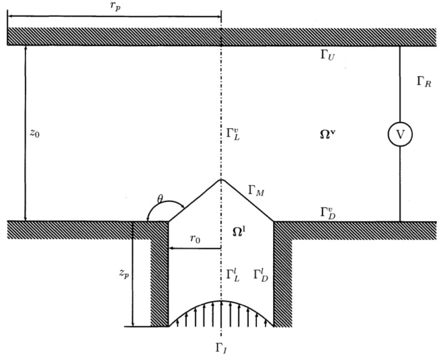
The reader can see a diagram of the problem domain in figure 2-1. In this problem we consider a column of fluid of radius ro that is attached to a downside electrode with the shape of a flat plate of dimensions rp. In this thesis, the plate considered is a conductor, but without of generality, this plate can be a dielectric of relative electrical permittivity Er. The downside electrode is biased with a potential difference AV with respect to a flat upside electrode at a distance zO, so that an electric field exists in the region in-between. The fluid column can be understood as a tube connecting the open space between the two electrodes with a fluid reservoir at pressure pr. This reservoir is not treated computationally. The fluid enters the computational domain as if it were the outlet of a fully developed pipe flow (Hagen-Poiseuille paraboloidal flow). It is accelerated through the vicinities of the emission region close to the tip and released to the external vacuum region in form of evaporated ions.

We consider the same situation as

[7],

where the the liquid column contact line with the downside plate is fixed (pinned), while the contact angle is free to adopt any

value. The objective of this problem is to find what is the axisymmetric meniscus shape Fm of contact line radius ro that is in static equilibrium supporting steady evaporation of ions. In other words, which is the shape whose associated surface energy or surface tension balances the electric pushing stress and the hydrodynamic fluid stresses for a situation of steady evaporation.

PU zo I L FR

0

zp rv

bD

rM L D

Figure 2-1: Computational domain diagram, boundary nomenclatures and caracter-istic dimensions of the problem.

2.2

Domain definitions

In this section we provide the proper nomenclature and definitions we are going to use along the following parts of this thesis. The reader can see the diagram in figure 2-1 to identify the location of the different regions.

rp

Table 2.1: Nomenclature and symbols

Symbol Description Symbol Description

QV Bulk open vacuum domain Q1 Bulk open liquid domain

(Qv c R2₎

(Qj c R2)

J'v Axis of symmetry in the vacuum I" Axis of symmetry in the liquid side (Left side of the axisymmetric side

computational domain in figure

2-1)

IF Inlet of the fluid column 179 Downside electrode (non-wetted, in the vacuum side)

F.A Liquid-Vacuum interface (Menis- FR Right side of the domain (far from

cus) the meniscus)

Fl Downside electrode (wetted, in FU Upside electrode the liquid side)

(9Q" Boundaries of the open vacuum 8Q, Boundaries of the open liquid do-domain (&O, := F1 U F7 U FD U main (O, FDUFU UF)

FR U rU)

2.3

Characteristic orders of magnitude of current

evaporation

Before seeing all the equations that play a role in the steady evaporation of charge

from a closed meniscus, we can define some representative orders that will allow us

2.3.1

Critical field of emission

(E*)

Iribarne and Thomson [20] suggested that charge emission in high conductivity fluids like liquid metals and certain ionic liquids (under special circumstances) obeys a phenomenological Arrhenius rate equation of the following shape:

e kBT (Ea (2.1)

n h _kBT)

Where

j=

ji

is the local current density emitted at the surface of the meniscus,

kBis Boltzmann constant and Ea is an activation energy, T is the liquid temperature, h is Planck's constant, and Ea is the characteristic activation energy. The activation

energy (referred also as AG solvation energy, see [18]) for most of the ionic liquids is very high (1 - 2 eV). For this reason, most of them do not experience significant

thermal evaporation at room temperature and remain liquid. The presence of strong electric fields near the tip of the meniscus is known to lower this activation energy barrier:

Ea = AG - G(E") (2.2)

Where En is the external local electric field perpendicular to the meniscus surface. An image charge argument can be brought into consideration when analyzing the dependence of G(Ev) with respect to the external electric field E". In the limit of planar geometry this function's scaling can be approximated to:

esEn

GE(E) = e (2.3)

F47rEo0

When G(En) ~ AG, the evaporation kinetic process (equation 2.1) is activated and the meniscus tip region starts emitting charge. We can give an estimation of the value of this critical electric field from which the closed meniscus will start emitting

charge:

E 47rEo (AG)2 (2.4)

2.3.2

Characteristic evaporation region (r*)

If we model the emission region of the meniscus as a spherical cap and neglect any

hydrodynamic pressure, the balance of stresses in the normal direction should be:

1 O " _ o 1 2 2 27

1EE n oer = -*

2 2r (2.5)

Where r* is the radius of this spherical cap, and E, is the internal local electric field perpendicular to the meniscus surface. It can be shown ([7]) that in this region, the ionic liquid meniscus behaviour approaches that of a perfect dielectric fluid where

E', ~ . If the meniscus is emitting, it will adapt its surface shape so that En E*.

Esr

Using these two assumptions, the balance of stresses in equation 2.5 yields:

SeoE*2Er - 1

2-2 Er

r*

(2.6)

For typical ionic liquids where E >> 1, the characteristic emission radius yields: 4_7y

r* =

4-T' E0E*2 (2.7)

Where r* is on the order of 10- - 10-'0 m.

2.3.3

Characteristic evaporated current and current density

If we consider the region of evaporation as a spherical cap then the total current

emitted can be stated as:

1 kE* )2 327rk y 2

I* j*A = kE -=- _27r (r*)2 2 2

Er EOEE (2.8)

where

j*

~ kE ~ is the characteristic current density in the emission region. k is the electrical conductivity and A = 27r (r*)2 is the area of the spherical cap. For typical ionic liquids * is on the order of 50 to 500 nA.

2.4

Equations fulfilled in the bulk domain

In this subsection, we will describe the set of physical equations that govern the physics in the bulk vacuum (d) and liquid (Q1 ).

2.4.1

Electric problem

Maxwell-Faraday steady state equation

In electrostatics, this equation takes the well-known following form [17]:

V x E = 0 (2.9)

Which implies that the electric field can be expressed as the gradient of a potential function

#:

V x = 0 -

E=-V

(2.10)

Maxwell-Poisson constitutive equation

The constitutive equation for electrostatics is the equation of Maxwell-Poisson equa-tion for linearly polarized media [17]:

V - (EOsEr) = pch (2.11) Where Eo is the vacuum electric permittivity, Er is the relative electric permittivity of the material with respect to vacuum, and Pch is the space free volumetric charge. In this thesis, we consider the simplifications made by [7] with respect to the space charge (Pch) in both the liquid (Qj) and vacuum domain

(Q,)

(see next section).

Space charge considerations (Pc) in the liquid domain (Qj)

Ionic liquids can be considered to be quasi-neutral in the bulk for an emitting situation (all the net free charge has migrated to the surface). As in [7], we can give an

estimation to the transition layer in the bulk below:

V.oE ~cor-- (n+ -_) (2.12)

Typical values for ion emission for the electric field (IAE I 109 ) and ion concen-tration

(n

n-n ~ 1028 ) yield an order of magnitude for the near-surface charge

layer of 6 ~ 10-- 1< 0-7, which is the typical lower bound of the meniscus sizes considered in [7, 19]. For this reason, we consider an quasi-neutral space charge

envi-ronment in the whole bulk liquid domain, except a surface charge distribution along 1 , o, which we will describe later on. Given this consideration the source of space

charge Pe in the liquid will be purely given by the differences in mobility due to temperature effects.

Space charge considerations (ch) in the vacuum domain (Q)

As suggested in [7], we can neglect the effects of space charge of ions being evapo-rated at the vicinity of the meniscus tip. Coffman et al. [8] give an order-of-magnitude argument based on characteristic current, electric fields and length scales of evapo-ration to estimate the effects of space charge. In particular, the electric field near the emitting tip ( ti), which is on the order of the critical field (Etip, E* can be approximated to the sum of a homogeneous Laplacian field (Eh) and a pertur-bation field caused by the space charge (Ec). That is, |Etjp| ~

IEh

+Escl ~ E* The ratio between the space charge induced field and the critical field can be shown to be approximately the ratio of the characteristic residence time for a particle in electrostatic free-fall around the tip( ~ E*r* to the charge relaxation

time(y). ~~ ~ 8ryo, [7]. If we substitute the physical

parameters with the ones particular to ionic liquid emitters (I 10-8 ~ 10-9

k = 1 , -y = 0.05 N - m, - = 106 , E, = 10) we get an interval of variation for

F, ~ 10-2 10-1. _{We can consider space charge effects negligible in this situation.,}

the liquid domain argument, we can simplify equation 2.11 to Laplace equation:

V2_{# = 0 (2.13)}

Charge Conservation

The charge conservation equation in steady state is shown below:

V

j=

0 (2.14)

Where

j

is the current density vector. Equation 2.14 should be fulfilled in the liquid domain (Q). We can use Ohm's law [17] to complete equation 2.14:

V - (k) - 0 (2.15)

The fact that the electrical conductivity k is a strong function of temperature, k=

k(T), prevents equation 2.15 to be reduced to equation 2.13.

2.4.2

Fluid problem

Incompressible steady state Navier-Stokes equations

The Navier-Stokes equations for incompressible (p -± po) steady state fluids are the mass conservation equation:

V • = 0 (2.16)

And the momentum conservation equation:

p(' -V) = V -m (2.17)

Where p is fluid density, i the fluid velocity, m = _{-p+y(Vi+V) is the fluid}

stress tensor for a Newtonian fluid, p is the fluid pressure, I is the identity isotropic tensor, and p is the viscosity coefficient of the fluid.

2.4.3

Energy problem

Energy conservation equation

The conservation of enthalpy principle for fluid-state materials can be regarded as a convection-conduction transport equation and it is generally written as follows:

ii. Vh = -V 4 + (2.18)

Where h is the enthalpy per unit volume,

4

is the conduction heat flux and

e

is a heat source per unit volume.

Enthalpy per unit volume (h)

Due to the high density of fluids. the enthalpy per unit volume can be related to the temperature using a linear law of the following form h = pcpT. Where c, is the

specific heat at constant pressure and T is the temperature of the fluid.

Heat flux (4)

We consider Fourier's law in this thesis for heat conduction which has the follwing form:

4

= -kTVT (2.19)

Where kT is the thermal conductivity.

Heat source (e)

There are two potential sources of heat generation: viscous and Ohmic heat genera-tion. In this thesis we ignore viscous generation, which should be weak as a result of the tenuous flow. Thus:

S= (2.20)

The energy equation considered in steady state and with constant electric conductivity will be:

(2.21)

pci - VT = kTV 2_{T +L}

k

2.4.4

Summary of bulk physics

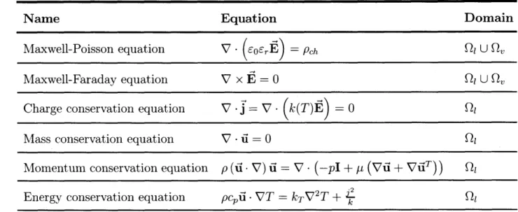
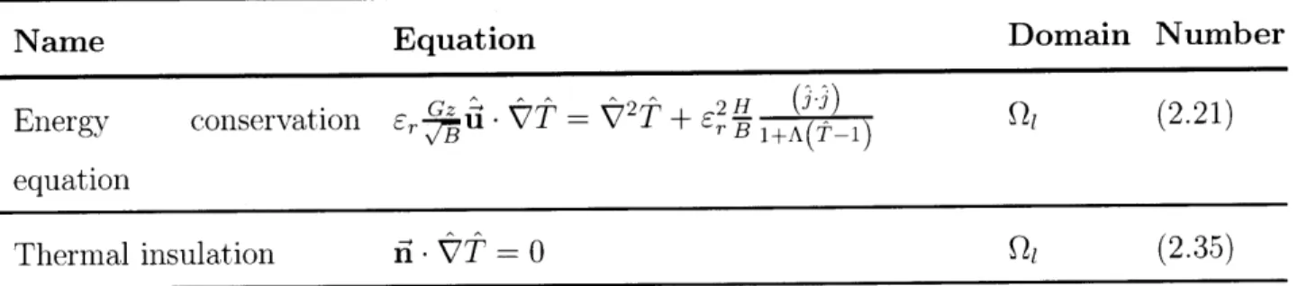
We provide a summary table for all the equations fulfilled in the bulk domain. Table 2.2: Equations fulfilled at the bulk domains

Name Equation Domain

Maxwell-Poisson equation V -(oEr) = Pch U Q,

Maxwell-Faraday equation V x E= 0 Q, U Q

Charge conservation equation V-

j

= V - (k(T)Z)= 0

Mass conservation equation V - U=0 QL

Momentum conservation equation p (' - V) u = V - (-pI + p (Vu + ViT Q1

Energy conservation equation PCp - VT = kV2T + _k

Qi-2.5

Equations fulfilled at the meniscus or

liquid-vacuum interface

(Fm)

In this subsection we describe the sets of equations fulfilled at the meniscus surface in equilibrium. These equations are additional to the ones stated in the previous subsection 2.4 and in table 2.2, which are also fulfilled in FM.

Equilibrium of physical stresses in the normal and tangential direction

The normal and tangential components of the stress acting on the fluid interface are, respectively:

(2.22) n - (e -rm) - V -n

(,e -m) (2.23)

Where n and t are the outward (pointing from Q1 to Q,) normal and tangential vector

to the surface, respectively; e and m are the electric and fluid viscous stress tensors,

respectively; -yV - describes the surface tension stress with linear coefficient -.

Electrical stress tensor and its expansion in cylindrical axisymmetric co-ordinates

The bulk electrical stress tensor for linearly polarized media (see for instance Melcher

[32] or Landau [24]) can be written as:

e = E0Er EiEj -- E (2.24)

Where Ej is the th cartesian component of the electric field, and 6

oj

is the Kronecker

delta function (6oj= 1 ifi =

j,

= 0 if i

j).

When the stress tensor is evaluated at an interface between two linearly polarized material (namely vacuum, 7e, and liquid, 7.), the electric stress tensor takes the following form:

e = e' - e = E - E -- Eos

(EE

- E (2.25)

Where E : Q1, E : Ov are the cartesian Ith components of the electric field in the liquid and vacuum respectively.

If we expand this tensor in an axisymmetric domain (r, z), it takes the following form:

T(E 2 -Ev2) - E 2 - 2E E7E - erEE'

=EE - r E E j(E)2- E2))- 2 E12 - E 1)

(2.26)

It can be demonstrated by simple algebra that the normal and tangential components of the electrical stress at the interface, that is, the products n -F. -n and . i-=e-n

respectively can be written as:

n Te- = o(EX2 - ErEi+7) o (,- 1)E 2 _(2.27)

t -r - EE - osEo Et = c-Et (2.28)

Where n = (n,nzt), t= (trtz) (n, -nr) are the normal and tangential vectors to

the interface (particularized for cylindrical coordinates). For the sake of clarity we define the normal component of the electric field in the vacuum side: En = Ei - n, where

{E,

E}: Qv. Analogously, we define the electric field in the liquid side

El = El - -, where {En, El} :O; and the tangential vector Et EvE = -.

Surface Charge jump condition at the interface

We can derive the following condition for the surface charge at the interface from

expanding Maxwell-Poisson equation locally around an infinitesimal control volume

enclosing a differential of the interface (see [24]). This condition yields:

n = E"- EosE,1 (2.29)

Where - is the surface charge distribution along the meniscus interface (o : FM).

Equality of tangential electric fields along the surface

The previous steady state Maxwell-Faraday equation expansion around an

infinitesi-mal control volume also yields the following condition for the tangential electric fields

at the interface:

Kinetic law for charge evaporation

We will consider the same Arrhenius-like expression explained in the previous chapter in this problem. See [20] That is:

cakB AG - q

jn=

-q(2.31)Gexp

h kBT

Charge conservation equation

If there is no accumulation of charge over time (e.g, steady state,

),

the charge that evaporates at the surface of the meniscus must be transported by conduction (form the bulk of the domain) and convected from the vicinities of the surface, where an existing non-zero surface charge a exits. Notice that convection cannot come from the bulk domain, as we are considering quasi-neutrality of the ionic liquid.

Thus, the local current balance emitted at each point of the meniscus FM can be stated as follows:

jn = jconduction + jconvection (2.32)

Where 2.32 can be expanded in the following form (see Saville [40]):

jconduction =kE' (2.33)

iconvection n -V - - - VsU (2.34)

The convective charge transport (jconvection) contains two terms, the first one in which can be related to the rate of deformation of the surface shape (notice the presence of the Vi factor). The second term reminds us of the familiar convective part from the well-known total derivative of a variable in an eulerian frame of reference

(L).

In

this case, the curved domain where this equation is defined for, Fm, needs a special operator VS (I -- n x n) V acting on o. This operator acting on o, Vs, can be interpreted as the orthonormal projection of the gradient of & onto this same surface, in this case, FM. The variable 3 is a smooth extension of a in a neighborhood of the

surface (manifold FM). It can be demonstrated that if o (f) : Fm -+ R is a sufficiently

smooth function, then Vso- = t`. In other words, the derivative of - along the arc-length coordinate of the meniscus contour (s), multiplied by the tangential vector to the contour.

Thermal insulation equation

In this thesis we are considering the case where the meniscus surface acts as a thermal insulator, that is:

n • VT = 0 (2.35)

Equivalence between fluid velocity and current evaporated

The current evaporated

j',

which is normal to the surface of the meniscus, relates to the distribution of matter exiting the meniscus, and therefore, to the distribution of normal velocities at the surface. This equivalence between the charge evaporated and the mass leaving through the meniscus surface can be expressed mathematically as follows:

in

u - : q:= (2.36)

Where - is the ratio of charge over mass per ion evaporated.

2.5.1

Summary of equations fulfilled at the meniscus

inter-face (I'A)

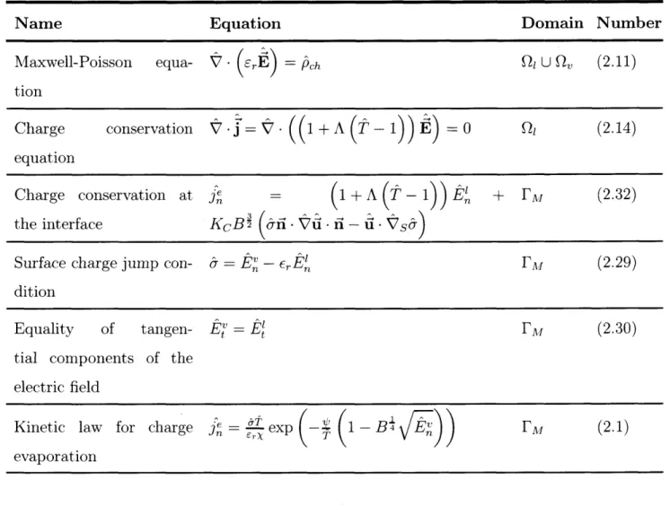
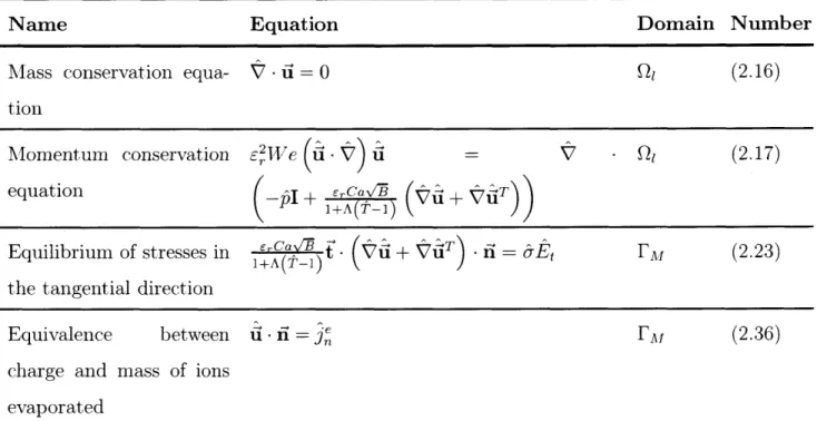
Table 2.3 shows the summary list of equations fulfilled at the interface.

Table 2.3: Equations fulfilled at the interface

Name Equation

Equilibrium of stresses in the normal di-

}o

(E,2 - eE4) + 1o(E - 1) E -2

rection (-p±+ ii (V+P + V -T) -) =-yV

Equilibrium of stresses in the tangential di- soEvEt - orEiEt

-rection (p -

(V

+ nG) = 0

Surface charge jump condition o =oE - EoErEi

Kinetic law for charge evaporation j exp

-Charge conservation = kE

+

o-ri V -* - i

Vso-Thermal insulation n' VT Equivalence between fluid velocity and u - = -2

current evaporated

2.5.2

Boundary conditions at the rest of the edges of the

domain

Electric problem

e Downstream electrode and inner fluid

(F,

I and F ): We consider the elec-trode as a conductor. The majority of the region of the liquid that does not emit can be considered to be at the same potential as the electrodes. In this case, we consider that the scale of the emission region (r*) is much smaller than the characteristic length of the inlet channel ro. For this reason, the region at the inlet also has this potential.

#=o

in F U IF U FV (2.37)

I I E

*Axis of symmetry (IF and It): Because the domain we are solving for is ax-isymmetric, a boundary condition for the potential field which is consistent

(symmetric with respect to the axis) is:

V# -fi = 0 in r1 U I

Justification of this boundary condition can be found at [4]. * Upstream electrode (Fu):

# = #0 + AV in Pu (2.39)

* Right hand side of the domain FR: We consider this region to be far away, thus unperturbed by the presence of the fluid column. Due to the planar electrode geometry the boundary condition is:

V0 - fi =- 0 in FR (2.40)

Fluid Problem

*Downside electrode (walls, IF): In this region in contact with the walls we have a no-slip condition:

u

= 0

_(2.41)

*Fluid inlet (F1 ): We consider fully developed pipe flow at the inlet, as the tube connecting the reservoir to the electrode region can be considered long enough (Ltbeb >> ro). For this reason, the boundary condition can be either one of the following.

- Neumann boundary condition for the fluid stress:

=1 In= Po4- Rh

Pm in F,

(2.38)

- Dirichlet boundary condition for the fluid velocity distribution and pressure reference: U, 0 in F1 S= -(b-- r2

₎

_in Fi (2.43) 4 0 P = Pr - IRh QRh in { (Xr,X,2) C FI

Where ur,u2 are the r and z components of the axisymmetric velocity vector

U, p, is the pressure at the reservoir, I

fj,

dS, is the total current that

the ion source emits (integral of the current density along the surface of the meniscus), Rh is the channel hydraulic impedance and

Q

is the total fluid flow rate (in ). Because the pressure is undetermined up to a constant, we need to specify a calibrating pressure at a point lying of the input boundary x

C

F,.

The pressure at the inlet is considered to be uniform along the channel (pipe flow), and equal to the pressure in the reservoir minus the uniform pressure drop originated by the friction of the flow with the walls.

•Axis

of symmetry (F1): For regularity of the solutions in an axisymmetric domain, we need the velocity field to be symmetric with respect to F . Following the structure of the electric problem, we provide a boundary condition for the fluid flow field which is consistent. Foundations and further discussion of this boundary condition can be found at

[25).

ur = 0 in F11

(2.44)

2 0 in _1L

Energy Transport Problem

*Downside electrode and fluid inlet (walls or F1, F): We consider the electrodes to be good heat sinks. For this reason, we can adopt a uniform reference tem-perature along the wall. We also consider the temtem-perature of the flow at the

regions far away from the emitting region to be equal to the wall temperature as well:

T = _TO (2.45)

The latter boundary condition for the inlet (F,) may be revised when exploring the regions of the operational space where the emitting region is comparable to the size of the inlet channel or computational domain.

* Axis of symmetry (IF'): We recall the arguments presented in the previous fluid and electric problems to justify the boundary condition at the axis of symmetry:

aT

VT -fi 0 (2.46)

Chapter 3

Numerical procedure

In this chapter, we provide a finite element framework to solve the set of equations described in the previous chapter.

3.1

Overview

The objective of the solver is to calculate which is the contour (FM) that is in static equilibrium or in other words, fulfills the equations described in the previous chap-ter for a given set of exchap-ternal conditions, namely the pressure at the reservoir (p,), external applied electric field (E), the radius of the channel (ro), and an hydraulic

impedance factor (Rh).

The solver is initiated with an initial guess of the axisymmetric contour (F), which is generally not in equilibrium. The initial guess is perturbed across several iterations (k) by using numerical minimization techniques. These perturbations will approach this Fk towards its equilibrium position.

We have divided the solver in four parts, the first three parts enforce equations be-longing to a particular physics, that is: electric, fluid and energy transport problems. The electric solver yields the distribution of electric fields along the meniscus (E, Fl and the surface charge (a). From there, we can calculate the electric stress tensor

(re),the distribution of current density that is being evaporated at the surface

j',

and

field (ii) and pressure distribution (p) along the surface of the meniscus. From there, we can calculate the viscous stress tensor(m). The energy transport solver yields the temperature distribution along the computational domain (T). The temperature plays a substantial role in both the fluid and electric problems, as the electrical

con-ductivity (k) and fluid viscosity (p) are strong functions of the temperature. The last

part of the solver uses the previously calculated tensor distributions and current to guess another IF that is closer to the equilibrium condition. This procedure will be explained in detail in the following sections.

3.2

Variation of electrical conductivity and

viscos-ity with temperature

For the purpose of this thesis, where we expect temperature magnitudes around the

room temperature (- 300 K), it is considered sufficient to model the dependence of the

variation of the electric conductivity with temperature using a linear approximation:

k(T) = ko + k'(T - T0) (3.1)

Where ko

()is

the electrical conductivity at the reference temperature (To) and

k' is a linear sensitivity coefficient

(i).

Since viscosity is inversely proportional to temperature (p(T) - T-1), we follow the same approach as Coffman

([7])

and take

p(T)k(T) = poko ~ as constant to capture this inverse proportionality behaviour, where yo is also a reference viscosity at room temperature.

We can then consider:

(T) = poko (3.2)

ko + k'(T - T)

3.3

Non-dimensionalization

In this subsection we will provide basic order-of-magnitude arguments to non-dimensionalize the equations described in the previous chapter.

* Length (r, z): We consider the radius of the channel ro as a characteristic length scale, thus the non-dimensional axisymmetric coordinates:

(r, ) = , -(3.3)

ro ro

* Pressure (p): We take as a reference pressure an estimation of the order of magnitude of the surface tension stress. As we have seen previously, the surface tension stress can be expressed as p, = yV -n. We can write this expression as

the sum of two terms involving the principal radius of curvature (i, K2) using

Meunsier theorem

[44],

that is:

P

p=-

, p =7V-= -n+ - (3.4)

p, i K2

The reference length for our problem is the channel radius ro. We then take the following reference pressure pc, as if the meniscus approached a perfect sphere of radius ro:

27y

Pc = - (3.5)

ro

" Electric field (E): In the limit of no evaporation and neglecting the pressure

drop along the channel, we have that:

1

EoE ~YV - n (3.6)

2

The order of magnitude for the surface tension should not be far away from the order of magnitude of the electric pressure. For this reason, we take the reference electric field Ec as:

^

E

'FT47

E - Ec - - (3.7)

Ec' so E roso

Once the scale of the electric field is set, other directly-related physical magni-tudes to

E

can be obtained: