Complex materials handling and assembly systems.

November 1, 1978 ESL-FR-834-7

COMPLEX MATERIALS HANDLING AND ASSEMBLY SYSTEMS Final Report

June 1, 1976 to July 31, 1978

Volume VII

ANALYSIS OF TRANSFER LINES CONSISTING OF TWO UNRELIABLE MACHINES WITH RANDOM PRO-CESSING TIMES AND FINITE STORAGE BUFFERS

by

Stanley B. Gershwin Oded Berman

This research was carried out in the M.I.T. Electronic Systems Laboratory (now called the Laboratory for Information and Decision Systems) with

support extended by National Science Foundation Grant NSF/RANN APR76-12036.

Any opinions, findings, and conclusions or recommendations expressed in this publication are those of the authors, and do not necessarily reflect the views of the National Science Foundation.

Laboratory for Information and Decision Systems Massachusetts Institute of Technology

Two Markov process models of transfer lines are presented. In both there are two machines and a single buffer. The machines have exponential

failure and repair processes. In one model, the service (manufacturing) process is assumed exponential; in the other, this is generalized to

include the Erlang (gamma) distribution. The models are analyzed and a compact solution is obtained for the exponential case. Numerical

results are presented for this case which indicate good agreement with intuition. Some theoretical results are obtained for the Erlang case.

-1-ACKNOWLEDGMENTS

Thanks are due to Mr. Rami Mangoubi for his help in debugging and running the computer program; and to Ms. Margaret Flaherty for her ex-cellent typing, especially considering the handwritten notes she had to work from.

Mr. John Ward, the program manager of this project, has contributed greatly by helping to proofread the text and by generally improving its consistency and legibility.

The MACSYMA language, which has been used in this research, is supported in part by the U.S. Department of Energy (formerly the Energy Research and Development Administration) under Contract E(11-1)-3070 and the National Aeronautics and Space Administration under Grant NSG 1323.

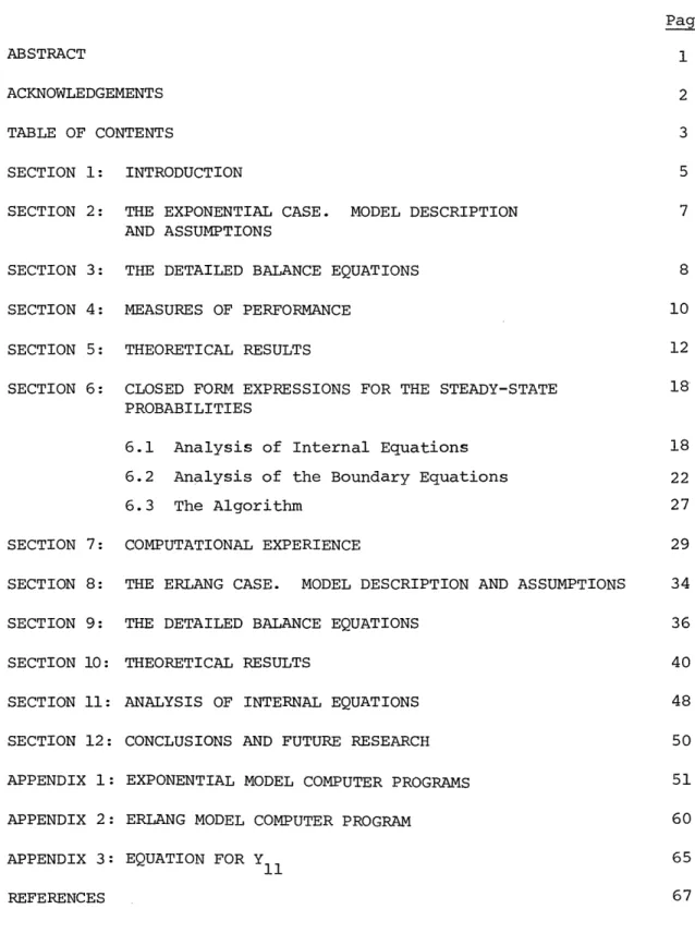
-2-Page

ABSTRACT 1

ACKNOWLEDGEMENTS 2

TABLE OF CONTENTS 3

SECTION 1: INTRODUCTION 5

SECTION 2: THE EXPONENTIAL CASE. MODEL DESCRIPTION 7 AND ASSUMPTIONS

SECTION 3: THE DETAILED BALANCE EQUATIONS 8

SECTION 4: MEASURES OF PERFORMANCE 10

SECTION 5: THEORETICAL RESULTS 12

SECTION 6: CLOSED FORM EXPRESSIONS FOR THE STEADY-STATE 18 PROBABILITIES

6.1 Analysis of Internal Equations 18 6.2 Analysis of the Boundary Equations 22

6.3 The Algorithm 27

SECTION 7: COMPUTATIONAL EXPERIENCE 29

SECTION 8: THE ERLANG CASE. MODEL DESCRIPTION AND ASSUMPTIONS 34

SECTION 9: THE DETAILED BALANCE EQUATIONS 36

SECTION 10: THEORETICAL RESULTS 40

SECTION 11: ANALYSIS OF INTERNAL EQUATIONS 48

SECTION 12: CONCLUSIONS AND FUTURE RESEARCH 50

APPENDIX 1: EXPONENTIAL MODEL COMPUTER PROGRAMS 51

APPENDIX 2: ERLANG MODEL COMPUTER PROGRAM 60

APPENDIX 3: EQUATION FOR Y1 1 65

REFERENCES 67

-3-LIST OF FIGURES

Page Figure

1 Two-Machine Transfer Line 5

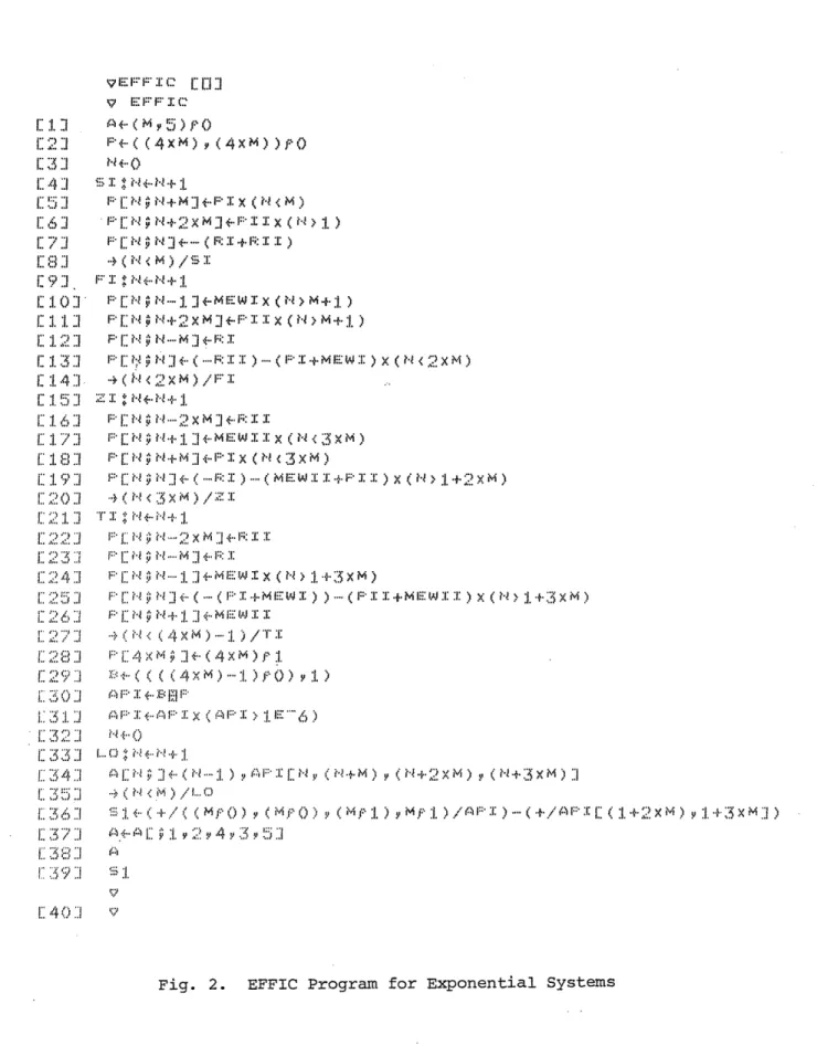
2 EFFIC Program for Exponential Systems 53

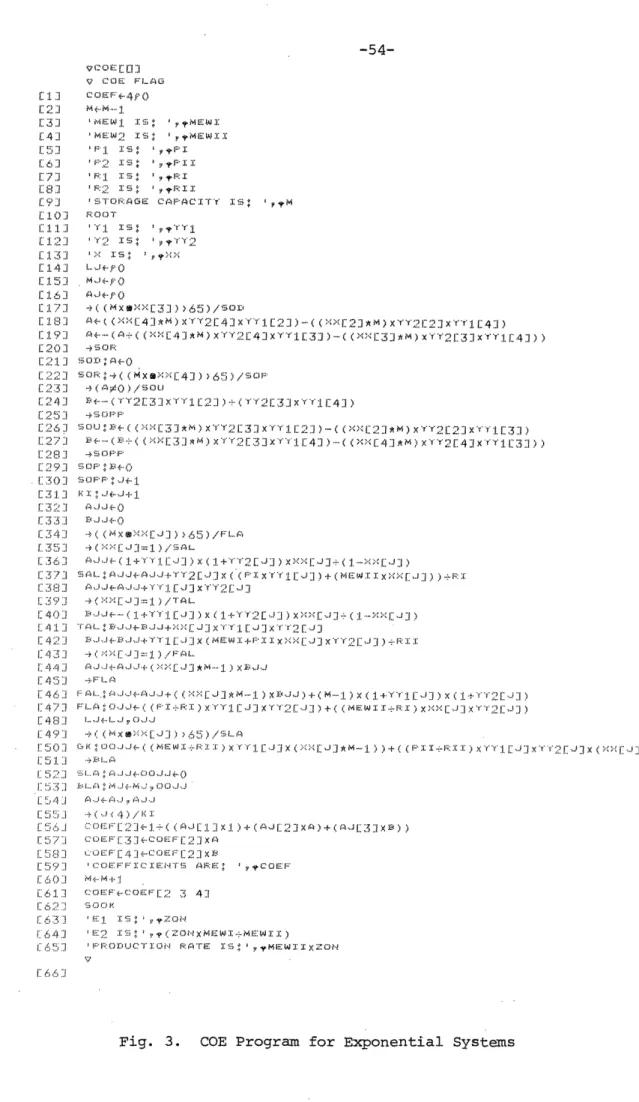
3 COE Program for Exponential Systems 54

4 ROOT and ROOT1 Programs for Exponential Systems 55

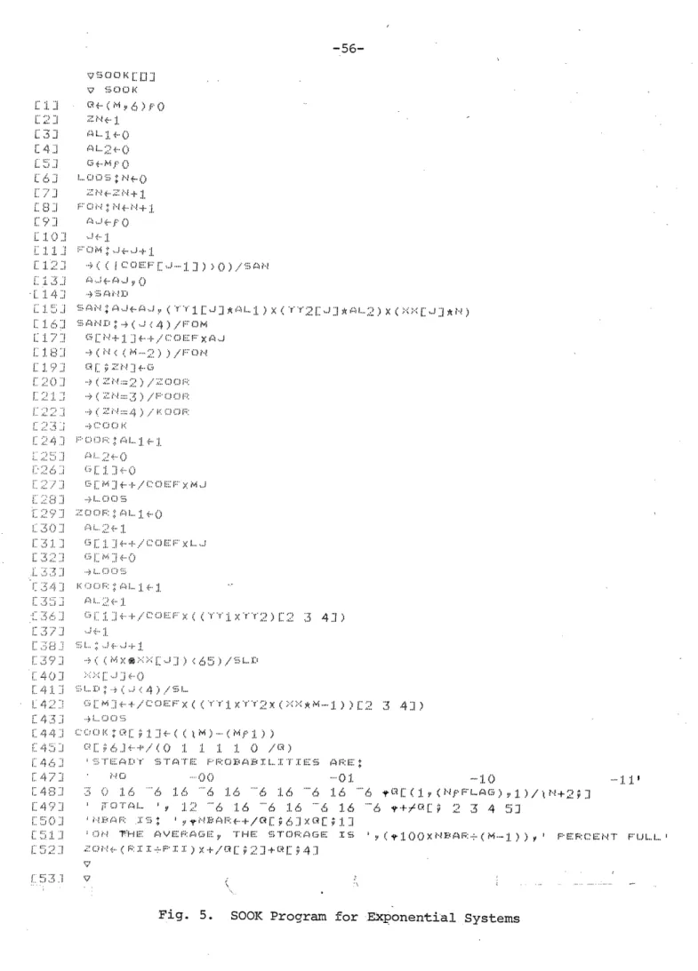
5 SOOK Program for Exponential Systems 56

6 Output of COE 1 for Exponential Systems 58 7 Output of COE 0 for Exponential Systems 59 8 EFFIC Program for Erlang Systems 62 & 63

9 Output of EFFIC for an Erlang System 64

-4-An important attribute of the components of systems is their reliability. Components may be unavailable because of routine maintenance or because of repairs for failures. For various reasons (e.g., the difficulty of diagnosing a failure), the length of time that a component is not available to perform

its intended task is a random variable.

In many kinds of systems, buffer storages are present. These buffers have the effect of decoupling the system so that changes from normal operating conditions at one part of the system have minimal effect on the operation of other parts of the system. While this is often useful, the precise effect of such storages on system-wide behavior is only partially understood.

This report is concerned with a special class of systems with storage--the two-machine flow shop or transfer line. This class is illustrated in Fig. 1. Workpieces enter the first machine and are processed. They are then stored in the buffer storage and proceed to the second machine,after which they leave the system.

Machine

Morag

achine

Fig.

1 Two-Machine Transfer Line

Systems of this form, often with more machines and storages, are found in many applications. We use the term "machine" here to describe the site where operations take place. The terms "processor", "stage", or "station" could also be used. The machines can then represent machine tools,

chemical reactors, digital computer components, etc. A survey of the literature appears in Schick and Gershwin (1978).

The research reported here is focussed on systems in which the storage is finite, the machines have random failure and repair time distributions, and the processing times of the machines are random. The failure and repair time distributions are exponential. Two kinds of processing time distributions

-5-

-6-are considered: exponential and Erlang. The results reported here differ from earlier work in the random nature of the processing times.

Two interpretations are appropriate for the assumption of random processing times. The first is that the system is intended to produce

identical parts. The raw pieces have random attributes (such as the amount of metal that must be removed). The processors also have random attributes (such as the quality or amount of wear of tools). The inter-action of these effects leads to random processing time.

The second interpretation is that the pieces to be processed are different and require different operations. For example, the pieces may be computer jobs passing through a main processor and an I/O facility.

The second interpretation is particularly significant for flexible manufacturing systems. A flexible transfer line is one in which the machines are capable of a range of operations on different pieces. These operations may take different lengths of time to perform. The

random-ness arises from the pieces, which arrive at the first machine in random sequence.

In Sections 2 through 7 we analyze systems whose machines have ex-ponentially distributed processing times. Section 2 contains a formal

description of the model and its assumptions. Section 3 is a complete statement of a Markov process representation of the system. Performance measures such as efficiency, production rate, and average in-process

inventory are described in Section 4. Section 5 contains some theoretical results on this model and Section 6 completely characterizes the steady-state probability vector. Some numerical experiments are described in Section 7.

Systems with Erlang distributed processing times are discussed in Sections 8-11. The formal description of the model is in Section 8; the Markov process is presented in Section 9; and theoretical results appear in Section 10. Here, results are not as well developed as in the ex-pontial case, and a partial characterization of the steady state prob-ability vector appears in Section 11.

Section 12 presents conclusions and outlines needed in future research. Computer programs can be found in the appendices.

The system consists of two machines that are separated by a finite storage buffer. Parts enter machine 1 from the outside. Each part is operated upon in machine 1, then passes to the buffer and then proceeds to machine 2. After being operated on in machine 2, the part leaves the system. It is assumed that a large reservoir of parts is available to machine 1.

Figure 1 shows such a system. Each machine can be in two possible states

-operational or under repair. Only when a machine is -operational can it

perform operations. There are, however, conditions on the storage buffer

under which a machine can not operate, even if it is in the operational state.

If the storage is full there is no place for parts from machine 1 to go.

If the storage is empty there are no pieces available for machine 2 to

oper-ate on.

A machine can fail only while it operates on a piece.

Service, failure and repair times for machine i are assumed to be

expo-nential random variables with parameters pi' Pi, ri; i=1,2 respectively.

The capacity of the storage buffer in N units. We define a binary variable

ai to represent the state of machine i. If ai=l, machine i is operational

and if a.=0, machine i is under repair.

Let n denote the number of units in

the storage plus the number of units in machine 2 (which can be zero or one).

Then 0 < n < N+1.

In the next section we characterize the steady state balance equations.

These steady state probabilities are essential for computing system

perform-ance measures such as efficiency, production rate,and average in-process

inventory.

-7-3. THE DETAILED BALANCE EQUATIONS

Let the state of the system be represented by

s= (n,al, a2)

with n=0,1,...,N; ai=0,1; i=1,2. Whenever n=O, machine 2 cannot operate on a piece, and whenever n=N, machine 1 cannot operate on a piece.

We distinguish four sets of detailed balance equations, corresponding to the values of a1 and a2. For a1=a2=0 we have

p(n,O,O) (rl+r2) = p(n,l,0)p1 + p(n,0,l)p2, l<n<N-l (3.1)

p(0,O,O) (r1+r2) = p(O,l,0)pl (3.2)

p(N,0,0) (rl+r2 ) = p(N,0,l)p2 (3.3)

This reflects the fact that the system leaves state (n,0,0) only if repair of one of the two machines takes place. We can reach state

(n,0,0) either from state (n,l,0) (unless n=N) if machine 1 fails or from state (n,0,1) (unless n=O) if machine 2 fails.

The other three sets of equations can be explained in a similar way.

O1=0, a2=1:

(3.4) p(n,0,1) (rl+p2+p2) = p(n,0,0)r2 + p(n,l,l)p1 + p(n+l,0,1)12, l<n<N-l p(0,0,1)rl = p(0,0,0)r2 + p(0,l,l)p1 + p(l,0,l)p2 (3,5) p(N,0,l)(rl+P2+p2) = p(N,0,0)r2 C3.6) al=l, a2=0: p(n,l,0) (pl+11+r 2) = p(n-l,l,O)p1 + p(n,0,O)r1 + p(n,l,l)p2, (3.7) l<n<N-1

-8-p(,l,0) (pl+Pl+r 2) = p(0,0,O)rl (3.8)

p(N,1,0)r₂ = p(N-l,l,0)p1 + p(N,0,0)rl + p(N,l,l)p2 (3.9)

a1=1, a 2=1:

p(n,l,1) (p +p2

+1l+

)

=

p(n-l,l,l)l1 + p(n+l,l,l)'p

+

(3.10)

+ p(n,1,0)r2 + p(n,0,1)r , l<n<N-1

p(Ol,l)

(pl+ l) = p(l,l,1)p2 + p(O,l,0)r

2

+ p(O,0,1)rl

(3.11)

p(N,l,l) (p

2

+P

2

) = p(N-1,1,1)

1

+ p(N,l,0)r

2

+ p(N,0,l)r

1

(3.12)

In Appendix 1 we present a computer program in the APL language

for solving the detailed balance equations. The total number of these

linear equations is (2 )(N+1) so that when N is large this becomes

costly. In Section 6 we present a more efficient method of finding the

steady state probabilities. In the next section we discuss measures of

performance, and in Section 5 we derive some theoretical results based

4. MEASURES OF PERFORMANCE

There are three measures of performance that are often used as criteria to evaluate the performance of production systems.

The first measure of performance is the efficiency E. of the i'th machine in the system. Efficiency E. is defined as the probability that the i'th machine is operating on a piece, or the fraction of time in which the i'th machine produces pieces. We can express the efficiencies in terms of the steady state probabilities as:

N-1 1 E1 E

E

p(nl'a2) (4.1) 1-20 a2=0 N 1 E2

=E

V'

p(n, l,l)

(4.2)

n 1

lo

1

It is important to distinguish Ei, the efficiency of the i'th machine in the system from ei (defined in equation (6.53)),the efficiency of

machine i if it were operated in isolation. The former is affected by the other machines and the storage while the latter is a characteristic of machine i only.

In Lemma 5 in the next section we show that

P1E, = P2E2 . (4.3)

The quantity .iEi can be interpreted as the rate at which pieces emerge from machine i. Equation (4.3) is then a conservation of flow law, and we can define

P = i.E. . (4.4)

This is the production rate of the system.

The efficiency E of the system is defined as

actual production rate

production rate in the absence of failures

-10-Since 1/pi is the average time a piece spends in machine i when no failure

takes place, pi is the production rate of machine i in isolation in the

absence of failures.

The production rate of the system without failures

is thus less than min(pl,]1

) 2

and E satisfies

E > (4.6)

-- min(lpl'lJ 2)

Assume i = min(pl,p

₂

).

Then from (4.4),

E >E.

Note also that if Vi < pj (i,j = 1 or 2, ifj) then (4.3) implies

that E. > E..

Therefore, the system's efficiency satisfies

-

J

E > max(EE 2 (4.7)

Another important measure of system performance is the expected

in-process inventory.

This can be written

N 1 1

n = E E

2

np(n,al,a2o

.

(4.8)

n=O a = a =0

5. THEORETICAL RESULTS

In this section we derive some theoretical results. These results are important in providing insight into the model as well as a basis for our discussions in the following sections.

In the first lemma we prove that some of the steady state probabilities are zero.

Lemma 1

p(O,O,O) = p(Q,1,0) = p(N,O,O) = p(N,O,l) O0 (5.1)

Proof: Combining equations (3.2) and (3.8) yields:

p(0,0,0)r2 + p(0,1,0) (P l+r2) = 0 (5.2)

Since probabilities are non-negative, p(0,0,0) = p(0,1,0) = 0. Combining equations (3.3) and (3.6) yields:

p(N,0,0) rl = p(N,0,1)(rl') 2 = 0 (5.3)

Similarly, this implies that p(N,0,0) = p(N,0,1) = 0.

Lemma 2 asserts that the rate of transitions from the set of states in which machine 2 is under repair to the set of states in which machine 2

is operational is equal to the rate of transitions in the opposite direction.

Lemma 2

N 1 N 1

r2

EP2

p(n, = p2 ,l) (5.4)

n=O a1=O n=l a1=0

probability that machine probability that machine 2 2 is under repair can operate

-12-Proof

Add equations (3.1)-(3.3) and (3.7) - (3.9):

N N-1 p(n,O,O) (r +r₂) + p(n,l,O) (Pl+l +r2) + r+ 2p(N,1,0) n=O n=O N-1 N N =P 1 P p(n,l,O) + P2 1 p(n,O,1) + Vp1 I p(n-l,1,0) + n=O n=l n=l N N r1 Z p(n,O,O) + P2 7 p(n,l,1) (5.5) n=O n=l

This can be reduced to

N N N

r2

>

p(n,O,O) + r2

>

p(n,l,O) = P2

>

p(n,O,1) + (5.6)

n=O n=O n=l

N

P2 1 p(n,l,l) n=l

which is equivalent to equation (5.4)

Lemma 3 establishes a corresponding result for machine 1.

Lemma 3

N 1 N-1 1

nr1

7

p(n,'0 ) 2 P1 n

>

p(n,l,c 2) (5.7)

n=0 a2 n=O a2=O

Probability that Probability that Machine 1 is under Machine 1 can

repair operate Proof Add equations (3.1)- (3.6): N N n p(n,o,O)(rl+r2 p(nOl)( ₂2l+r++p2) + n=+ p(OOl)rl + p(0,0,1)r1

-14-N-1 N

= P1 n p(n,l,0) + P2 n p(n,0,1)

N N-1 N-1

+ r2 np(n,,0) + p1 + 1=2 p(n+l,)0,) (5.8)

This can be reduced to

pnOON N N-1 N-1

rl n _ p(n,0,0) +rl n p(n,0,l) = Pn 1 p(n,l,0)+ P1 n p(n,l,l)

(5.9)

which is equivalent to (5.7).

Lemma 4 shows that the rate of transitions from the set of states with n pieces in storage and machine 1 operational to the set of states with n+l pieces in storage and machine 2 operational is equal to the rate of transitions in the opposite direction.

Lemma 4

1 1

111 0 p(n,l,a2) = 12 E p(n+l,'all), 0<n<N-1 (5.10)

Probability that Probability that Machine 2 machine 1 is opera- is operational with n+l tional with n pieces pieces in storage

in storage.

Proof: By induction.

For n=0, add equations (3.2), (3.5), (3.8) and (3.11). Using the results of Lemma 1 we get

p(0, ,l)r1 +p(,0,l,l)p 1 + p(p(0,1)l) 2 (5.11)

or

p(0,1,1)I1 = p(l,0,l1) 2 + p(l,l,l)P 2 . (5.12)

Since p(0,1,0)= 0 this is equivalent to

1 1

P

E

P(0,1,a

22=

)

P2

p(l,

1 1

1)

(5.13)

a2=0 a, =0

which is equation (5.10) with n=0.

Let us assume that equation (5.10) holds for n=m<N-2. We show that this

implies (5.10) for n=m+l. Add equations (3.1), (3.4), (3.7), and (3.10)

with n = m+l (1 < m+l < N-l).

This yields

p(m+l,0,0) (rl+r

2

) + p(m+l,l,0)(pl+P1+r

)

2

+

+ p(m+l,0,1)(rl+1

2+P

2

) + p(m+l,l,1)

(p

1

+p

+ P

2 1

+2)

=

p(m+ll,)p

+

p(m+l, O,l)p! + p(m+l,

₂

,1)

+ p(m+l,0,0)r

1 + p(m+l,l,l1)p 2 + p(m+l,0,0)r2 + p(m+1l,l,)pl + + p(m+2,0,1) 12 + p(m,l,l)11 + p(m+2,1,1)112 + p(m+l,l,0)r2

+ p(m+l,0,1)rl

(5.14)

This can be reduced to

p(m+l,l,0)p1 + p(m+l,0,1)1

2

+ p(m+l,l,l) (p1+2

)

-16-But by induction

p(m,l,0)p1 + p(m,l,l)pl = p(m+l,0,1)p2 + p(m+l,l,l)p2 (5.16)

and therefore (5.15) becomes

1 1

P₁

Y

p(m+l,l,' 2) = 2 E p(m+2,all) (5.17)

a2=0aU0 1

Therefore, equation (5.10) holds for 0<n<N-2. To prove the lemma for

n=N-l add equations (3.3), (3.6), (3.9), and (3.12) to yield , with Lemma 1,

p(N,1,0)r2 + p(N-l,l)(p+i2 2) = p(N-l,l,0)~1 + p(N,l,l)p2 + p(N-l,l,l)111 + p(N,l,0)r2 (5.18) or p(N,L,1)p₂ = p(N-l,1,0o) 1 + p(N-1,l,l)p 1 (5.19) or 1 1 P1

p(N-ll

2) =

(N,al)

(5.20)

since p(N,0,1) = 0. This is equation (5.10) for n=N-1, so the lemma is proven.

In the next lemma we prove that the rate of transitions between the set of states in which machine 1 can produce a piece and the set of states in which machine 2 can produce a piece are equal.

Lemma 5

N-1 1 N 1

'1 p(n,l,a2) = 2n E1E p(n,a111) (5.21)

Probability that Machine Probability that Machine 1 c&i produce a piece 2 can produce a piece

Proof: Equation (5.21) is simply equation (5.10) summed for n= 0,...,N-1. This lemma is interpreted in Section 4.

6. CLOSED FORM EXPRESSIONS FOR THE STEADY STATE PROBABILITIES 6.1 Analysis of Internal Equations

We define internal states as states (n,1 ,2 ) where l<n<N-l.*

1 2

--Internal equations are the detailed balance equations that do not include any boundary states. The rest are called boundary equations. Following the analysis in Schick and Gershwin (1978) we guess a solution

for the internal equations of the form

n

a a2

p(n,al,a 2 )= cX Y1 Y2 l<n<N-l (6.1)

where c,X,Y ,Y₂ are parameters to be determined.

By substituting(6.1) into the internal equations we find that those equations are satisifed if X,Y₁,Y ₂ satisfy the following three non-linear equations: PlY1 + P2Y2 - r1 - r2 = 0 (6.2)

1

rr

1x

_

1

1

=

p1(-

- 1) - PlY

1 +

r

1 +

Y-

1

0

(6.3)

r2 p2(X- 1) - P2Y2 + Y + rP2 - 2 = 0 (6.4)

This is because the internal equations (equations (3.1), (3.4), (3.7), and (3.10)) can be written

*This is in contrast to the deterministic processing time case (Schick and Gershwin, 1978) in which the internal states are those in which 2<n<N-2.

-18-l 1 1-2 2 p(n,cl, '2) (rl P1 + r2 P2 = (p(n-l,cl,o2) - p(n,al,C2) )Pw1 + (p(n+l,0₁,c2) - P(n,al1,2)2a 2 51 11-e + P(nl-

1l'a

2)rl P1

a

₂

1-52

oc2 l-l2

+ P(n,a 'l-ca

2

)r

2

P

2

(6.5)

If p(n, l,a2) is given by (6.1), equation (6.5) becomes

n 51 a2

1-51 a1

1- 2 a2

X Y Y2 (r p1 + r P

n

a

a

2 1 "p2 r ₁ YY 1Y(X-l) = X Y1 Y2 ll ( X -1) + X Y1 2 2(X-1) n 1- _1-2 2 al 11-a n al ₁₂ 1- ₅₂ 2 1-a 2

+

X Y Y rl P - X Y Y r2 P2 (6.6)

1

2

1

1

1

2

2 2

or

1- 1 a1

1-52 a2

rl P1 + r2 P2 P1 1( - 1) + p2a2(X-1)

1-2a₁ aI 1-a1 1-2a2 a2 1-a2

+ Y1

rl P1

+ Y

2

p2

_(6.7)

or, finally,

1

1-2a1 a

₁

1-a

₁

1-a5

1

a

0 = {1 (-- 1) + Y _{1 -P rl}

1-2a2

a

1-a2

1-c 2 a2

-20-Equation (6.2) follows when a1= a2 = . Equation (6.3) and (6.4) result from aL= 1, a2 = 0 and a1= 0, a2 = , respectively. When a1=, 2 = 1,

the result is the sum of equation (6.3) and (6.4). This development holds for lines of -k machines and k-l storages, although the boundary behavior has not yet been investigated.

Equations (6.2)-(6.4) can be reduced to the -following fourth degree polynomial in Y1: 34 2 2 2 2 2 3 3 P1

Y

1 + (-p2P1 3Prl - p1

r

2 - P2P1 +

VIP1

+ P1)Yi 2 2 + (2p2Plrl - r2Pl P1 - 2rlPl B1 - P2Pll P - P2P1 - 3Plrl 2 2 2 - Plr2 - P2P1 + 2rPl 2 + 3Plrl + 2Plrlr2 + 2PlP2rl) 1 + (2P1P 2r1 + rlrl rlr2 + rr2plr1p1 2 + 212 + 1P2 2 2 2 3 + 3pr 1 + 1 2rr2P1 - 2r - rlr2

}

2 - rlP2 - r1 2 2 3 2 -rlr₂)Y₁ + (-r_{1 2} (rl+r2) - rlr2 - rl - rlP2) =

0

(6.9)

It is easy to verify that one solution is

r₁

-- 11

-p(6.10) p1

and by substituting (6.10) in (6.2) and (6.3) we obtain:

r2 2 and

X₁ =1 (6.12)

The other three solutions to (6.9)can be obtained by solving a cubic

equation. We can write (6.9) as

Pl(plY1- r) (Y

₁

+ 3sY

₁

+ tY

₁

+ u) =

(6.13)

where s, t and

u

are given:

by

1 3s = (-

2r

1 - r2 - P2 + 1 + P) (6.14)

t -

2

(

12rl

r2~l

-

-

rlpl

-2P

P2B1

P1

2

-2Plr - Plr2 - pP2 + 12r2 + rl

1

1

1 2

1 2

22

1

+ rlr

₂

+ rlp

2 )

(6.15)

2 ( (rl+r2)

+

rl

+

2

rl

+

r2 )

(6.16)

P1

The other three values for Y1 are (Chemical Rubber, 1959)

Y12 = 2

-

cos

(

6.17)

Y13 = 2/ 3 cos

(3

+ 21T/3)

(.6.18)

13 3 Y = 2- - cos ( + 47/3) (6.19)

where:

a

= - (3t - s2) (6.20)

3

-22-1

2

b = (2s - 9st + 27u) (6.21)

and

= arcsinl i

2

(6.22)

Again Y2i, X

i

for i = 2,3,4 can be obtained from (6.2)

and (6.3).

The conclusion is that for the internal equations:

Y a D

p(n,ala2) = Cj Xn Yl 22 c(6.23)

j=l

lj

2j

where c., j= 1,2,3,4, are parameters to be determined.

6.2 Analysis of the Boundary Equations

There are a total of eight boundary states.

The probabilities of

four of them are specified by Lemma 1. The other four are characterized

in the next lemma.

Lemma 6

p(O,O,1)

= cj

(P

1

YljY

2 +

v2XY2j

Y) (6.24)

4

p(O,1,1) = ~C.jYljY2j (6.25)

4.

CJ

= (clXlj + P2XjYljY2j (6.26)

p(N,1,0)

E=Cr

=

+ (6 26)

4

p(N1,l1) = c.XYj Y (6.27)

j=l j lj 2j

Note that (6.25) and (6.26) are in the internal (6.23) form. Further-more, the coefficients c. satisfy

c = 0 (6.28) 4 E

cjYj

= 0 (6.29) j=2 4 E cjX y2j = 0 (6.30)

and the normalization equation,

N 1 1

E

E

E P(nlal

a2

) = 1 (6.31)

n=0 a=0 a 2=0

Proof: The expressions (6.23) - (6.27) and (5.1) satisfy all the detailed balance equations (3.1)-(3.12) identically except for the following.

Equation (3.11) becomes

4

0 = cjY2j(PlYlj P2XjYlj X) . (6.32)

j=l 2j

Equation (3.7), for n= 1, becomes

4

0 =

L

cjXj [P

1+P1+r2)Yl P2Yljy2j] - r1 - (6.33)

-24-Equation (3.12) becomes

4 N-i

0 = c.X. Yj(2XjY2j - 1Y2j - 1) (634

j=l 3 3

and equation (3.4), for n = N-1, is

4

0 = c.X. [(r2 +P-pY2j r2 P1 Yl y] (6.35)

j-1 J

1 2 2 2j

2

1

i

2j

Equation (6.33) can be transformed by observing that

(p1

+1

+r2)Ylj - r1 - PYljY2j

= (P1Ylj- rl) + p1Ylj + Ylj (r 2-P2Y2j) (6.36)

= (p Ylj - r)Y (r1 -p )+Yi) (6.37)

(because of equation (6.2)), and finally,

= (P1Ylj - rl)((lj) +

)+IYlj (6.38)

Note that equation (6.3) can be written

- 1) = (P Y - r )

-

(6.39)

1 .

1

lj -I.

so that expression (6.38) is

p1(X) 1)Ylj + Y lj /Xj (6.40)

4

o

= j

c

jY lj

'

(6.41)

j=_

The same sequence of steps can be applied to equation (6.35) to yield

4

o

=

CjXY2j

(6.42)

j-l c

j

2j

To analyze (6.32), we first observe that equation (6.39) implies

P1Y lj - 2Xj(Ylj+l) =

21 l)lj

Pl Yj

2

P lj rl (6.43)

if P1Ylj -rl / 0. Recall that

P1 Y -r = 0

Equation (6.4) can be written

(i+Y 2j

2(Xj- 1) = (P2Y2j - r2j) (6.44)

2 r 22j 2j Y2j

so that (6.43) can be transformed to

-lYlj/Y2j ' (6.45)

with the use of (6.2),still assuming PlYlj- r1 3 0. Equation (6.32) can

now be written

0 = C1Y2 1(P1Y1 1- 2X1Y1 1- 12X1)

4

-l

c

Yi

lj

(6.46)

-26-or, using (6.10) - (6.12),

r2

rl ri 4

2 1 4

-l2

=

2 p

1

2)

1 jP2

i

lj

(6.47)

Finally, we observe that (6.29) implies that

4 r1

4 cjj

p

(6.48)

j=2

l

1

so that (6.47) can be written, after some transformation, as

0=

c

I

r22

(6.49)

By the same sort of manipulations, equation (6.34) can also be transformed

into equation (6.49).

To complete the lemma, two cases must be considered.

If

!llr₁ P2r2

-- ¢ 2 (C6.50)

rl+P 1 r2+p2

then (6.28) follows from (6.49); and (6.29) and (6.30) follow from (6.28),

(6.41)

and (6.42).

If

lr

1

r

₂ 2 (6.51)

rl+P 1 2+P2

then cl is not determined by (6.49). However, in this case Y

1

= r /Pl is

(6.17) - (6.19) (j = 2,3,4) is rl/Pl. Then there are only three

in-dependent sets of parameters (Xj,Ylj,Y2j) and the coefficients c. are

given by (6.29) - (6.31).

As a final note, the values of c

₂

, c

3

and c

4

can also be found by

solving (5.3) and (5.6) and the normalization equation (6.31).

The quantities

1.r.

1 1

i

r.+Pi

_{1 1}

(6.52)

that appear in equation (6.49) have physical significance. We define

Pi as the isolated production rate of machine i, the production rate it

would have if it were not part of a system with other machines and

storages. The ratio

r.

e. =

(6.53)

ri +Pi

in the fraction of time it is available (i.e., not under repair) if it

were in isolation. This quantity is the isolated efficiency. Since

pi is the production rate while machine i is operational,

.iei

is the

production rate in isolation.

6.3 The Algorithm

Now we can find all the steady state probabilities of the system

using the following algorithm:

Step 1

-28-Step 2

Solve equations (6.29)- (6.31) to obtain cj; j=2,3,4.

Step 3

Use Lemma 1 and equations (6.23) - (6.27) to evaluate all probabili-ties. These probabilities can be used to evaluate the measures of

In this section, we describe the results of a set of numerical ex-periments with the model described above.

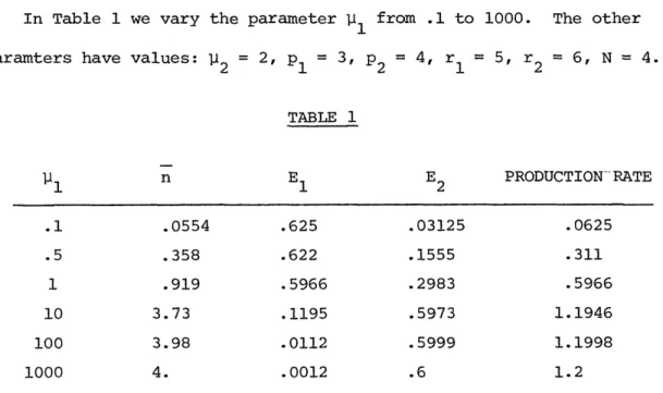
In Table 1 we vary the parameter p1l from .1 to 1000. The other paramters have values: p2 = 2, P1 = 3, P2 = 4, r1 5, r2 6, N = 4.

TABLE 1 n E1 E2 PRODUCTION--RATE .1 .0554 .625 .03125 .0625 .5 .358 .622 .1555 .311 1 .919 .5966 .2983 .5966 10 3.73 .1195 .5973 1.1946 100 3.98 .0112 .5999 1.1998 1000 4. .0012 .6 1.2

We see that as 1pi1 the rate of service for machine 1 increases, both

E2 and the production rate increase to a limit of .6 and 1.2 respectively.

That is, there is a saturation effect, and no amount of increase in the speed of machine 1 can improve the productivity of the system. Note that as the first machine is speeded up, the amount of material in the storage increases. This is the reason for the increase in production rate.

In Table 2 we vary the parameter p2 from .1 to 1000 for the case

= 1, p = 3, P2 = 4, r1 5, r2 = 6, N = 4.

-29-

-30-TABLE 2 n E1 E2 PRODUCTION RATE .1 3.89 .0599 .59990 .0599 ,5 3.19 .2903 .5806 .2903 1 2.08 .4836 .4836 .4836 10 .124 .62471 .06247 .6247 100 .0111 .6249 .006249 .6249 1000 .00109 .625 .000625 .625

In this case we see that although E2 decreases, the production rate

increases as p2 increases. When the second machine is very fast, it frequently empties the storage and thus spends a lot of time starved for pieces. Consequently E2, the fraction of time machine 2 is operating

on a piece, is small. The production rate, in the limit as p2 is large, is simply the isolated production rate of the first machine,

Plrl/(rl+pP). Here as p2 increases, the number of pieces in storage decreases.

These two tables lead to the following tentative conclusion: If all other things are equal, it is better to speed up downstream machines than to speed up upstream machines. Both can increase over all

production rate, but if downstream machines are made faster, the average in-process inventory is reduced.

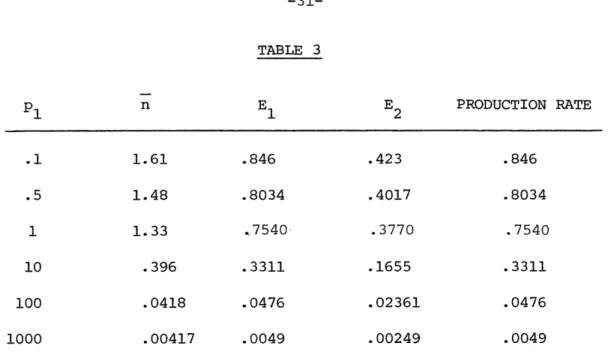
In Table 3 we vary the parameter plfrom .1 to 1000 for the case:

TABLE 3 P1 n E1 E2 PRODUCTION RATE .1 1.61 .846 .423 .846 .5 1.48 .8034 .4017 .8034 1 1.33 .7540 .3770 .7540 10 .396 .3311 .1655 .3311 100 .0418 .0476 .02361 .0476 1000 .00417 .0049 .00249 .0049

As the rate of failure of the first machine increases, the average in-process inventory, production rate, and the efficiencies E1 and E2

go to zero together.

In Table 4 we vary the parameter P2 from .1 to 1000 for the case

=

,

2 =

2,

p₁ = 3, rl = 5, r2 = 6, N = 4. TABLE 4 P2 n E1 E2 PRODUCTION RATE .1 .464 .6194, .3097 .6194 .5 .507 .6174 .3087 .6174 1 .562 .6158 .3079 .6158 10 1.66 .5322 .2661 .5322 100 3.77 .1131 .0565 .1131 1000 3.98 .0119 .0060 .0119

Again as the rate of failure for the second machine increases, E1, E2, and the production rate approach zero, but here n approaches

-32-In Table 5 we vary the parameter value rl from .1 to 1000 for the

case 1, 2 = 2, p = 3, p2 4, r2 = 6, N = 4. TABLE 5 r1 n E1 E2 PRODUCTION RATE .1 .0342 .03225 .01612 .03225 .5 .161 .1426 .07128 .1426 1 .300 .2486 .1243 .248.6 10 1.20 .7104 .3552 .7104 100 1.59 .8411 .4206 .8411 1000 1.64 .8554 .4277 .8554

As the rate of repair for the first machine increases, E1, E2,

n, and the production rate increase. Note that n does not approach N= 4.

In Table 6 we vary the parameter value r2 from .1 to 1000 for the

system pi= 1, p2 = 2, P1 3, p2 = 4, r 5, N = 4. TABLE 6 r2 n E1 E2 PRODUCTION RATE .1 3.88 .0486 .02431 .0486 .5 3.36 .2144 .1072 .2144 1 2.74 .3575 .1787 .3575 10 .720 .6088 .3044 .6088 100 .477 .6191 .3095 .6191 1000 .455 .6198 .3099 .6198

Again when the rate of repair for the second machine increases, both the efficiency E2 and the production rate increase. The

in-process inventory decreases.

In Table 7 we vary N from 2 to 100, for the transfer line pi = 1,

2= 2, p = 3, P2 4, r₁ = 5, r₁ = 5, r2 = 6. TABLE 7 N n E1 E2 PRODUCTION RATE 2 .599 .5228 .2614 .5228 5 1.01 .6093 .3047 .6093 10 1.16 .6242- .3121 .6242 20 1.18 .625 .3125 .625 50 1.18 .625 .3125 .625 100 1.18 .625 .3125 .625

We see from the table that as N increases, both the efficiencies and the production rate increase up to a limit. This case seems to display the same saturation effect as in Table 1. Furthermore, the average in-process inventory also approaches a limit as the buffer capacity increases.

These examples are not intended to be exhaustive. They are furnished to show the kind of result that is obtainable with this model, and that its behavior agrees with intuition.

8. THE ERLANG CASE. MODEL DESCRIPTION AND ASSUMPTIONS

Until now we have restricted our discussion to a particular service time distribution - the exponential. This assumption however, may be-come quite troublesome for many systems. -In order to have a more realistic model we must allow a more general service time distribution.

In this model we assume that the service time distribution for the two machine is Erlang with K(K> 1) phases.* The advantage of this assumption is that a very large class of distributions can be approxi-mated very closely by Erlang distributions (Kleinrock, 1975).

A consequence of the new service time distribution assumption is that we can now find each of the two machines in K+l states, since in addition to being under repair the machines also can be operational

in any one of the K phases of the Erlang distribution.

Let i and j represent the states of each of the two machines,

i, j = 0,1,..., K. By i= 0 we mean that machine 1 is under repair and

by i = m (1< m < K) we mean that machine is operational and ready th

to start the m

Erlangian phase.

Again we assume that machine 1 can operate on a piece only if it is operational and n< N. Machine 2 can operate on a piece only if it is operational and n>O. We also assume that when a machine fails the piece that was being processed when the machine failed must start its service from the beginning, that is from the first phase.

We consider the system in steady state. Due to the Erlang distri-bution assumption we have a Markovian model.

The quantities ri, Pi and N have the same meaning as in the

ex-ponential case. This implies that the rates of failure and repair are *Also known as the gamma distribution, with integer shape parameter.

-34-independent of what phase the system was in when the last failure

occurred. However, pi is now the rate that machine i completes each 1

of its Erlangian phases. Thus, the production rate of machine i,

9. THE DETAILED BALANCE EQUATIONS

Again we denote (n,i,j) to be the state of the system; n= 0, 1,...N; i,j = 0 , 1,2,..., K, K > 1. By our assumptions machine 2 cannot operate on a piece unless n> Q. Therefore, the probability of any state with n= 0 and j> 1 or n=N and i > 1 is zero. That is,

p(0,i,j) = 0, j = 2,..., K , i = 0,,...,K (9.1)

p(N,i,j) = 0, i = 2,..., K , j = 0,1,...,K (9.2)

Again we distinguish between four sets of detailed balance equations, to correspond to the values of i and j.

For i= j =0 we have K K p(n,0,0) (r +r) 2= p(n,i,0)p + Z p(n,0,j)p₂ , l<n<N-1 (9.3) 12 i=l 1 j=1 K p(0,0,0) (rl+r2) = p(0,i,0)p1 (9.4) i=l K p(N,0,0) (rl+r2) = Z p(N,0,j)p2 (9.5) j=l

These equations represent the fact that the system enters state (n,0,0) either from state (n,i,O) (n7N, i70) if machine 1 fails or from state (n,O,j) (n/0, j3O) if machine 2 fails.

For i = 0, j o0, K p(n,0,j)(r 1+12+ 2) = p(n,0,j-1)p2 + Z p(n,i,j)pl , (9.6) te.~

~

i=1 2 < j < K, 1 < n < N-1

-36-K p (n,0,1) (r +2+P2) = p(n+l,0,K)p2 + Z p(n,i,l)p + p(n,0,0)r2 (9.7)

1 22

2

1

2

i= 1 < n < N-1 K

p(0,0,1)r1 = p(1,O,K)j2 + Z p(0,i,1)p + p(O,0,O)r2 (9.8)

i=l

p(N,0,j) (rl+ 2+P 2) = p(N,0,j-1)1 2, 2 < j <k (9.9)

p(N,O,1) (rl+pJ2+p2 ) = p(N,,O)r2 (9.10)

For j= 0, i 3 O,

K

p(n,i,O) (pl+pl+r2) = p(n, i-1,0)p + Z p(n,i,j)p2, (9.11)

j=1

2 < i < K, 1 < n < N-1 K p(n,1,0) (p1+ll +r2) = p(n-1,K,0)p1 + Z p(n, i,j)p 2 + p(n,0,0)r1, (9.12)

j=1

1 < n < N-1 p(0, i, 0) (p1+ 1+r2) = p(0,i-l,O)pl1 , 2 < i < K (9.13) p(0,1,0) (pl+lll+r2) = p(0,0,O)rl (9.14) K p(N,1,0)r2 = p(N-1,K,O)pl + Z p(N,l,j)p2 + p(N,0,0)rl (9.15) j=l For i S 0, j

O0,

p(n, i,j)(p1+P2+1l 1+P2) = p(n, i-l,j)p1 + p(ni,j-1)l, (9.16)

-38-p(n,l,j) (p+p2+1 -l+-2) = p(n-1,K,j)p 1 + pmlj-1) 2 (9.17)

+ p(n,O,j)r₁ , 2 < j < K, 1 < n < N-1

p~n,i,1) (P1+P2+1+2) = p(n,i-l,l)11 + p(n+l, i,K) 2 , (9.18)

+ p(n,i, 0)r2 , 2 < i < K, 1 < n < N-1

p(n,l,1) (P1+P2+p+ 1 2) = p(n-1,K,1)p1 + p(n+l, 2,K) 2 (9.19)

+ p(n,0,1)r + p(n,l,0)r₂ , 1 < n < N-1

p(0, i,1)(pl+pl) = p(O,i-l,)1p + p(l, i,K)p 2 + p(0,i,0)r2 (9.20)

2 < i<K p(0,1, 1(pl l) = p(l,1,K)p₂ + p(0,0,l)r1 + p(O,1l,0)r2 (9.21) p(N,l,j) (p2+1 2) = p(N-1,K,j)p1 + p(N,l,j-1)p2 + p(N,O,j)rl, (9.22) 2 < j < K p(N,i,1) (p2+p2) = p(N-1,K,1)p1 + p(N,0,l)r1 + p(N,1,0)r2 (9.23) for i = 1; j = 1; n = N

Note that equations (9.14) and (9.20) imply that if the storage is. full, the first machine is not allowed to operate on pieces even

if it is operational. That is, we do not merely assume that an operation cannot be completed; we assume that an operation cannot be commenced.

In Appendix 2 we present a computer program in the APL computer language for solving all the detailed balance equations. The total

number of these equations is N(K+l) -2K

+

3.

When-either N or

K are large the computational effort becomes very great.

In Section 11

we present some preliminary work aimed at devising an efficient algorithm

for obtaining the steady state probabilities, similar to that described

above for the exponential case.

In the next section we derive some

10. THEORETICAL RESULTS

In this section we derive some theoretical results based on the detailed balance equations. These results help us to gain more under-standing of the system.

In the following lemma we prove that some of the steady state probabilities are zero.

Lemma 7

P(O,i,O) = p(N,O,j) = 0 for all i and j (10.1)

Proof: Equation (9.12) and (9.13) imply

i-1

1 or

, , ) r + r +r + p(0,0,0) (10.2)

p l+l+r2 P1 1 l++r2 Equation (9.4) can then be written

Similarly,

p(0,0,O O) (r l+r2)= p(0,0,-40- (10.3)

or

Pr(Or, 0,0) 2 + r 12 + r2 + p 1r P r0 (0.4 P1r 2

This implies that p(0,0,0) = 0 and (9.22i implies that p(0,i,0) = 0.

p(N,O,j) l 2 p(N,0,0), j = 1,..., K (10.5) 2+1 P2+P2

from (9.9) and- (9.10). Equation (9.5) can be written

r2p2 K 2 p(N,0,0)(rl+r2 ) = p(N,0,0) r 2 l 2 (10..6) 1+ 2+P2 j=l 12+P2 or p(N,0,0) 2 rl+ 2 l+rlP 2+rlr2+r2P2 r +p +

)=

0 (10.7)

and (10.1) follows as before.

Lemmas 8 and 9 establish results which are analogous to Lemmas 2 and 3 above. Lemma 8 N K N K K

r

2 E E p(n,i,0)

=

P2 E ~ p(n,i,j) (10.8) n=0 i=0 n=l i=0 j=l

probability that probability that machine machine 2 is under 2 can operate on a piece repair

Proof

Let us add equations (9.3) - (9.5) and (9.11) - (9.15).

N N-1 K p(n,0,0)(r +r2

)

+ E p(n,i,0) (P+l+r2 ) + P(N,lO)r (10.9)

1 2

1 1

2)

P

'

2 (10.9)

n=0 n=0 i=l N-1 K N K ''

=

p(n,i,O)P1 + E

L

P(n,0,j)p2

n=0 i=l

n=l j=l

N-2

K

K-1

N-1

K

K

+

~

p(n,i,0)

1-

+

£

p(N-lI,i,0)1

+

i

Y P(nij)P

2

-42-N-1 K

+

Z

p(n,0,0)r + p(N-1,K,0)i ₁ + Zp(N,l,j)p2

n=O j=l

+ p(N,0,0)rl

This can be reduced to

N-1 K N (ni)r2 + p(N,1,0)r2 + P(n,,0)r2 (10.10) n=0 i=l n=0 N K N-1 K K K =

Z

P(n,0,j)p2 + E E Ep(n,i,j)p2 + p(N,,j)p2 n=l j=l n=l i=l j=l j=l or N K N K K r₂ E p p(n,i,0) p 2 p(ni,j) n=0 i=0 n=l i=O j=1

since p(N,i,j) = 0 for i > 1.

Lemma 9

N K N-1 K K

rl

_{n0 j0}

0

Ep(n,0,j) = P

₁

_n

E

_j0

E

p(n,i,j)

(10.11)

_(10.11)

n=O j=O n=O i=l j=O

Probability that

Probability that Machine

Machine 1 is under

1 can operate on a piece

repair

Proof:

Let us add equations (9.3) - (9.5) and (9.6) - (9.10):

N

N

K

E

p(n,0,0)(rl+r

₂₎

+

n

j(r

+p)

+ p(0,0,j)r

n

=

0

j=l

n=

n=2

j+2

K-1 N-1 K K N

+

Ej

p(1,,j)'P

2 +E E L

P(n,i,j)P

1 +

p(n,0,0)r

2

j=1

n=l i=l j=l

n=l

K

+ p(l,O0,K)

₂

+

Ep(0,i,i)p

₁

+2

(10.12)

i=l

This can be reduced to

N

N

K

E

p(n,0,0)r 1 + (n,,j)r + p(0,O0,)r ₂

n=0 n=l j=l

(10.13)

N-1

K

N-1

K

K

K

=

Z

Z

p(n,i,O)p

₁

+ F

E

Lp(n,i,j)pl

+

,

p(0,i,l)p

1

n=0 i=l

i=l j=1

i=l

or

N

K

N-1

K

K

.

E

p(n,0,j)r1 = E p(n,i,j)p

n=o j=l

n=0 i=l j=0

since p(0,i,j) = 0 for j > 1.

Lemma 10 is analogous to Lemma 4. Here, however, we must keep

track of the phases of the machines. We prove that the rate of transitions

between the set of states with machine 1 in the K'th phase and n pieces

in storage and the set of states with machine 2 in the K'th phase and

n+l pieces in storage are equal for 0 < n < N-1.

Lemma 10

K

L

/1 Lp(n,K,j)

2

p(n+l,i,K),

0 < n < N-1

(10.14)

j=0

k

-Proof:

First for n=0 let us add all the detailed balance equations

-44-K

p(,0,o0)r

1

+

p(0,i,l)(Pi

+P)

(10.15)

i=l

K K K

= p(0,i,1)- +

p(p(0,i-l,)v

+ Yp(1,0,K)p1 2 + p(0,0,1)r

i=l i'=2 i=

2

or

K p(O,K,1)p1 = L p(1l,i,K)P2 (10.16)

i=O

or

K

K

Z

p(O,K,j) = E

p(l,i,K)p

2

(.10.17)

j=0

i=O

since p(O,K,0) = p(O,K,j) = 0 for j > 1.

Let us assume now that (10.14) holds for n =-m, 0 < m < N-2. We now prove (10.14) for n=m+l. Let us add all the equations with n= m+l; 0< n< N-2.

K K

p(m+l,0,j)(rl+B

2

+p

2

) +

E

P(m+l,i,j) (P+P

+Bl+1

2 2

)

j=1

1=1 j=l

K K K-1 = p(m+l,i,O)pl +

p(m+,0,j)p

22 +

p(m+l,,j)p

i,0) 1

i=l

j=

1

i=l

K K +

p(m,k,0)pl +

L

L

p(m+l,i,j)P

2

+ p(m+1,0,0)r

1

i=1 j=1

K-1 K K

+

E

p(m+l,0,j)12 + p(m+2,0,K)1 2 *+ p(m+l,i,j)p1

j=

1

j=

K-1 K + p(m+l,0,0)r2 +

E

j

p(m+l,i,j)1l + Ep(m,k,j)D1

i=

l

j=1

K K-1 K +

E

p(m+l,i,j)p2 + p(m+2,i,K)jd2 + + p(m+l,0,j)r1

1=1 j=1

i=l

j=l

K

+

Ep(m+1,i,O)r

(10.18)

i=l

2

This can be reduced to K K p(m+l,K,0)p 1 + Ep(m+l,i,K)p 2 + p(m+l,K,j) I1 i -? 0 j=l K K = Ep(m,K,j)p1 + E p(m+2,i,K)12 (10.19) j=0 i=0

But by the induction assumption

K K Pl j p(m,K,j) = p12 E p(m+l,i,K) (10.20) j=0 i=O and therefore K K P1 p(m+l,K,j) = P2 Zp(m+2,i,K) (10.21) j=0 1=j

Finally, for n = N-1 add all the detailed balance equations with n=N (Recall that p(N,0,0) = p(N,0,j) = 0, j > 2.)

K

p(N,l,0)r2 + Ep(N,l,j) (p2+12)

j=l

K K

= p(N-1,K,O)1L + Ep(N,l,j)p2 + Ep(N-1,K,j)p

j=l j=l K + E p(N,l,j-1)p2 + p(N,l,0)r2 (10.22) j=2 or K p(N,1,K)p2 = Yp(N-1,K,j)pl (10.23)

j=0

or K K Ep(N-l,K,j)p = E p(N,i,K)p (10.24) =0 1 i=(10.24) j = 0 i=0

since

p(N,i,K) = p(N,0,K) for i > 1 .

Lemma 11, which is analogous to Lemma 5, shows that rate of

transi-tions between the set of states in which machine 1 is in the K'th phase

and the storage is not full and the set of states in which machine 2

is in the K'th phase and the storage is nonempty are equal. There is

a similar interpretation to that of Lemma 5.

If, as in Section 4, we define Ei to be the fraction of time machine

i can produce a piece, then

N-1 K

E1

= E p(n,K,j) (10.25)

n=0 j=0

and

N

K

E2

= E

p(n,i,K)

(10.26)

n=l i=0

The rate that parts emerge

from machine i is PiEi. -Lemma 11 says that

these rates are equal so that we can define the system's production

rate to be that value.

The discussion in Section 4 thus applies to the

Erlang service process as well as the exponential.

Lemma 11

liE1 = 2E2 (10.27)

Proof:

We proved in Lemma 10 that

K

K

0 p(n-l,K,j)

=

12 ij p(n,i,K) for

1 < n < N (10.28)

If we sum this equation from n

=

1 to n

=

N we get

N

K

N

K

.1 n p(n-l,K,j)=

2

E p(n,i,K)

(10.29)

nl j=0 n i=0

or

N-1K

K

K

1n

_

_

p(n,K,j)

=

2

p(n,i,K)

(10.30)

which

(10.n=l

is

i=

which is (10.27).

:11. ANALYSIS OF INTERNAL EQUATIONS

We again define internal equations as all the detailed balance equations that do not include any of the steady state probabilities for n=O or n=N. We guess a solution to the steady state probabilities that appear in the internal equations, of the form

n y 1 1 2 2 p(n, 2 ) = c X 11 12 21 Y22 where for i= 1,2, ,1 if a1 >1 0 if = (13) Yi

i=

i O.-l if a. > 1 1

1-By substituting (11.1) - (11.3) in the internal equations we get the

following five nonlinear equations in the five unknowns X, Yll1 Y1 2 ' Y2 1,

Y22'

Y11Y21 (p1 + P2 1+2) Y21 1+Y112 (11.4)

1-yK

Y (p +P +r) = Yll 2 1 .5)

Y11(Pll+r2) 1 = + P2Y22Y 1 1 l-Y21

1-YK

Y21 (r 2+P2) 2 + P1Y1 2 2 1 -Y (116)

11

l 2 lK-1 + XY + XY21r1 (11.7)

YllY22 (Pl+P

2+l+2

)

= Y22K1 + XY

(11.8)

1122 1

2 1 2

221

ll22 21 2 + Yllr2

These five equations in five unknowns can be reduced to a single

2K+2 degree polynomial equation in Yll.

A single equation (not in

polynomial form) appears in Appendix 3.

This equation has 2K+2 solutions. Thus the internal probabilities

are expected to be of the form

2K+2 n 71 Y

22

s =l 2 s s =s Y 12 Y21 Y22s

where the subscript s refers to solution number, and-yi and Xi are given

by .(11.2), (11.3).

This solution is not complete because the boundary probabilities

12. CONCLUSIONS AND FUTURE RESEARCH

We have calculated the steady state probabilities for the two-machine transfer line subject to failures and exponentially distributed processing times. These probabilities are used in the calculation of efficiencies, the production rate, and the average in-process inventory. Theoretical and computational results demonstrate that the model behaves in a manner consistent with intuition.

Analysis is somewhat less complete for the transfer line with

Erlang distributed processing times. The internal probabilities are well understood, but numerical results cannot be obtained without an under-standing of the boundary probabilities, the probabilities of states with storage empty or full. Theoretical results have been obtained that partially characterize the system's behavior.

Future research includes, of course, the completion of the Erlang case. Further numerical experience with these results should be obtained, partially to investigate the differences between the exponential and deterministic processing time systems discussed by Schick and Gershwin

(1978).

If the differences are small, it may be possible to bypass the

Erlang case altogether. Other areas to be investigated include lines and

networks of three or more machines.

-50-EXPONENTIAL MODEL COMPUTER PROGRAMS

In this appendix we describe the use of the computer code for the exponential model. The model has been programmed in the APL computer language for use in a time sharing environment, It has been implemented

on the MIT IBM-370-168 VM:CMS System.

A. Use of the Computer Code Step 1:

1.1 Dial 87511

1.2 Type 0 and twice press return 1.3 Type logon gys

1.4 Password: 1.5 Press Return 1.6 Type: apl

Step 2:

Type: ) LOAD EXPO

This command means: Load the workspace expo from your private library.

Step 3:

Insert the following inputs:

MEWI + rate of service for machine 1 MEWI '+ rate of service for machine 2 PI + rate of failure for machine 1 PII- +rate of failure for machine 2 RI +< rate of repair for machine 2

-51-

-52-RII

rate of repair for machine 2

M

(storage capacity) plus (one unit)

Step 4:

Type: EFFIC

To compute steady state probabilities by matrix inversions.

Type: COE 1

To compute steady state probabilities by our efficient algorithm.

This command-displays all steady state probabilities. The command

COEO displays only the probabilities p(0,cOl,c2) and p(N,al,a2)

(a12 = 0,1).

B. Description of the Computer Code

There are five functions in the workspace oded:

(1) EFFIC - to compute steady state probabilities by matrix inversion.

(2) COE - The main function to compute steady state probabilities

by our efficient algorithm.

In COE we perform the calculations of the

four coefficients Q.; j=1,2,3,4 and of the production rate and efficiency.

(3) ROOT - A function called from COE to compute Ylj' Y2j;

j=1,2,3,4.

(4) ROOT1 - A function called from COE to compute X.; j = 1,2,3,4.

(5) SOOK - A function called from COE to generate all the steady

state probabilities of the system.

C. Listings of the Computer Code

Figures 2-5 contain the listings of the five functions: EFFIC,

E,,' iF : C C2I :: t :' F: F:' 1: C 1 :1.. ( Y 5i ) (

[2"

2

'

]

,

"

( .4

x

i

y

(

4

x

) ) PS

0 1::

i i

.

] :

: s -.

:L

+

E[7]

::- [' I , ] i ( I.~ .

F1E:c

... + IR;: z.:C )

C: , ::f '*; i 4xM , , *4i'

[E

.

9

]

.1

<

/

g

t) '

s

i.

L

1] 1": ' [. ~"- t J. 1 ] EM ,W Z X ( t > +.I 1 ) [:: t P [ . ] ,2 :I X z

x

(H

]

'.

>t\::'

M+ 1 )

[12]

i

i

Fg

1

''

tr

....

,o

t:;E

.

r

g

o

y:

[ : 1. ]

-

]

:

1:'':

i' : .

':

) 1

6

(

F;

"

z )

.

(

1

::

+

Mi.

:':

X

(

<

<

2+

X

j

I[ .. 4 ..

(4 . < 2 X M)/l:'

1.

t . '. :: "I. 1 .. :1 : t N +": 11 [ :1.6 ] P~ 1.'.' tH ; H.... : X

t

] li:;: Z

I

: ' .' ' :.( : .' .~ *, E'4J 1 .~.. 6 :I : X ):X

M

E3 a 4 f t t ' i ' 1 t 1 ·j , r, L pQ Ii X S :.:.. M 1r' .S | f f 1 .i X x 'l >?

1::

.

'

i

i:"

'

I::

1'~,

'

~ 2 x

] +' l::.:

z

1E

.:.

4

9> '1--

P::

.

x

y:w

'.? ii ]f

i

(

x

F:;

*' i

s

t.

.

''''

1

(

i

,9

.( F:'t M

.

l: O :!: )

'

)

: : '

(

:. 31

: tvi w :1:" +. X ?

j

.. X i )

E2.6]

J:>

t:: H ~'~'+ 1

]'':

"

3x

:'

'-

w ::

:: 2

'

, t

< (

tI

i( 1."~

4

.1a

X-

/

r

r

:

4]

: .::

'

:'

:

'4

:M )

p

J

X

i:: S .; ::f i t 1I J E

6

_{r ... :. ':,<t:t} x > +3::' x ,rf 35::1 1 f .i {:: ,,, r. , ' ) x·

,

2 '.

1

'

g

::'

1

::3 ."-I t( : S] [: i'f" +'~ .': " 'F' l ) ' M , i .: . + .' h ' X ) _ f' '" Y i' 3 E .9t7;;' 1> t :'" ,': 2.,1 2 4 3 5 ]

-54-v f 0 .:: i [12 '+'1 'A- 1 13 / i E j. J i b; I y E., W J:' 1::'. 4 : ','' l : 2I: s ,'. I 'y r w I I-6" w 2 : i: s~ ,,~m w:[:

i[' 7 ' 1;P:I. :lBAi F;.. I

I' 8 -:1 F ' I I 1:14: ::'1 :. Y I s 1 1. ::1 'r' M S i 'L t T >Y /S 1::l: : : ;:';: z ,i ,'il:*:z I1: :: 4t:1 r 4. : C IF 1 5' h 3; I J.AM p .. ₎ [1:1.] :l:s1 IM7 -iSS ,,'r','X I 3g 1 4 ₁> 5 5 ? B [:.:;.: _[.S A 3_a s ¥I " '(", " (: X3 t 3 A 1 5Yl7:?I X 1 ' lxx .' . 3 . I _{1 :;:. :1,<i :lila-.r.'-} '' ? ::1] I _:: ; _O 0 .J . . 1.: _19] 1:. _:.?

3

_: I:: , _{( +.-} ] :2:':. ]' ... ] 0 r r .2 E) ) x 1 ! C _'1 Lr: )x 1:: [ 4 ):"1: r¥ r:: . 2::" 2 . 1 ' :':] 211 3. 4 ] :. x r r:11:: ) 4 ] ( 1 : ) 2; 1 ::2: 1 i] i o: C 1 [2] .I ., ,:.¢0 (. / ) s'o I 5 9 C s oJ .

L::'

it I : 1. .. . I I 33 1 Y J i J I . '< ; [3 'j 'Ii ; I, :x : : 2L,.J4 ) x1 xfu.,T.0( [.:4 .. 3 ( x 0:: " 1 )'.,.J' . ) > f65 /F:' I :i '; - I '. ( ' T' " f I' + Y , .. x ] I . JJ I' :X (.:1 s ( ' .. J + Y i x ( ..I X

r

t ) x. J M E 1.. ] )TIX

|¢2 _[ :: ' 1 | i V J: :1. J Jx. + 'G' Y Y ; J LJ I X r ,.. :]/a J C ;:i19 I::' ( MIE :I: x.r;r:t'3x J IxvY'2 -.J '3

I:

BJJe. (~.: 3[4 ( :1 +i t+ r :] :1 J',::l ? x (1 ..4 r ¥ I ) x):.I.i :1 ,'[-.tlm J:l ( ". :? 1: -'I ;-:1 [ : :.. -1 : , J / = :: 3. ;'

I.'. 4 " ::(]: _{1:: '0S . ! ::1 e'I-. j' 1 ¢1.} :JI

[48::t F: 1::/I1,-.<. Ai{,J .!"+: J ( ( [. J ] : .M W * + :. ' X *- ) ' J ) t ( ivl.- L ) X ( L + Y r .i :: J ) x ( r 1 t r :L J :: ? I.': 47 ] : ¢ 1 I , -* :L ? F r i r x ' x [ r J ] X J:] ) + M E: W ::' :I : :1 X *' |:,J 2 ) I " _'3:

I4::,

s I. 6yZC) ¢i ' I'::1 'J -i S S k } X ie ::1 i i 6 ' ... Z ? ,P rM i \; L: I.. J U . J13 1. 1::; +;.:.:.'::|,... i ,o, .'.:,J ,:J ; ... J J (,M. ' J5.i , C..: ,."J ,/ i< J J 1:: i ! .:1 'i s :-! 4 1SJ .C : F ig: .:.. ( ': 1. . 1 Progr 2 x ( + EA ) i S yi e ;s [17: ' ::1 o

~i

:.:1::' F [ ! | 3 ] ( :.'J 2 i X .' A 1 S .'.'J ::1 E) .:1:' 1 ] ,,1'..-' 1 :i: l' 2:1. X:BO 1:: i J'.9 ::1 :] ' C.:5 i:, E: FF P' : I .'1' : E A 'I f E ;: 1: : ' , . ;?E 1::.', 0 ] ;,: - . M,.!. :1 [E:F(..C."C~ii '[21:: t.. 3 4 '- 'I:

r:~~~~~~~~~~~~~~~~~~~~~~~~~~~~~~~~~~~~~~r ? -.- + ~ 4e. 4-4 iii Xi 04

.""~~~~~~~~~~~~~~~~~~~~~~~~~~~~

:j~~~~~~~~~~~~~~~~x

~ ~ ~ ~

E-7U) a~~~~~~~~~~~~~~~~~~~ -.X - : 4-v~~~~~~~~~~~~~ 0 0 HX ~ ~+ --r7r ': 0 --. ? . :-' r: . -r >.'

~ ~ ~ ~

~ ~ ~ ~ ~ ~ ~ ~ ~ ~ ~~~C

'q , 0 4 '-~ !'%.: N -4I:M · ·-x : x :: L. L- i M~~~~~~~~~~~~~~~~~~~~~~~~~~~~~~~~~~~~~~~~~~ · j~~~~~~~~~~~~~~~~~~~~~j~~~

~

H. · ;<. ... .~.: .. .!. ·i·~~~~~~~~~~~~~~~~~~~~R ~'"'.' ~.-x .... i-~~~~~~

~

n· n~ n n -....· -~.~ ;. +- -,~ ~. .. : :--: x r. 5:>-X~~~~x

0

~~~~

iri C i ··

~~~~~~~~~~~~~~~~~~~~~~~~~~~~~~~~--

c·r x - ·,d R ~' ~~ , '." i- . . .C'; ~ '= 4- : ; i'-c ;. -....-- ..i..:- o . x ·- · * i- 1l W :S~tfl

~~~-

' M i i

~

Li~ Li ' " '-' .:-: + ' i- --. :: .! , %'" +~ :'" : :- -~- :Z .. C' "-' :.... , ..-- ..- '.--"¢ x~ 'Is x O .r... ~. 40 ! .m- . . i'·! :. :'' '..-+..>....::'..-i. -- ... + x >.'r;: . '-, · i;~: ii~: ~. . .- ..- -

~

:.-~.:,>-i-

~~~~w3

~

··~·- :""- ,~'. b ":· ~'~-- .i :x: i- :~ d- ~~ -. :--: ~·' ·-·· i·. ~ ~. : : 4=: : !i .Z ~ )-, · ' - :?'- 7·. ?'- ~ rj.~~~~ +~ >: ~-- ¢ ¢ "

~

. : '~ . ~':--~ : ~ X

:: .... ·- ·- .... .'"-.:: ?' "--' f'O · ' !''- '·-, "·-/ :· i '.E · :~ - - ; - -'FiM~ :'.= -'l".-.- '

~.' ~ ~-- .; ·.~ 4 ; ~:.~ · L ; i ¢~ .

~

-L ·. x v :

~'.~

i i cl a L -i: - C-~" 3 b-' r !.-ii ~:Z + C*.~" x .. +