Complex materials handling and assembly systems.

September 1, 1978 ESL-FR-834-6

COMPLEX MATERIALS HANDLING AND ASSEMBLY SYSTEMS Final Report

June 1, 1976 to July 31, 1978

Volume VI

MODELLING AND ANALYSIS OF UNRELIABLE TRANSFER LINES WITH FINITE INTERSTAGE BUFFERS

by

Irvin C. Schick and Stanley B. Gershwin

This report is based on the thesis of Irvin C. Schick, submitted in partial fulfillment of the requirements for the degree of Master of Science

at the Massachusetts Institute of Technology in August, 1978. Thesis co-supervisors were Dr. S.B. Gershwin, Lecturer, Department of Electrical Engineering and Computer Science, and Professor C. Georgakis, Department

of Chemical Engineering. The research was carried out in the Electronic Systems Laboratory with partial support extended by National Science Foundation Grant NSF/RANN APR76-12036.

bone.,;4 c-a Match )n 1 Q7Q)

Any opinions, findings, and conclusions or recommendations expressed in this publication are those of the authors, and do not necessarily reflect the views of the National Science Foundation.

Electronic Systems LaDoratory Massachusetts Institute of Technology

'ABSTRACT

A Markov Chain model of an unreliable transfer line with interstage buffer storages is introduced, The system states are defined as the operational conditions of the stages and the levels of materials in the storages. The steady-state probabilities of these states are sought in order to establish relationships between system parameters and performance measures such as production rate (efficiency), forced-down times, and expected in-process inventory.

Exact solutions for the probabilities of the system states are found by guessing the form of a class of expressions and solving the set of transition equations. Two- and three-stage lines are discussed in detail. Numerical methods that exploit the sparsity and structure of the transition matrix are discussed. These include the power method and a recursive

procedure for solving the transition equations by using the nested block tri-diagonal structure of the transition matrix.

Approximate methods to calculate the system production rate are intro-duced. These consist in lumping machines together, so as to reduce the length of the transfer line to two stages, or in lumping workpieces to-gether in order to reduce the capacity of the storages and thereby render the dimensions of the state space tractable.

The theory is applied to a paper finishing line, as well as to batch and continuous chemical processes. These serve to illustrate the flexi-bility of the model and to discuss the relaxation of certain assumptions.

-2-ACKNOWLEDGMENTS

Acknowledgments are due to Professor Christos Georgakis for his advice on the chemical engineering examples; to Professor Y.-C. Ho and to M. Akif Eyler of Harvard University for motivating the principles behind Section 6.2; to Professor Stephen G. Graves of the M.I.T. Sloan School of Management for the work presented in Section 9.1; to Dr. Matthew R. Gordon-Clark of the Scott Paper Company for long discussions on the system decribed in Chapter 7; to Dr. Alan J. Laub for his help with Section 3.2.2; to Professors Alvin Drake and Richard Larson for their valuable comments and help; and to Arthur Giordani and Norman Darling for great drafting work.

-3-TABLE OF CONTENTS ABSTRACT 2 ACKNOWLEDGMENTS 3 TABLE OF CONTENTS 4 LIST OF FIGURES 7 LIST OF TABLES 10 CHAPTER 1. INTRODUCTION 12

1.1 Considerations on the Economic Analysis

of Interstage Buffer Storages 14

1.2 A Brief Review of Past Research 20

1.3 Outline of Research and Contributions 22 CHAPTER 2. PROBLEM STATEMENT AND MODEL FORMULATION 25

2.1 Modeling the Transfer Line 26

2.1.1 Description of a Multistage Transfer

Line with Buffer Storages 26

2.1.2 State Space Formulation 29

2.2 Assumptions of the Model 31

2.2.1 Input and Output of the Transfer Line 31 2.2.2 Service Times of the Machines 33 2.2.3 Failure and Repair of Machines 34

2.2.4 Conservation of Workpieces 38

2.2.5 Dynamic Behavior of the System 39

2.2.6 The Steady-State Assumption 41

2.3 Formulation of the Markov Chain Model 42 2.3.1 The Markovian Assumption and Some

Basic Properties 42

2.3.2 System Parameters 45

CHAPTER 3. DERIVATION OF ANALYTICAL METHODS 52

3.1 Closed-Form Expressions for Internal States 53

-4-3.1.1 Internal State Transition Equations 53 3.1.2 The Sum-of-Products Solution for

Internal State Probabilities 57

3.2 The Boundary State Transition Equations 62 3.2.1 The Two-Machine, One-Storage Line 62

3.2.2 Longer Transfer Lines 69

CHAPTER 4. NUMERICAL METHODS FOR EXACT SOLUTIONS 76

4.1 The Power Method 77

4.2 Solution of the System of Transition

Equations by Use of Sparsity and Structure 83 4.2.1 The Transition Matrix and its

Structural Properties 83

4.2.2 Solution of the System of Transition

Equations 94

4.2.3 Discussion of the Algorithm and

Computer Implementations 108

CHAPTER 5. COMPUTATION OF SYSTEM PERFORMANCE MEASURES 112 5.1 Efficiency and Production Rate of the System 113

5.1.1 Computation of Efficiency 113

5.1.2 System Transients and Efficiency 122 5.1.3 Production Rate and Storage Size 132 5.2 Forced-Down Times, Storage Size, and Efficiency 147 5.3 In-Process Inventory and Storage Size 157 CHAPTER 6. APPROXIMATE METHODS FOR SOLVING MULTISTAGE LINE

PROBLEMS 166

6.1 Dynamic-Simulation of the System 169

6.1.1 State Frequency Ratios 169

6.1.2 System Transients 172

6.2 An Aggregate Method for Obtaining the

Production Rate of Multistage Transfer Lines 174 6.2.1 Quasi-Geometric Input/Output Distributions

of a Two-Machine Line 174

6.2.2 Single Machine Equivalence of Two-Machine

Line 192

6.2.3 Solution of a k-Machine Line by the

-6-6.3 The 6-Transformation 197

CHAPTER 7. AN APPLICATION OF THE MODEL: A PAPER

FINISHING LINE 208

7.1 The Paper Finishing Line 209

7.1.1 The Workpieces 211

7.1.2 Input to the Line and System Transients 213 7.1.3 Rejects and Loss of Defective Pieces 215

7.1.4 Machining Times 216

7.1.5 The Conveyor Belt 219

7.1.6 The Failure and Repair Model 221 7.2 A Brief Discussion of Some Attempts as

Modeling the System 222

CHAPTER 8. APPLICATION OF A TRANSFER LINE MODEL TO

BATCH CHEMICAL PROCESSES 224

8.1 A Queueing Theory Approach to the Study

of Batch Chemical Processes 225

8.1.1 Non-Deterministic Processing Times 227

8.1.2 Feedback Loops 229

8.2 The Production Rate of a Batch Chemical

Process 231

8.2.1 The Single Reactor, Single Still Case 231

8.2.2 A Numerical Example 234

8.2.3 Parallel Reactors or Stills 237

CHAPTER 9. APPLICATION OF A TRANSFER LINE MODEL TO

CONTINUOUS CHEMICAL PROCESSES 238

9.1 The Continuous Transfer Line Model 239 9.2 The 6-Transformation and its Limit as 6-+0 247 9.3 The Production Rate of a Continuous Line 252 CHAPTER 10. SUMMARY, CONCLUSIONS, AND FUTURE DIRECTIONS 256 APPENDIX: PROGRAM LISTINGS, I/O INFORMATION AND SAMPLE OUTPUTS 259 A.1 Two-Machine Line, Analytical Solution 259 A.2 The Boundary Transition Equations Generator 263 A.3 The Power Method Iterative Multiplication Program 270 A.4 Block Tri-Diagonal Equation System Solver 282

A.5 The Transfer Line Simulator 298

306 BIBLIOGRAPHY AND REFERENCES

LIST OF FIGURES

Fig. 2.1 A k-machine transfer line. 27

Fig. 2.2 Some examples of almost exponential failure

and repair time distributions. 35

Fig. 2.3 Some examples of almost exponential failure

and repair time distributions. 36

Fig. 2.4 Markov state transition diagram for a two-machine

transfer line with N=4. 50

Fig. 4.1 The number of iterations in which the computer

program in Appendix A.3 converges. 80

Fig. 4.2 Building up initial guess for power method based

on the results for a smaller storage capacity case. 82 Fig. 4.3 Structure of the transition matrix T for a

two-machine case with N=4. 91

Fig. 4.4 Structure of the transition matrix T for a

three-machine line with N1=N2=2. 92

Fig. 4.5 Recursive procedure to solve the three-machine line problem by using the sparsity and nested block tri-diagonal structure of the transition

matrix T. 107

Fig. 4.6 Location of boundary block-columns in any

main-diagonal block. 109

Fig. 5.1 Sample and cumulative average production rates

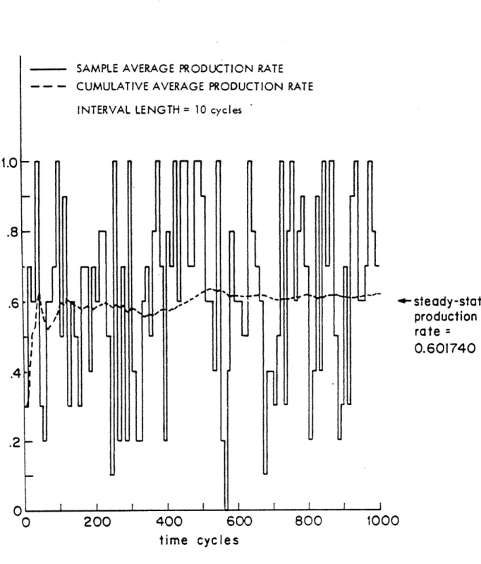
for a two-machine line and intervals of length 1. 126 Fig. 5.2 Sample and cumulative average production rates

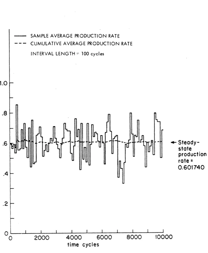
for a two-machine line and intervals of length 10. 127 Fig. 5.3 Sample and cumulative average production rates

for a two-machine line-and intervals of length 100. 128 Fig. 5.4 Sample and cumulative average production rates

for a two-machine line with small probabilities of

failure and repair. 130

Fig. 5.5 Sample and cumulative average production rates for a two-machine line with large probabilities of

failure and repair. 131

Fig. 5.6 Steady-state efficiency for two-machine transfer

lines. 140

Fig. 5.7 Steady-state line efficiency for a three-machine

transfer line with a very efficient third machine. 144

-7-Fig. 5.8 Steady-state line efficiency for a three-machine

transfer line with a very efficient first machine. 145 Fig. 5.9 Steady-state line efficiency for a three-machine

transfer line with identical machines. 146

Fig.5.10 Steady-state line efficiency for two-machine lines with the same first machine and different second

machines. 150

Fig.5.11 Steady-state line efficiency plotted against the efficiency in isolation of the second machine,

for two-machine lines with identical first machines. 151 Fig.5.12 The probability that the first machine in a

two-machine line is blocked, plotted against storage

capacity. 152

Fig.5.13 The probability that the second machine in a two-machine line is starved, plotted against storage

capacity. 153

Fig.5.14 Expected in-process inventory plotted against storage capacity, for two-machine lines with

identical first machines. 158

Fig.5.15 Expected in-process inventory as a fraction of storage capacity plotted against storage capacity, for two-machine lines with identical first

machines. 159

Fig.5.16 Expected in-process inventory as a fraction of storage capacity in the first storage plotted against the capacity of the second storage, for

a three-machine line. 164

Fig.5.17 Expected in-process inventory as a fraction of storage capacity in the second storage plotted against the capacity of the first storage, for

a three-machine line. 165

Fig. 6.1 Up-time frequency distribution for a two-machine

line with N=4. 176

Fig. 6.2 Up-time frequency distribution for a two-machine

line with N=8. 177

Fig. 6.3 Up-time frequency distribution for a two-machine

line with N=16. 178

Fig. 6.4 Down-time frequency distribution for a

two-machine line. 180

Fig. 6.5 Markov state transition diagram for a two-machine

transfer line with N=4. 183

-9-Fig. 6.7 Reduction of a three-machine line to an approximately equivalent two-machine line

by the aggregate method. 196

Fig. 6.8 Intuitive explanation of the 6-transformation. 199 Fig. 6.9 Efficiency against 6 for a two-machine line. 201 Fig.6.10 Obtaining the approximate efficiency of a

large system by solving a smaller system, by

the 6-transformation. 203

Fig. 7.1 Sketch of a roll products paper finishing

line. 210

Fig. 8.1 Schematic representation of a batch chemical

LIST OF TABLES

Tab. 2.1 Machine state transition probabilities. 46 Tab. 2.2 Storage level transition probabilities. 47 Tab. 3.1 Steady-state probabilities of two-machine line. 68 Tab. 3.2 Some boundary state probability expressions for

a three-machine transfer line. 71

Tab. 4.1 Two-machine line, lowest level, internal,

main-diagonal block. 87

Tab. 4.2 Two-machine line, lowest level, upper boundary

main-diagonal block. 89

Tab. 4.3 Three-machine line, lowest level, internal; main-diagonal block in second level upper

off-diagonal block. 90

Tab. 4.4 General form of the T' matrix. 97

Tab. 4.5 Theth level main-diagonal block. 105

Tab. 5.1 System parameters for dynamic simulation of

system transients. 125

Tab. 5.2 System parameters for dynamic simulation of

system transients. 129

Tab. 5.3 System parameters for two-machine lines. 139 Tab. 5.4 System parameters for three-machine lines. 143 Tab. 5.5 System parameters for two-machine lines. 149 Tab. 5.6 System parameters for a three-machine line. 163 Tab. 6.1 The number of system states in a k-machine

transfer line with buffer storage capacities

167 Tab. 6.2 System parameters for dynamic simulation. 170 Tab. 6.3 Estimates of parameters computed by taking

ratios of state frequencies from simulation

results. 171

Tab. 6.4 System parameters for output distributions of

a two-machine line. 175

Tab. 6.5 Steady-state probabilities of split states. 187 Tab. 6.6 Probability of producing exactly n pieces given

that the system has produced at least one piece,

for a two-machine line. 191

-10-Tab. 6.7 System parameters for 6-transformation. 200 Tab. 6.8 System parameters and line efficiencies for

various values of 6. 204

Tab. 6.9 System parameters and some boundary and

internal state probabilities for d-transformation. 206

Tab. 8.1 System parameters and line production rate for a

two-machine line with exponential service times. 235

Tab. 9.1 Steady-state probability distributions for

two-stage continuous lines. 246

Tab. 9.2 System parameters for continuous line. 254

Tab. 9.3 Efficiency for continuous and discrete lines for

1. INTRODUCTION

Complex manufacturing and assembly systems are of great importance, and their significance can only grow as automation further develops and enters more areas of production. At the same time, the balance between increased productivity and high cost is rendered more acute by the limitations on world resources, the precariousness of the economy, and the sheer volume of material involved. It is thus necessary to carefully study such systems, not only out of scientific inquisitiveness but also because of their important economical implications.

A suitable starting point in the study of production systems is the transfer line. For the purposes of the present work, a transfer line may be thought of as a series of work stations which serve, process, or operate

upon material which flows through these stations in a predetermined order.

Transfer lines are the simplest non-trivial manufacturing systems, and it appears that future work on more complex systems will by necessity be based on the concepts and methods, if not the results, derived in their study. Furthermore, transfer lines are already extremely widespread: they have become one of the most highly utilized ways of manufacturing or processing

large quantities of standardized items at low cost. Production line

principles are used in many areas, from the metal cutting industry, through the flow of jobs through components of a computer system, to batch

manufacturing in the pharmaceutical industry. At the same time, the accele-rated pace of life and crowded cities have institutionalized queues of people waiting to be served through series of stages, from cafeterias to vehicle inspection stations. The work presented here is devoted to methods of obtaining important measures of performance and design parameters for transfer lines, such as average production rate, in-process inventory, component reliability, and forced-down times.

The transfer line considered here may be termed unflexible: the material flowing through the system is of only one type, and must go though all the stations. A fixed sequence of operations is performed before the material is considered finished and can leave the system. Such a system can be studied

-12-

-13-as a special c-13-ase of flexible manufacturing systems.

The stations (also termed machines in the discussion that follows) are unreliable, in that they fail at random times and remain inoperable for random periods during which they are repaired. It is possible to-compensate for the losses in production caused by these failures by providing

redundancy, i.e. reserve machines that enter the network in case of failures. However, this is often prohibitively expensive, especially in the case of systems involving very costly components.

An alternative appears (Buzacott[1967a]) to have been discovered in the U.S.S.R. in the early fifties. This consists in placing buffer storages between unreliable machines in order to minimize the effects of machine failures. Buffers provide temporary storage space for the products of upstream machines when a downstream machine is under repair, and provide a temporary supply of unprocessed workpieces for downstream machines when an upstream machine is under repair. Although providing storage space and possibly machinery to move parts in and out of storages may be cheaper than redundancy of machines, the cost of floor space and in-process inventory are far from negligible. It is thus necessary to find in some predefined

sense the "best" set of storage capacities, in order to minimize cost while keeping productivity high. This leads to what may be refered to as

the buffer size optimization problem, which is discussed in section 1.1. Before this important optimization problem can be solved, however, the

effect of buffers on productivity, in-process inventory, and other measures of performance must be quantified. This quantification is the purpose of

-14-1.1 Considerations on the Economic Analysis of Interstage Buffer Storages

It is known from experimentation, simulation, and analysis that the average production rate and in-process inventory of a transfer line increase with buffer storage capacity. Before studying in detail the precise methods

for finding the relations between these parameters, however, it may be

necessary to describe the context for which they are intended. These results are considered in the optimal allocation of interstage buffer storage space. In some systems, it is desirable to maximize production rate; in others, such as lines that produce components to be assembled with parts produced elsewhere at known rates, it is desirable to keep the production rate as close as possible to a given value, while minimizing cost. In the former case, storages are often of significant value in increasing production rate and compensating for the losses due to the unreliability of machines. However, large storages mean high in-process inventory, a situation that is usually not desirable. In the latter case, ways will be described to find the least costly configuration of interstage buffers to give the desired production rate. In both cases, however, there is need for analysis techniques in

order to understand the exact relation between the various design parameters and performance measures.

Since production rate is known to increase with storage size,

maximizing production rate could be achieved by providing the system with very large buffers. However, there are important costs and constraints associated with providing buffers, including the costs of storage space and equipment, and in-process inventory. Thus, the buffer size optimization problem must take into account a number of constraints, including the following:

(i) There may be a limit on the total storage space to be provided to the line, i.e. on the sum of the capacities of all individual interstage buffer storages, due to cost of or limitations on floor space.

(ii) Furthermore, the capacity of each interstage storage may be limited due to limitations on floor space, or else, the weighted sum of storage

-15-capacities may be limited. This is the case, for example, if the system is an assembly line in which parts are mounted onto the workpieces so that their sizes increase in the downstream direction; this would not only necessitate tighter constraints on downstream storages, but it may also place a low upper limit on them because of floor space limitations.

(iii) It may be desirable to limit the expected (i.e. average) total number of jobs or parts in the system at any time, that is the in-process

inventory. (It may be noted that Elmaghraby[19661 calls only those parts that are actually being serviced in-process inventory, while he denotes those in the buffer storages as in-waiting inventory. Here, as in most other works, the term is taken to mean the material waiting in buffer

storages.) In-process inventory is an important consideration in.the

design and operation of manufacturing systems, particularly when the parts are costly or when delay is particularly undesirable due to demand for

finished products.

(iv) It may be necessary to limit the expected number of parts in certain storages only. This is the case, for example, if very costly elements are mounted onto the workpieces at a certain station, so that the in-process

inventory beyond that point must be limited; if parts equipped with the costly components are allowed to wait in storages, the time between the purchase or manufacture of the costly elements and the sale of the finished products may become long, and this is undesirable. More generally, since

each operation at subsequent stages gives more added value to each part, it may be necessary to weigh the cost of downstream inventory more than upstream inventory.

It may also be desirable to limit the amount of in-process inventory between certain specific stations. This is the case, for example, if a workpiece is separated into two parts at a certain station, and one of the parts is removed, possibly processed in a separate line or server, and the

two parts are then reassembled at some downstream station. In this case, it is not desirable to have large amounts of inventory waiting between the separation and assembly stations, since that would imply that at certain times, in the presence of failures, the ratio in which the two parts arrive

-16-at the assembly st-16-ation would significantly devi-16-ate from the desired one-to-one ratio. Complex network topologies, such as lines splitting and merging, separate lines sharing common servers or storage elements, are not treated here. The present work applies only to simple transfer lines. This is believed to be only a necessary first step towards the study of more complex systems.

It must be noted here that, as will be shown in section 5.3, items (i) and (ii) are not equivalent to (iii) and (iv). In other words, although limiting storage size certainly does impose an upper limit on the amount of in-process inventory, the relation between these two quantities is not necessarily linear.

The constraints outlined above are, of course, not exhaustive; specific applications may require additional considerations or constraints.

Calculating the costs involved in designing, building and operating transfer lines with interstage buffer storages involves numerous factors. Kay[1972] who studied the related problem of optimizing the capacity of conveyor belts by analytical as well as simulation techniques, found that conveyor capacity is an important parameter in the design of production systems. Yet, he found that none of the industrial designers that he encountered had considered this as a design parameter. The techniques and results presented here may serve the dual purpose of reiterating the

importance of methods and approaches for calculating the relation of buffer capacity and other design parameters to the performance of transfer lines.

The economic aspects of production lines with interstage buffer

storages have been studied by numerous researchers, in some cases by simu-lation, and in others by analytical methods based on queueing theory. Barten [19621 uses computer simulation to obtain mean delay times for material flowing through the system; he then bases his economic analysis on the cost of providing storage and labor and overhead costs as a function of delay time. Love[1967], who studied the related problem of modeling and policy optimization of a two-station (e.g. warehouse-retailer) inventory system, gives a cost model for inventory including the expected cost per time to operate the system, the cost of providing buffer facility, and that of the expected inventory at each storage. Soyster and Toof[1976] investigate the

-17-cost versus reliability tradeoff, and obtain conditions for providing a buffer in a series of unreliable machines. Young[1967] analyzes

multi-product multi-production lines and proposes cost functionals for buffer capacities, which he then uses in optimization studies by computer simulation. Kraemer

and Love[1970] consider costs incurred by in-process inventory as well as actual buffer capacity, and solve the optimal buffer capacity problem for a line consisting of two reliable servers with exponentially distributed service times and an interstage finite buffer storage.

The approaches proposed in these works may be followed in deriving appropriate cost models for an economic analysis of the system. It is beyond the scope of the present work to attempt to solve, or even formally

state, the buffer size optimization problem. For this reason, the economics of unreliable transfer lines with interstage buffer storages are not

discussed here in depth. It will suffice to list some of the important elements that must be considered in the cost analysis of such production systems. These include:

(i) Cost of increasing the reliability of machines. While the production rate generally increases with the reliability of individual machines, bottleneck stages eventually dominate. At the same time, increased machine

reliability involves increased capital cost, possibly due to additional research, high quality components, etc. In cases where machines are already chosen, there may be no control on their individual efficiency.

(ii) Cost of providing materials handling equipment for each storage. Buzacott[1967b] observes that providing storages involves a fixed cost, independently of the capacity of the storage, because of equipment needed to transfer pieces to and from the buffer, maintaining the orientation of the workpieces, etc. This complicates the decision problem on how many stages a production process must be broken into for optimal performance.

(iii) Cost of providing storage capacity. Floor space can be very expensive, so that buffer storages may involve considerable cost which is linear with the capacity of the buffer. It is sometimes possible, however, to use

alternate types of storage elements, such as vertical (chapter 7) or helical (Groover[19753) buffers, in order to reduce the area occupied by the buffer.

(iv) Cost of repair of failed machines. There is clearly a tradeoff between investing in increased machine reliability (item(i)) and in repairing

unreliable machines. Although this cost may not be controlled by providing interstage storages, it enters the design of transfer lines.

(v) Cost of maintaining in-process inventory. One of the major goals in production engineering is minimizing in-process inventory. This is

important not only when expensive raw material is involved, but also when the value added to the parts by machining is considerable.

(vi) Cost due to delay or processing time. Apart from the cost of operating the system, there may be a cost due to delaying the production or increasing the expected total processing time. This is especially true of transfer lines involving perishable materials, such as in the food, chemical, or pharmaceutical industries. Delay in response to demand is also an important consideration, although this is most important in flexible lines where the product mix may be changed to conform to demand.

(vii) The production rate of the system: the objective of the optimization problem is maximizing profit rate, a function of production rate as well as

cost rate. The latter involves labor and overhead costs, and may be computed in terms of mean-time needed to process a workpiece, including machining times, in-storage waiting times, and transportation. The former requires a more difficult analysis, since its relation to other system parameters such as reliability and storage size, is highly complex.

It is evident from this discussion that the problem of optimally designing a production line has many aspects. These include the choice of machines on the basis of reliability and cost; the division of the line into

stages once the machines have been chosen; and the optimal allocation of buffer capacity between these stages. Yet, the relations between these

steps and between the various design parameters are not well known, and most previous work in this area has centered on fully reliable lines, on simple

two-machine systems, or on simulation. The lack of analytical work on

unreliable lines with buffer storages has prompted Buxey, Slack and Wild[1973) to write "the only way to achieve realistic buffer optimization is through the use of computer simulations adapted to apply to specific rather than

-19-general situations." Numerical and analytical ways to obtain exact as well as approximate values for production rate, as well as some other performance measures, given the characteristics of the machines and storages,

-20-1.2 A Brief Review of Past Research

Transfer lines and transfer line-like queueing processes have been the subject of much research, and numerous approaches as well as results have been reported in the literature. The first analytical studies were the works of Vladzievskii[1952,1953] and Erpsher[1952], published in the U.S.S.R. in the early fifties.

Applications of queueing networks and transfer line models can be found in a large number of seemingly unrelated areas. These include the cotton industry (Goff[1970]), computer systems (Giammo[1976], Chandy[1972], Chandy, Herzog and Woo[1975a,1975b],Shedler[1971,1973], Gelenbe and Muntz

[1976], Baskett, Chandy, Muntz and Palacios[1975], Buzen[1971], Lam[1977], Konheim and Reiser[1976], Lavenberg, Traiger and Chang[1973], Wallace[1969], Wallace and Rosenberg[1966], etc.), coal mining(Koenigsberg[1958]), batch chemical processes (Stover[1956], Koenigsberg[1959]), aircraft engine

overhauling (Jackson[1956]), and the automotive and metal cutting industries (Koenigsberg[1959]).

A large portion of related research is based on the assumption that parts arrive at the first stage of the transfer line in a Poisson fashion. This greatly simplifies computation, and may be applicable to models of systems where parts arrive from the outside at a random rate, such as jobs in computer systems, people at service stations, cars at toll booths, etc. Most if not all of the computer-related work, as well as the results of Burke[1956], Hunt[1956], Avi-Itzhak and Naor[1963], Neuts[1968,1970], and Chu[1970] are based on the Poisson input assumption. As Soyster and Toof[1976) point out, however, this approach is not realistic when it comes to industrial systems such as assembly and production lines. Here, it is more reasonable to assume that parts are always available at the first stage, so that to follow Koenigsberg[1959], the approach may be termed "stochastic" as opposed to "queueing."

The production rate of transfer lines in the absence of buffers and in the presence of buffers of infinite capacity have been studied (Buzacott[1967a, 1968], Hunt[1956], Suzuki[1964], Rao[i975a], Avi-Itzhak and Yadin[1965],

-21-Morse[1965]). Some researchers have analyzed transfer lines with fully reliable components, in which the buffers are used to minimize the effects of fluctuations in the non-deterministic service times (Neuts[1968,1970], Purdue[1972], Muth[1973], Knott[1970a],Hillier and Boling[1966], Patterson

(1964], Hatcher[1969] (It should be noted that Knott[1970b] disputes

Hatcher's results and provides a counter-example)). Two-stage systems with finite interstage buffers have also been studied (Artamonov[1976], Gershwin

[1973a,1973b], Gershwin and Schick[19771, Gershwin and Berman[1978], Buzacott[1967a,1967b,1969,1972], Okamura and Yamashina[1977], Rao[1975a, 1975b], Sevast'yanov[1962]). Longer systems have been more problematic because of the machine interference when buffers are full or empty (Okamura and Yamashina[19773). Such systems have been formulated in many ways

(Gershwin and Schick[1977], Sheskin[1974,1976], Hildebrand[1968], Hatcher [1969], Knott[1970a,1970b]) and studied by approximation (Buzacott[1967a, 1967b], Sevast'yanov(1962], Masso and Smith[19741, Masso[1973]), as well as simulation (Anderson[1968], Anderson and Moodie[1969], Hanifin, Liberty and Taraman(1975], Barten[1962], Kay[1972], Freeman[1964]), but no analytic technique has been found to obtain the expected production rate of a multistage transfer line with unreliable components and finite interstage buffer storages.

-22-1.3 Outline of Research and Contributions

The present work aims at devising analytical, numerical, and

approximate methods for solving the problem of obtaining the production rate and other important performance measures of transfer lines with more than two unreliable stages and finite interstage buffers, while at the same time furthering the understanding of two-machine transfer lines.

The problem is formally stated in chapter 2: a description of the transfer line is followed by a state-space formulation in section 2.1, and a discussion of the modeling assumptions in section 2.2. The Markov chain model is introduced and discussed in section 2.3.

An analytical approach is developed in chapter 3: the states of the system are classified as internal and boundary, and these are studied in sections 3.1 and 3.2 respectively. A sum-of-products solution for the steady-state probabilities of internal states of the system is introduced in section 3.1.2, and the analysis is extended to the boundary states for two-machine lines, and three-machine and longer lines, in sections 3.2.1 and 3.2.2 respectively.

Numerical methods for solving the transfer line problem are developed in chapter 4: the iterative multiplication scheme known as the power method is introduced and discussed in section 4.1. An algorithm which solves the large system of transition equations by taking advantage of the sparsity and block-tri-diagonal structure of the transition matrix is developed in section 4.2: the structure of the transition matrix is studied in section 4.2.1 and the algorithm is formulated in section 4.2.2. Some important

computer storage problems associated with this algorithm are discussed in section 4.2.3.

The state probabilities obtained by the analytical and numerical

methods discussed in chapters 3 and 4 are used to calculate important system performance measures in chapter 5: these include efficiency and production rate, forced-down times, and in-process inventory. The production rate of the system is discussed in section 5.1: alternate ways to compute production rate are given in section 5.1.1, and the effects of start-up transients on

-23-this quantity are investigated by dynamic simulation in section 5.1.2.

The dependence of production rate, forced-down times and expected in-process inventory on the failure and repair rates of individual machines and the capacities of individual storages is studied in sections 5.1.3, 5.2, and 5.3 respectively.

Approximate methods for computing the system's production rate with less computation than is required by the exact methods developed in earlier chapters are introduced in chapter 6: dynamic simulation and its limited uses in the present work are briefly reviewed in section 6.1. An aggregate method for computing the approximate average production rate of a long transfer line is introduced in section 6.2: this method is based on the quasi-g.eometric input and output characteristics of two-machine lines, as demonstrated in section 6.2.1. Since a single machine has exactly geometric input and output characteristics, the approximate equivalence of a single machine to a two-machine, one-storage segment of a transfer line is

proposed in section 6.2.2. It is shown, however, that the approximation is best when the line is not well balanced, a rare occurrence in actual

industrial systems. A mathematical operation on the system parameters. referred to as the 6-transformation is introduced in section 6.3.1. It is

shown in section 6.3.2 that this transformation leaves production rate nearly unchanged. The major consequence is that the state space can be considerably reduced through this approach, thus decreasing the amount of computation and memory necessary to solve the problem.

Chapters 7,8, and 9 are devoted to applications of the theory. The aim of these chapters is primarily to demonstrate the wide-range applicability of the model, while at the same time pointing out its shortcomings and

weaknesses and discussing ways of extending the model to more closely conform to actual situations.

Chapter 7 outlines a paper finishing line: this system is shown to lend itself to a three-machine, two-storage transfer line model, although several important differences exist between the system and the model. These are discussed in section 7.1, while attempts at modeling the system are reviewed in section 7.2.

-24-Chapters 8 and 9 investigate the application of the transfer line model to chemical systems. It appears that Stover's [1956] pioneering work in the application of queueing theory to chemical plants has not been

followed up or developed subsequently. Yet, as is shown here, this approach can be particularly useful in estimating the production rates of chemical systems in the presence of unreliable equipment: pumps or valves that fail, heating, cooling, or control mechanisms that break down, etc.

A queueing theory approach to the study of batch chemical processes, in which pumps, reactors, and other unreliable components are represented by machines and holding tanks by storages, is introduced in section 8.1. Major differences between actual systems and the model are discussed in sections 8.1.1 and 8.1.2. The model is extended to account for cases where servicing times are not deterministic. This includes reactors where batches of chemicals take periods of time which deviate from a known mean holding time to reach a desired conversion. This may happen because of variations in the temperature or concentration of the feed, or because the kinetics of the reaction are not understood well enough to predict reaction times exactly. The new model is applied to a simple system consisting of a batch reactor and a still, separated by unreliable pumps and parallel holding tanks, in section 8.2.1. A numerical example is worked out, and more complex systems are discussed, in sections 8.2.2 and 8.2.3 respectively.

The 6-transformation introduced in section 6.3 is taken to its limit as 6+0 and the model is shown to become equivalent to a continuous system in chapter 9. Results obtained by differential equations for a continuous

line are outlined in section 9.1, and the limiting case of the 6-transformation is studied in section 9.2. The two approaches are shown to yield identical results. A numerical example of a continuous chemical process, in which a plug-flow reactor and a distillation column are separated by unreliable pumps and a holding tank is worked out.

2. PROBLEM STATEMENT AND MODEL FORMULATION

Formulating a mathematical model in order to study the relations between certain parameters and measures of performance in transfer lines requires a formal and unambiguous statement of the problem.

Section 2.1 gives a general description of a multistage transfer line with unreliable components and interstage buffer storages. The line is

discussed in section 2.1.1 and a state space formulation is introduced in section 2.1.2.

The various assumptions made in the process of translating the system into a mathematical model are outlined and discussed in section 2.2. These assumptions are necessary in order to render the mathematical model

tractable, while not losing sight of the physical properties of the actual system. Many of these assumptions are standard (Feller[1966], Koenigsberg

[1959]). The assumptions are stated, justification is given, and possibilities of relaxation are investigated.

The Markov chain approach to modeling the transfer line is discussed in section 2.3. This approach is frequently used in the study of queueing networks arising from computer systems (Wallace[1972,1973], Wallace and Rosenberg[1966]) or manufacturing systems (Buzacott[1967a,1967b,1969,1971, 1972]). A brief review of the properties of Markov chains is given in

section 2.3.1. (An excellent and exhaustive text on Markov systems is Howard [19711). The Markov model of the transfer line is discussed in section 2.3.2.

-25-

-26-2.1 Modeling the Transfer Line

2.1.1 Description of a Multistage Transfer Line with Buffer Storages

The system under study is illustrated in figure 2.1. It consists of a linear network of machines separated by buffer storages of finite capacities. Workpieces enter the first machine from outside the system. Each piece is processed (drilling or welding in a metal cutting line, reacting or

distillating in a chemical plant, data processing in a computer network, etc.)

by machine 1, after which it is moved into storage 1. For the purposes of this study, the nature of the machine operation may be ignored, and a machine is taken to be an unreliable mechanism which moves one workpiece per cycle in the downstream direction. The buffer is a storage element in which a workpiece

is available to a downstream machine with a negligible delay. The part moves in the downstream direction, from machine i to storage i to machine i+l and so on, until it is processed by the last machine and thereby leaves the system.

Machines fail at random times. While some of these failures are easy to diagnose and quick to repair, such as some tool failures, temporary power

shortages, etc., others involve more serious and time-consuming breakdowns, such as jamming of workpieces or material shortages. Thus, the down-times of the machines, like the up-times, are random variables. When a failure occurs, the level in the adjacent upstream storage tends to rise due to the arrival of parts produced by the upstream portion of the line; at the same time, the level

in the downstream adjacent storage tends to fall, as the parts contained in that storage are drained by the downstream portion of the line. If the failure lasts long enough, the upstream storage fills up, at which time the machine immediately preceeding it gets blocked and stops. Similarly, given that the failure takes long enough to repair, the downstream storage eventually empties,

and causes the machine following it to starve and stop. This effect propagates

up and down the line if the repair is not made promptly.

If it is assumed that machines cannot operate faster than their usual rates in order to catch up the time lost because of such failures, it is clear that

-27- r-0 I _ _t a) i o r~~~~~~~~r .4--0~~~~~~~~~~-* 00_.c -, _,O 0-

II

-28-breakdowns have the effect of reducing the average production rate of the transfer line. Although machine failures are to a certain extent inevitable, it is desirable to avoid situations in which operational machines are

affected by failures elsewhere and are forced to stop. Such situations can to a certain extent be avoided by the use of buffer storages, which act so as to partially decouple adjacent machines. As the capacities of these storages are increased, the effects of individual failures on the production rate of the system are decreased.

It is desirable to study the interactions between the elements of the system and the relations between various system parameters, so as to be able to quantify the advantages of using buffer storages and their

-29-2.1.2 State Space Formulation

A probabilistic approach is taken in the study of unreliable transfer lines. Starting with probabilities of failure and repair for each individual machine in the line, the probabilities of producing a piece, of being forced down, or of having a given number of parts in a given storage within any time cycle are sought. These are used in evaluating the system's performance. The transfer line problem was studied through such a probabilistic approach for the first time (see Buzacott[1967a]) by Vladzievskii[1952].

In order to carry out the analysis in this direction, it is necessary to formulate a state space for the probabilistic model. A system state is defined as a set of numbers that indicate the operational status of the machines and the number of pieces in each storage, as described below.

For each machine in a k-machine line, the variable a. is defined as follows:

0 if machine i is under repair

6.=aid~~~~~ |i=l,..,k (2.1)

i

1 if machine i is operational

It is important to note that operational is defined to mean "capable of processing a piece," as opposed to "actually processing a piece." This accounts for cases where the machines are in good working order, but are not processing parts because they are starved or blocked. Several authors

(Haydon[1972], Okamura and Yamashina[1977], Kraemer and Love[1970]) define four states, by adding to the above separate states for blocked and starved machines. It will be shown, however, that since probabilities of transition between states are taken here to depend not only on the states of machines but also on the levels of storages, the two approaches are equivalent, though the one given by equation (2.1) is more compact.

The variable n. is defined as the number of pieces in (the level of) storage j. Each storage is defined to have a finite maximum capacity N , so that

-30-o

J ]

The state of the system at time t is defined to be the set of numbers

s(t) = (n_{l ( t)} r,. .,n k-l (t ), (t )l . . k( (2.3)

It may be noted that time, though denoted by the letter t, is discrete. As will be described in section 2.2.2, time is measured in machining cycles.

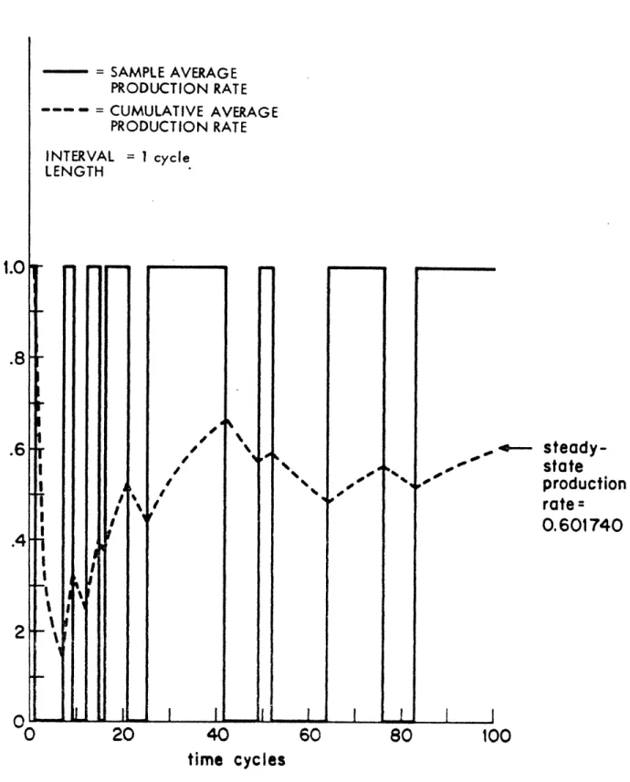
The efficiency of a transfer line is defined to be the probability of producing a finished piece within any given cycle. It may be thought of as the expected ratio of time in which the system actually produces finished parts to total time. Efficiency, E, satisfies

0 < E < 1 (2.4)

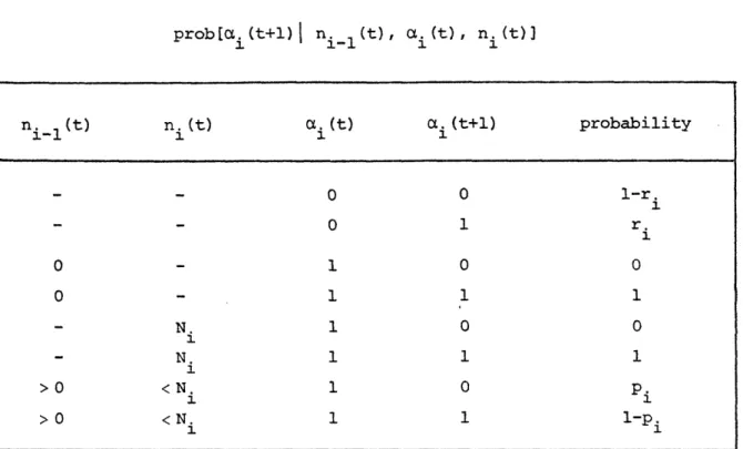
State transition probabilities are treated in section 2.2.3. Methods of obtaining steady state probabilities are developed in chapters 3 and 4, and their relation to efficiency are discussed in chapters 5 and 6.

-31-/2.2 Assumptions of the Model

/

2.2.1 Input and Output of the Transfer Line

It is assumed that an endless supply of workpieces is available upstream of the first machine in the line and an unlimited storage area downstream of the last machine is capable of absorbing the parts produced by the line. Thus, the first machine is never starved and the last machine is never blocked.

Although a large portion of computer-related work assumes that jobs arrive at the system at random rates, often in Poisson fashion, it is more realistic in industrial systems to assume that parts are available when needed (Soyster and Toof[1976]). Nevertheless, it is possible to think of

cases in which delays in reordering raw materials etc. may cause a shortage of workpieces at the head of the line. Similarly, it is conceivable that

congestion downstream in the job shop may cause blocking at the end of the line. These events would clearly not have Poisson time distributions: in that case, parts arrive singly, with random interarrival times. In most industrial cases, it may be expected that parts are delivered in batches. In such cases, it is possible to think of the first and last machines in the model as representing loading and unloading stations. Then, temporary shortages of workpieces or temporary congestion downstream may be modeled as failures in these machines. In other words, unreliable first and last machines may model delivery to and from the production line, especially if parts are moved in bulks (Bagchi and Templeton[l972]).

A single machine, i.e. a one-machine line, stays up for a random length of time, and once a failure occurs, it remains down for a random length of time. Both of these periods are geometrically distributed (as will be shown in section 2.2.3). Thus, the arrival of bulks (or batches) of geometrically distributed sizes, with geometrically distributed interarrival times, may be modeled by a fictitious first machine. This may involve some additional considerations, however. Subsequent deliveries must be independent, and the first storage may have to have infinite capacity.

-32-In general, the assumption of infinite workpiece supply will be

justified for most industrial applications. Entire production lines seldom have to stop because of lack of raw material; major shutdowns due to strikes or accidents are of an entirely different nature and are not considered

stochastic failures in the sense described in section 2.2.3. There may, nevertheless, be cases where loading and unloading batches takes some time. This is the case, for example, with the paper finishing line (chapter 7) where paper is supplied to the line in the form of extremely large, but necessarily finite rolls. As discussed in section 7.1.2, the effect of starving the line during loading may be ignored if the period of time in which the system is starved is negligible compared to other times involved in the system.

-33-2.2.2 Service Times of the Machines

It is assumed that all machines operate with equal and deterministic service times. The temporal parameter t is chosen so that one time unit is equal to the duration of one machine cycle. Thus, the line has a production rate determined only by its efficiency. The efficiencies of individual machines in isolation, on the other hand, are functions of their mean times between failures and mean times to repair, or alternately their repair and

failure probabilities. (This is discussed in detail in section 5.1). Although deterministic service times may be encountered in certain actual systems (Koenigsberg[1959] mentions an automobile assembly line), this assumption does not hold in many industrial applications. Not only is machining time often a random variable, but downstream machines frequently

operate on the average at a faster rate than upstream ones, in order to avoid as much as possible the blocking of upstream machines.

The assumption of constant machining times is justifiable if service times do not deviate appreciably from the mean, compared to the mean service time. This is because variances in service times do not significantly affect the system behavior and average production rate at the condition that the system is not driven to boundaries, i.e. storages are not emptied or filled up. As will be shown in later chapters, the largest steady-state probabilities belong to states with 1 or Ni-l pieces in storages. Thus, the system runs most often near boundaries. As a result of that, small deviations from the mean may average out, although large deviations may starve certain machines and block others, thereby reducing the line production rate.

Solutions have been obtained for queueing networks with servers having exponential time distributions (See section 8.2). The assumption of exponential distribution reduces the complexity of the problem, but numerous researchers point out that this is often not a reasonable assumption (e.g. Rao[1975a]). Gaussian distributions have been proposed by some (Vladzievskii[1952],

Koenigsberg[1959]) and certain Erlang (See Brockmeyer, Halstrrm and Jensen[1960])

distributions may be considered in that they have applicability to industrial

cases and satisfy the Markov proper-y o= no memory (Section 2.3). Transportation takes negligible time compared to machining times.

-34-2.2.3 Failure and Repair of Machines

Machines are assumed to have geometrically distributed times between failures and times to repair. This implies that at every time cycle, there is a constant probability of failure given that the machine is processing a piece, equal to the reciprocal of the mean time between failures (MTBF).

It is further assumed that machines only fail while processing a piece. Similarly, there is a constant probability of repair given that the machine has failed, equal to the reciprocal of the mean time to repair (MTTR).

The assumption of geometric failure rate is common (Vladzievskii[1952], Koenigsberg[1959], Esary, Marshall and Proschan[1969], Barlow and Proschan

[1975], Goff[1970], Buzacott[1967a,1967b,1969], Feller[19661, Sarma and Alam [1975]). It makes it possible to model the system as a Markov chain, since it satisfies the memoryless property of Markov systems (Section 2.3). However, there are certain difficulties with this assumption. While it

applies to those cases where the overwhelming majority of failures are due to accidental, truly stochastic events, such as tool breakage or workpiece

jams, it does not account for scheduled down-times or tool wear. Such stoppages are predictable given knowledge of the history of the system. Yet, when there is a very large number of possible causes of failure, so that even if some are scheduled, the time distribution including stochastic failures is close to a geometric distribution, this assumption can be made.

Geometric repair time distributions imply that the repair is completed during any cycle with a constant probability, regardless of how long repairmen have been working on the machine. This assumption may not be far from the truth if there are many possible causes of failure, each of which take different

lengths of time to repair.

Some examples of actual up- and down-time distributions from an industrial manufacturer appear in figures 2.2 and 2.3. Although these are for relatively

small numbers of runs, totalling no more than several hundred time cycles, the distribution is in fact seen to be remarkably close to geometric. (These charts

represent typical data obtained from an industrial manufacturer. The actual data is the proprietory information of the industrial manufacturer.)

-35-CM t0 C o.C₁ cqj 0 04-( a -,-. En .-ic .- _ H -H a, r:

\,,,GuoL

,

f,1,,qq,

,

E,,

-36-Q. a) p / EDo Qr) a)

abuoqo ajojS

lo

Af!I!qoqOJd

0j

X_ V) C) U)

0 -H

abtuo40 ajoc

S

o ~l!!qoqoid

"

-37-The model does not take into account the problem of machine interference (Benson and Cox[1951], Cox and Smith[1974]), in which the limited number of repairmen affects the repair probabilities when more than one machine are down simultaneously. Not only are the repair probabilities reduced in such cases, but they further depend on which machine broke down first, since the repairmen will be at work at that machine with greatest probability. Ways of taking this problem into account are discussed to some detail in section 7.1.6.

While repair takes place independently of storage levels or the number of failed machines, a failure can only occur when the machine is actually processing a part. This implies that the upstream storage is not empty and the downstream storage is not full. In the former case, the machine has no workpiece to operate on, and in the latter, it is not allowed to operate since

there is no place to discharge a processed workpiece. In other words, a forced-down machine cannot fail. In research reported by Koenigsberg[1959], Finch assumed that forced-down machines have the same probability of failure

as running machines, an assumption that is not realistic.(Buzacott[1967a,1967b], Okamura and Yamashina[1977]).

The assumption that machines only fail while actually processing a piece is consistent with the assumption that the great majority of failures is due to stochastic events such as tool breakage, as opposed to scheduled shutdowns or major system failures that may happen at any time.

-38-2.2.4 Conservation of Workpieces

The model does not account for any mechanism for destroying or rejecting workpieces, or for adding semi-finished workpieces into the line. Thus, the

average rate at which pieces are processed by each stage in the line is the same for all stages. It is shown in section 5.1.1 that the solution to the two-machine line satisfies the conservation of pieces. The proof is not complete for longer lines.

The fact that pieces are not created by the system is true except when machines cut workpieces into identical parts, all of which are then processed by downstream machines; this is the case in the paper finishing line (See

section 7.1.1). That pieces are not destroyed, however, assumes that a workpiece is not scrapped when a machine fails while processing it (as in

the work of Okamura and Yamashina[19773), that there are no interstage inspection stations where defective parts are removed, etc. In systems

satisfying these requirements, all stages process the same average number of pieces per cycle, and it is thus only necessary to compute the production

rate of one stage, e.g. the last one (Koenigsberg[1959]). There is an

importantexception to this rule, and that involves infinite buffer storages for which the upstream portion of the line is more efficient than the

downstream portion. This is examined in greater detail in section 5.1.3. Cases in which workpieces are cut into parts or parts are assembled or packaged together are briefly treated in section 7.1.1. It is possible to approximate such lines by considering the smallest part as a unit and analyzing larger parts, either before they are cut or after they are

assembled, as multiples of the smallest unit. This approach is not exact, and errors are introduced by effective changes in the flexibility of the system.

-39-2.2.5 Dynamic Behavior of the System

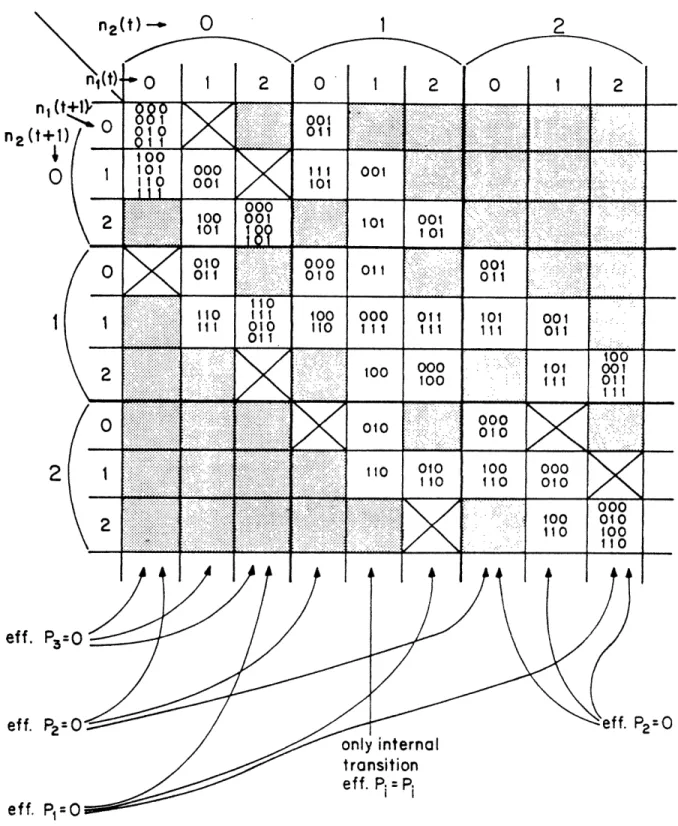
It is assumed as a convention that machines make their state transitions first, conditional on the level of the adjacent storages. Once these changes take place, the storage levels undergo state transitions, within the same time cycle. This is only a convention and the actual system does not have to

operate this way. Thus, the transition a. i(t)-*ai(t+l) is conditional on i(t),. ni ₁ (t) and ni(t). However, the transition n (t)-+n (t+l) is conditional on ni _l(t),ni(t),ni+l(t), as well as ai(t+l) and ai+l(t+l), where these latter indices are the final machine states while the former are the initial storage states. Note that the machine and storage transitions depend only on the adjacent machine and storage states, and do not depend on the states of machines and storages further removed.

This assumption makes the computation easier, because it implies that the final storage state is uniquely determined once the initial storage states and the final machine states are known. The advantages of this approach in the mathematical derivation are made clearer in section 3.1.1.

This assumption is consistent with those stated previously: a machine

can not fail if the adjacent upstream storage is empty, so that there are no parts to process, or if the adjacent downstream storage is full, so that there is

no place to put the processed piece. Furthermore, a piece is not destroyed when a machine fails, but merely remains in the upstream storage until the machine is repaired. Finally, since all machines work synchronously, there

is no feed forward information flow, so that the knowledge that a place will be vacant in the downstrean storage or that a piece will emerge from the

upstream machine in the time cycle to follow does not influence the decision on whether or not to attempt to process a piece.

It is important to note that this is mostly for mathematical convenience and need not represent the operation of the actual system. One consequence of this assumption is important, however, and must be consistent with the actual system. Because there is no feed forward information flow, a machine can not decide to process a piece if the upstream storage is empty, even though the upstream machine may be ready to discharge a part. Similarly, the machine

-40-cannot start processing a piece if the downstream storage is full, even though the downstream machine may have just been repaired and is ready to take in a piece. Thus, there is a delay of at least one cycle between

subsequent operations by adjacent machines on any given workpiece, and between a change in the system state and decisions on the part of the machines towards the next state transition. This is unlike the models analyzed by Hatcher[1969] and Masso[1973], in which a part may emerge from a machine and go into the next, bypassing the storage element, within the same time cycle.

-41-2.2.6 The Steady State Assumption

It is assumed that the probabilistic model of the system is in steady state, i.e. that all effects of start-up transients have vanished and that the system may be represented by a stationary probabilistic distribution.

A stochastic system is never at rest. Thus, as explained in section 5.1.2, the steady state assumption does not imply that the system is not fluctuating. What it does imply is that a sufficiently long period of time has passed since start-up, so that knowledge of the initial condition of the system does not give any information on the present state of the system. Thus, the average performance of the system approaches the steady state values calculated by assuming that the probabilistic model of the system is stationary.

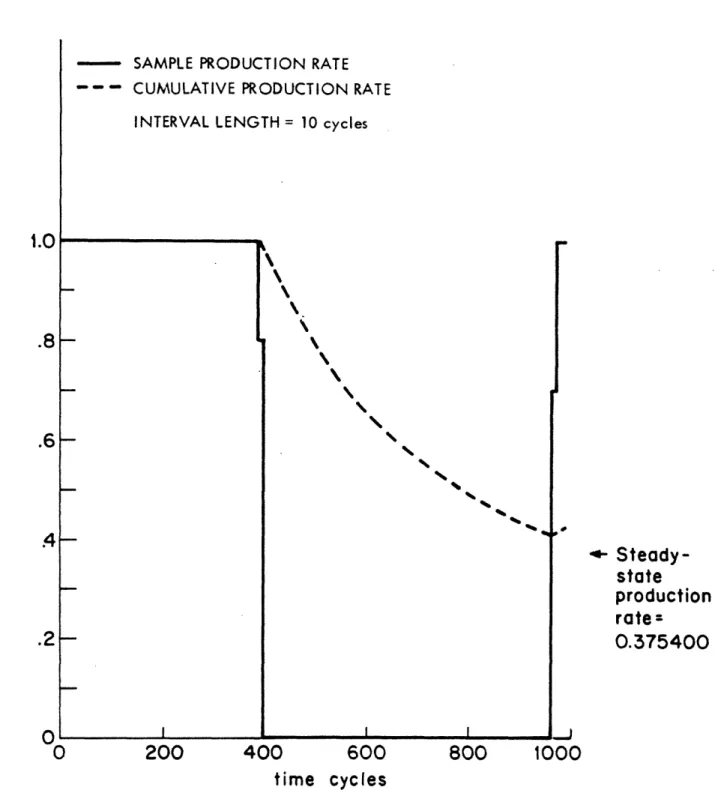
There may be cases, however, in which transients take very long to die down, compared to the total running time of the system. In such cases, the steady state values may not represent the average performance of the system. The effects of start-up transients are briefly discussed in section 5.1.2.

-42-2.3 Formulation of the Markov Chain Model

2.3.1 The Markovian Assumption and Some Basic Properties

A stochastic process may be defined as a sequence of events with random outcomes. A process is said to be Markovian if the conditional joint probability distribution of any set of outcomes of the process, given some state, is

independent of all outcomes prior to that state. Thus, defining the state of the system at time t as s(t),

p[s(t+l) s(t),s(t-1),, s(t-))] = p[s(t+l) s(t)] (2.5)

This implies that at any given time, the transition probability depends only on the state occupied at that time; it is independent of the past history of transitions. Another way of saying this is that the transition from one

state to another is independent of how the system originally got to the first state. This is what is meant by the memorylessness of Markov processes.

The expression appearing on the right-hand-side of equation (2.5) is the probability of transition from the state occupied at a given time to the state occupied one time step later. This probability is assumed to be

independent of time. Thus, the state transition probabilities are defined as

t.. = p[s(t+l)=jIs(t)=i] ; all i,j (2.6)

Given that there are M states, the transition probabilities defined by equation (2.6) obey the following relations:

t..j 0 ; all i,j (2.7)

t.. = 1 ; all i (2.8)

j=1 ti

-43-The transition matrix is defined as

tll t21 ... tM1 t12 t22

T = . . (2.9)

t

At time t, the probabilities that the system is in state i=l,..,M may be represented as a state probability vector, defined as

p1(t) p[s(t)=l] P₂(t) p(s(t)=2] P2 (t) P(t) = . . (2.10) PM(t) p[s(t)=M] where M EPi (t) = 1 (2.11) i=l

Then, the state probability vector at time t+l is given by

p(t+l) = T p(t) (2.12)

and recursive application of equation (2.12) gives

(t) = T p(O)

A

(t)

P(0)

(2.13)

Here, p(0) is a given initial (a priori) probability vector, and Tt denotes th

-44-limit

lim (t) A (2.14)

tom

exists and if the steady-state probability vector defined as

Ap p(0) = (2.15)

is independent of the value of the initial state probability vector p(0). As t4-, equation 2.12 becomes

p = T p (2.16)

since the vectors p(t) and p(t+l) converge to p.

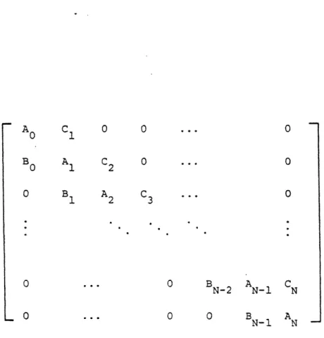
Equations (2.11) and (2.16) are shown to uniquely determine the value of p for the system under study in section 4.2.1. These two equations form the basis of both analytical methods derived in chapter 3 and the sparse block tri-diagonal system of equations solving algorithm introduced in section 4.2. The power method discussed in section 4.1 is based on equations