HAL Id: hal-00341609
https://hal.archives-ouvertes.fr/hal-00341609
Submitted on 25 Nov 2008
HAL is a multi-disciplinary open access
archive for the deposit and dissemination of
sci-entific research documents, whether they are
pub-lished or not. The documents may come from
teaching and research institutions in France or
abroad, or from public or private research centers.
L’archive ouverte pluridisciplinaire HAL, est
destinée au dépôt et à la diffusion de documents
scientifiques de niveau recherche, publiés ou non,
émanant des établissements d’enseignement et de
recherche français ou étrangers, des laboratoires
publics ou privés.
Reuven Cohen, Pierre Fraigniaud, David Ilcinkas, Amos Korman, David Peleg
To cite this version:
Reuven Cohen, Pierre Fraigniaud, David Ilcinkas, Amos Korman, David Peleg. Label-Guided Graph
Exploration by a Finite Automaton. ACM Transactions on Algorithms, Association for Computing
Machinery, 2008, 4 (4), pp.Article 42. �10.1145/1383369.1383373�. �hal-00341609�
by a Finite Automaton
REUVEN COHENBoston University, USA PIERRE FRAIGNIAUD
CNRS and Universit´e Paris Diderot - Paris 7, France DAVID ILCINKAS
CNRS and Universit´e Bordeaux I, France. AMOS KORMAN
CNRS and Universit´e Paris Diderot - Paris 7, France and
DAVID PELEG
The Weizmann Institute, Rehovot, Israel.
A finite automaton, simply referred to as a robot, has to explore a graph, i.e., visit all the nodes of the graph. The robot has no a priori knowledge of the topology of the graph or of its size. It is known that, for any k-state robot, there exists a graph of maximum degree 3 that the robot cannot explore. This paper considers the effects of allowing the system designer to add short labels to the graph nodes in a preprocessing stage, and using these labels to guide the exploration by the robot. We describe an exploration algorithm that given appropriate 2-bit labels (in fact, only 3-valued labels) allows a robot to explore all graphs. Furthermore, we describe a suitable labeling algorithm for generating the required labels, in linear time. We also show how to modify our labeling scheme so that a robot can explore all graphs of bounded degree, given appropriate 1-bit labels. In other words, although there is no robot able to explore all graphs of maximum degree 3, there is a robot R, and a way to color in black or white the nodes of any bounded-degree graph G, so that R can explore the colored graph G. Finally, we give impossibility results regarding graph exploration by a robot with no internal memory (i.e., a single state automaton).
Categories and Subject Descriptors: C.2.1 [Computer-communication networks]: Network Architecture and Design; C.2.2 [Computer-communication networks]: Network Protocols; C.2.4 [Computer-communication networks]: Distributed Systems; E.1 [Data Structures]:
Author’s address: Reuven Cohen: Dept. of Electrical and Computer Eng., Boston University, Boston, MA, USA. E-mail: [email protected]. Supported by the Pacific Theaters Foundation. Pierre Fraigniaud: CNRS and Universit´e Paris Diderot - Paris 7, France. E-mail: [email protected]. Supported by the project “PairAPair” of the ACI Masses de Donn´ees, the project “Fragile” of the ACI S´ecurit´e et Informatique, and by the project “Grand Large” of INRIA.
David Ilcinkas: CNRS and Universit´e Bordeaux I, France. E-mail: [email protected]. Amos Korman: CNRS and Universit´e Paris Diderot - Paris 7, France. E-mail: [email protected]. Supported in part by the project “GANG” of INRIA.
David Peleg: Dept. of Computer Science, The Weizmann Institute, Rehovot, Israel. E-mail: [email protected]. Supported in part by a grant from the Israel Science Foundation. Permission to make digital/hard copy of all or part of this material without fee for personal or classroom use provided that the copies are not made or distributed for profit or commercial advantage, the ACM copyright/server notice, the title of the publication, and its date appear, and notice is given that copying is by permission of the ACM, Inc. To copy otherwise, to republish, to post on servers, or to redistribute to lists requires prior specific permission and/or a fee.
c
Distributed data structures, Graphs and networks; G.2.1 [Discrete mathematics]: Combina-torics; G.2.2 [Discrete mathematics]: Graph theory
General Terms: Algorithms, Theory
Additional Key Words and Phrases: Distributed algorithms, Graph exploration, Labeling schemes
1. INTRODUCTION 1.1 Background:
This paper concerns graph exploration by finite automata. Let R be a finite au-tomaton, simply referred to in this context as a robot, moving in an unknown undirected graph G = (V, E). The robot has no a priori information about the topology of G and its size. To allow the robot R to distinguish between the dif-ferent edges of a node u while visiting it, the d = deg(u) edges incident to u are associated with d distinct port numbers in {0, . . . , d − 1}, in a one-to-one manner. The port numbering is given as part of the input graph, and the robot has no a priori information about it. For convenience of terminology, we henceforth refer to the edge incident to port number l at node u simply as “edge l of u”. (Clearly, if this edge connects u to v, then it may also be referred to as “edge l′ of v” for the
appropriate l′.) The robot has a finite number of states and a transition function
f . If R enters a node of degree d through port i in state s, then it switches to state s′ and exits the node through port i′, where (s′, i′) = f (s, i, d). The objective of
the robot is to explore the graph, i.e., to visit all its nodes. The size of the robot’s memory equals the logarithm of the number of states.
The first known algorithm designed for graph exploration was introduced by Shannon [Shannon, 1951]. Since then, several papers have been dedicated to the feasibility of graph exploration by a finite automaton. Rabin [Rabin 1967] conjec-tured that no finite automaton with a finite number of indistinguishable pebbles can explore all graphs (a pebble is a marker that can be dropped at and removed from nodes). The first step towards a formal proof of Rabin’s conjecture is gen-erally attributed to Budach [Budach, 1978], for a robot without pebbles. Blum and Kozen [Blum and Kozen, 1978] improved Budach’s result by proving that a robot with three pebbles cannot perform exploration of all graphs. Kozen [Kozen, 1979] proved that a robot with four pebbles cannot explore all graphs. Finally, Rol-lik [RolRol-lik 1980] gave a complete proof of Rabin’s conjecture, showing that no robot with a finite number of pebbles can explore all graphs. The result holds even when restricted to planar 3-regular graphs. Without pebbles, it was proved [Fraigniaud et al., 2005] that a robot needs Θ(D log ∆) bits of memory for exploring all graphs of diameter D and maximum degree ∆. On the other hand, if the class of input graphs is restricted to trees, then exploration is possible even by a robot with no memory (i.e., zero states), simply by depth-first search (DFS) using the transition function f (i, d) = i + 1 mod d (see, e.g., [Diks et al., 2004]).
Two variants of the exploration problem have been addressed in the literature: ex-ploration with stop (in which the robot has to complete exex-ploration and eventually stop) and exploration with return (in which the robot has to perform exploration and return to its starting position). It is shown in [Diks et al., 2004] that exploration
with stop of n-node trees requires a robot with memory size Ω(log log log n) bits, and in [Gasieniec et al., 2007] that exploration with return of n-node trees can be achieved by a robot with O(log n) memory bits. It is impossible to explore arbitrary graphs with stop by a single robot if no marking of nodes is allowed. In [Fraigniaud et al., 2005], the authors show that also using one pebble, the exploration with stop of n-node graphs requires a robot with memory size Ω(log n) bits.
1.2 Label-guided exploration:
The ability of dropping and removing pebbles at nodes can be viewed alternatively as the ability of the robot to dynamically label the nodes. If the robot is given k pebbles, then at any time during the exploration,Pu∈V |lu| ≤ k, where lu is the
label of node u and |lu| denotes the size of the label in unary.
In certain settings, it is expected that the graph will be visited by many ex-ploring robots, and consequently, it is desired to preprocess the graph by leaving fixed (preferably small) road-signs, or labels, that will aid the robots in their ex-ploration task. As a possible scenario, one may consider a network system where finite automata are used for traversing the system and distributing information in a sequential manner. Recently, a number of papers studied the affects of assigning (short) labels in a preprocessing stage, in order to ease a distributed task (e.g., [Korman et al., 2005; Fraigniaud et al., 2006; Fraigniaud et al., 2007]). This paper considers the affects of allowing the system designer to assign labels to the nodes in a preprocessing stage, and using these labels to guide robot explorations. The transition function f is augmented to utilize labels as follows. If the robot R in state s enters a node of degree d, labeled by l, through port i, then it switches to state s′ and exits the node through port i′, where
(s′, i′) = f (s, i, d, l).
This model can be considered stronger than Rabin’s pebble model since labels are given in a preprocessing stage, but it can also be considered weaker since, once assigned to nodes, the labels cannot be modified.
Remark. It should be noted that the general function f presented here may depend on d, i and l, all of which may require log n bits to be described in an n-node graph. However, our formalism fits in the standard context of Mealy automata, i.e., the number of states of the robot is independent from the sizes of the inputs and outputs of the transition function. In contrast, for Moore automata, the output of the transition function is a state, in which the output port number is encoded, and thus the number of states of a Moore automaton is at least the degree of the graph. Nevertheless, the algorithm described in this paper actually deals with only three possible outputs: i′ = i, i′ = i + 1 mod d, and i′ = i − 1 mod d, which can
be interpreted as “go back”, “go clockwise”, and “go counterclockwise” commands, respectively. Therefore, the algorithm can be executed by a Moore automaton in contexts for which a natural spacial orientation does exist, as, e.g., for robots moving in a physical environment.
We address the design of exploration labeling schemes. Such schemes consist of a pair (L, R) such that, given any graph G with any port numbering, the algorithm L labels the nodes of G, and the robot R explores G with the help of the labeling produced by L. In particular, we are interested in exploration labeling schemes for
which: (1) the preprocessing time required to label the nodes is polynomial, (2) the labels are short, and (3) the exploration is completed after a small number of edge traversals.
1.3 Our results:
As a consequence of Rollik’s result, any exploration labeling scheme must use at least two different labels. Our main result states that just three labels (e.g., three colors) are sufficient for enabling a robot (with constant-size memory) to explore all graphs. Moreover, we show that our labeling scheme gives to the robot the power to stop once exploration is completed, although, in the general setting of graph exploration, the robot is not required to stop once the exploration has been completed, i.e., once all nodes have been visited. In fact, we show that exploration is completed in time O(m), i.e., after O(m) edge traversals, in any m-edge graph. In addition, we prove that the node-labeling can be done online while the robot is exploring the graph. The completion time of the algorithm then becomes O(Dm), where D is the diameter of the graph.
For the class of bounded degree graphs, we design an exploration scheme using even smaller labels. More precisely, we show that just two labels (i.e., 1-bit labels) are sufficient for enabling a robot to explore all bounded degree graphs. The robot is however required to have a memory of size O(log ∆) to explore all graphs of max-imum degree ∆. The completion time O(∆O(1)m) of the exploration is larger than
the one of our previous 2-bit labeling scheme, nevertheless it remains polynomial. All these results are summarized in Table I. The two mentioned labeling schemes require polynomial preprocessing time.
Label size Robot’s memory Time (#bits) (#bits) (# edge traversals)
2 O(1) O(m)
1 O(log ∆) O(∆O(1)m) Table I. Summary of main results.
We also prove several impossibility results for 1-state (i.e., oblivious) robots. The behavior of 1-state robots depends solely on the input port number, and on the degree and label of the current node. In particular, we prove that for any d > 4 and for any 1-state robot using at most ⌊log d⌋−2 colors, there exists a simple graph of maximum degree d that cannot be explored by the robot. This lower bound on the number of colors needed for exploration can be increased exponentially to d/2−1 by allowing loops.
2. A 2-BIT EXPLORATION-LABELING SCHEME 2.1 Exploration with pre-labeling
In this section, we describe an exploration-labeling scheme using only 2-bit (actu-ally, 3-valued) labels. More precisely, we prove the following.
Theorem 2.1. There exists a robot with less than 25 states satisfaying the prop-erty that for any m-edge graph G, it is possible to color the nodes of G with three
colors (or alternatively, assign each node a 2-bit label) so that using the labeling, the robot can explore the graph G, starting from any given node and terminating after identifying that the entire graph has been traversed. Moreover, the total number of edge traversals by the robot is at most 20m.
To prove Theorem 2.1, we first describe the labeling scheme L and then the exploration algorithm. The node labeling is in fact very simple, and uses three colors denoted white, black, and red. Let D denote the diameter of the graph. Labeling L.. Pick an arbitrary node r to be the root of the labeling L. Nodes at distance d from r, 0 ≤ d ≤ D, are labeled white if d mod 3 = 0, black if d mod 3 = 1, and red if d mod 3 = 2.
The neighbor set N (u) of each node u can be partitioned into three disjoint sets: (1) the set pred(u) of neighbors closer to r than u; (2) the set succ(u) of neighbors farther from r than u; (3) the set sibling(u) of neighbors at the same distance from r as u. We also identify the following two special subsets of neighbors:
—parent(u) is the node v ∈ pred(u) such that the edge {u, v} has the smallest port number at u among all edges connecting it to a node in pred(u).
—child(u) is the set of nodes v ∈ succ(u) such that parent(v) = u.
For the root, set parent(r) = ∅. The exploration algorithm is partially based on the following observations.
(1) For the root r, child(r) = succ(r) = N (r).
(2) For every node u with label L(u), and for every neighbor v ∈ N (u), the label L(v) uniquely determines whether v belongs to pred(u), succ(u) or sibling(u). (3) Once at node u, a robot can identify parent(u) by visiting its neighbors
succes-sively, starting with the neighbor connected to port 0, then port 1, and so on. Indeed, by observation 2, the nodes in pred(u) can be identified by their label. The order in which the robot visits the neighbors ensures that parent(u) is the first visited node in pred(u).
Observe that one of the main difficulties of graph exploration by a robot with a finite memory is that the robot entering some node u by port p, and aiming at exiting u by the same port p after having performed some local exploration around u, does not have enough memory to store the value of p.
The Robot R.. The overall exploration performed by our algorithm is the DFS of the spanning tree defined by the parent function (and child function). However, it is not always possible to know if an edge {u, v} belongs to this spanning tree, based solely on the colors of u and v. To solve this problem, our exploration algorithm uses a procedure called Check Edge. This procedure is specified as follows. When Check Edge(j) is initiated at some node u, the robot starts visiting the neighbors of u one by one, and eventually returns to u by the same edge j reporting one of three possible outcomes: “child”, “parent”, or “false”. These values have the following interpretation:
(i). if “child” is returned, then edge j at u leads to a child of u; (ii). if “parent” is returned, then edge j at u leads to the parent of u;
(iii). if “false” is returned, then edge j at u leads to a node in N (u)\(parent(u)∪ child(u)).
The implementation of Procedure Check Edge will be described later. Mean-while, let us describe how the algorithm makes use of this procedure to perform exploration. In this description, all arithmetic operations are modulo d.
Assume that the robot R is initially at the root r of the 3-coloring L of the nodes. R leaves r by port number 0, in state down. Note that, by the above observations, the node at the other endpoint of edge 0 of r is a child of r.
Now assume that R enters a node u of degree d via port number i. If R is in state down, then it aims at identifying a child of u if one exists, or to backtrack along edge i of u if none exists. If R is in state up, then it aims at identifying a child of u with port number j ∈ {i + 1, . . . , p − 1} if one exists (where p is the port number of the edge leading to parent(u)), or to carry on moving up to the parent of u if there is no such child. In both cases, R achieves its goal as follows. R executes Procedure Check Edge(j) for every port number j = i + 1, i + 2, . . . until the procedure eventually returns “child” or “parent” for some port number j. R then sets its state to down in the former case and up in the latter, and leaves u by port j.
If the robot does not start from the root r of the labeling L, then it first goes to r by using Procedure Check Edge to identify the parent of every intermediate node, and by identifying r as the only node with pred(r) = ∅.
Moreover, the robot can stop after the exploration has been completed. More precisely, this can be done by introducing a slight modification of the robot behavior when it enters a node u of degree d via port number d − 1 in state up. In this case, R first checks whether u has a parent. If yes, then it acts as previously stated (R does not need to store d since d is the node degree). If not, the robot terminates the exploration.
Procedure Check Edge.. We now describe the actions of the robot R when Pro-cedure Check Edge(j) is initiated at a node u. The objective of R is to set the value of the variable edge to one of {parent, child, false}. We denote by v the other endpoint of the edge e with port number j at u. First, R moves to v in state “check edge”, carrying with it the color of node u. Let i be the port number of edge e at v. There are three cases to be considered.
(a) v ∈ sibling(u):. Then R backtracks through port i and reports “edge = false”. (b) v ∈ pred(u):. Then R aims at checking whether v is the parent of u, that is, whether u is a child of v. For that purpose, R moves back to u, and proceeds as follows: R successively visits edges j − 1, j − 2, . . . of u until either the other endpoint of the edge belongs to pred(u), or all edges j − 1, j − 2, . . . , 0 have been visited. R then sets “edge=false” in the former case and “edge=parent” in the latter. At this point, let k be the port number at u of the last edge visited by R. Then R successively visits edges k + 1, k + 2, · · · until the other endpoint belongs to pred(u). Then it moves back to u and reports the value of edge.
(c) v ∈ succ(u):. Then R aims at checking whether u is the parent of v. For that purpose, R proceeds in a way similar to Case (b), i.e., it successively visits edges i − 1, i − 2, . . . of v until either the other endpoint of the edge belongs to pred(v), or
all edges i − 1, i − 2, . . . , 0 have been visited. R then sets its variable edge to “false” in the former case and to “child” in the latter. At this point of the exploration, let k denote the port number of the last edge incident to v that R visited. Then R successively visits edges k + 1, k + 2, . . . until the other endpoint w of the edge belongs to pred(v). Then it moves to w and reports the value of edge.
This completes the description of our exploration procedure. Proof of Theorem 2.1:
Clearly, all nodes of an m-edge graph can be labelled by L, using two bits per label, in time linear in m. It remains to prove the correctness of the exploration algorithm.
It is easy to check that if Procedure Check Edge satisfies its specifications, then the robot R essentially performs a DFS traversal of the graph using edges {u, v} where u = parent(v) or u ∈ child(v). Thus, we focus on the correctness of Procedure Check Edge(j) initiated at node u. Let v be the other endpoint of the edge e with port number j at u, and let i be the port number of edge e at v. We check separately the three cases considered in the description of the procedure. By the previous observations, comparing the color of the current node v with the color of u allows R to distinguish between these cases.
If v ∈ sibling(u), then v is neither a parent nor a child of u, and thus reporting “false” is correct. Indeed, R then backtracks to u via port i, as specified in Case (a). If v ∈ pred(u), then v = parent(u) iff for every neighbor wk connected to u by an
edge with port number k ∈ {j −1, j −2, . . . , 0}, wk∈ pred(u). The robot does check/
this property in Case (b) of the description, by returning to u, and visiting all the wk’s while none of them is found in pred(u). Moreover, the robot ends the procedure
just after returning to u by the edge j at u. Hence, Procedure Check Edge performs correctly in this case.
Finally, if v ∈ succ(u), then v = child(u) iff for every neighbor zl connected to v
by an edge with port number l ∈ {i − 1, i − 2, . . . , 0}, zl∈ pred(v). In Case (c), the/
robot does check this property by visiting all these neighbors zlwhile none of them
is found in pred(v). At this point, it remains for R to return to u (obviously, the port number leading from v to u cannot be stored in the robot’s memory since it has only a constant number of states). Let k be the port number of the last edge incident to v that R visited before setting its variable edge to “false” or “child”. We have 0 ≤ k ≤ i − 1, zl∈ pred(v) for all l ∈ {k + 1, . . . , i − 1}, and u ∈ pred(v). Thus/
u is identified as the first predecessor that is met when visiting all v’s neighbors by successively traversing edges k + 1, k + 2, . . . of v. This is precisely what R does according to the description of the procedure in Case (c). Hence, Procedure Check Edgeperforms correctly in this case.
In summary, Procedure Check Edge performs correctly in all cases and so does the global exploration algorithm. It remains to compute the number of edge traversals performed by the robot during the exploration (including the calls to Check Edge). We use again the same notations as in the description and in the proof of cor-rectness of Procedure Check Edge. Let us consider the Procedure Check Edge(j) initiated at node u. Let v be other endpoint of the edge e with port number j at u, and let i be the port number of edge e at v. First observe that during the execution
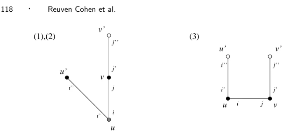
j’ j i i’ i’’ v u’ u j’’ v’ u v v’ u’ i j i’ i’’ j’ j’’ (3) (1),(2)
Fig. 1. Notations for case (1), (2) and (3) of the analysis
of the Procedure Check Edge only edges incident to u and v are traversed. More precisely:
Case (a):. v ∈ sibling(u). Then edge e = {u, v} is traversed twice and no other edges are traversed during this execution of Procedure Check Edge.
Case (b):. v ∈ pred(u). Then R traverses only edges incident to u. Let k be the greatest port number of the edges leading to a node in pred(u) and satisfying k < j. If it does not exist, set k = 0. R explores twice each edge j, j − 1, . . . , k + 1 of u, then twice edge k, and finally again twice edges k + 1, . . . , j − 1, j. To summarize, edge k of u is explored twice, and edges k + 1, . . . , j − 1, j of u are explored four times.
Case (c):. v ∈ succ(u). Then R traverses only edges incident to v. Let k be the greatest port number of the edges leading to a node in pred(v) and satisfying k < i. If it does not exist, set k = 0. R explores once edge j of u, twice each edge i − 1, i − 2, . . . , k + 1 of v, twice edge k, twice again edges k + 1, . . . , i − 2, i − 1, and finally once edge i of v (i.e., j of u). To summarize, edge i of u and edge k of v are explored twice and edges k + 1, . . . , i − 2, i − 1 of v are explored four times.
We bound now the number of times each edge e of the graph is traversed. Edge e = {u, v} is labeled i at u and j at v. Let us consider different cases (see Figure 1): (1). e = {u, v} with v = parent(u). The edge e is in the spanning tree, and thus is explored twice outside any execution of the Procedure Check Edge. During Procedure Check Edge(j) at v, edge e is explored twice. e is also explored four times during Check Edge(i) at u, except if i = 0 where e is only explored twice during Check Edge(i) at u. If there exists an edge {u′, u} labeled i′ at u and i′′
at u′ such that i′ < i and u′ ∈ pred(u), then edge e is explored twice during
Procedure Check Edge(i′) at u and twice again during Procedure Check Edge(i′′)
at u′. If there exists an edge {v′, v} labeled j′at v and j′′at v′such that j′< j and
v′ ∈ pred(v), then edge e is explored four times during Procedure Check Edge(j′)
at v and four times again during Procedure Check Edge(j′′) at v′. To summarize,
edge e is explored at most 20 times during a DFS.
(2). e = {u, v} with v ∈ pred(u) but v 6= parent(u). During Procedure Check Edge(j) at v, edge e is explored twice. e is also explored four times during Check Edge(i) at u. If there exists an edge {u′, u} labeled i′ at u and i′′ at u′ such that i′ < i
and u′∈ pred(u), then edge e is explored twice during Procedure Check Edge(i′) at
u and twice again during Procedure Check Edge(i′′) at u′. If there exists an edge
{v′, v} labeled j′ at v and j′′ at v′ such that j′ < j and v′ ∈ pred(v), then edge e
is explored four times during Procedure Check Edge(j′) at v and four times again
during Procedure Check Edge(j′′) at v′. To summarize, edge e is explored at most
18 times during a DFS.
(3). e = {u, v} with v ∈ sibling(u). During Procedure Check Edge(j) at v, edge e is explored twice. e is also explored twice during Check Edge(i) at u. If there exists an edge {u′, u} labeled i′ at u and i′′at u′ such that i′< i and u′ ∈ pred(u), then
edge e is explored four times during Procedure Check Edge(i′) at u and four times
again during Procedure Check Edge(i′′) at u′. If there exists an edge {v′, v} labeled
j′ at v and j′′at v′ such that j′< j and v′ ∈ pred(v), then edge e is explored four
times during Procedure Check Edge(j′) at v and four times again during Procedure
Check Edge(j′′) at v′. To summarize, edge e is explored at most 20 times during a
DFS.
Therefore, our exploration algorithm completes exploration in time at most 20m where m is the number of edges in the graph G.
2.2 Exploration while labeling
The above description assumes that the labeling of the graph was conducted by an external entity prior to the exploration process by the robot. As an alternative, we present here a minor change to the exploration algorithm, allowing the robot to color the graph while conducting the exploration process.
For simplicity, we assume that all nodes begin at an uncolored “blank” state, and that the robot can identify such blank nodes. Alternatively, one can assume that blank represents a forth color, making this a full 2-bit scheme. For the coloring process, the robot needs three extra bits of memory: a flag have colored and a 2-bit variable next color.
The exploration is performed in successive phases. The objective of phase i ≥ 0 is to color all nodes at distance i from r. More precisely, letting Gi be the subgraph
of the explored graph G induced by all nodes at distance at most i from the root r, the specification P (i) of phase i states that the robot starts phase i from the root, traverses all the edges of Gi, colors all blank nodes by the color next color of the
phase, and returns to the root.
At the beginning of the exploration (phase 0), the robot colors its current location white, sets next color to black, sets the flag have colored to false, and proceeds to phase 1.
For i ≥ 1, the robot’s exploration in phase i is done as described in Subsection 2.1, with the restriction that procedure Check Edge is modified as follows. Assume Check Edge is called at node u for some edge e incident to u. The procedure proceeds the same as before, except that whenever the robot traverses an edge {x, y} from a colored node x to a blank node y, the following rules are applied. —If the color of x is different from next color, then y is colored by next color,
and the procedure carries on the same way as if y was already given the color next colorwhen the robot entered it.
—Otherwise (i.e., the color of x is next color), the robot returns to x and carries on just as if the edge {x, y} did not exist.
Whenever a node is colored next color, the flag have colored is set to true. For i ≥ 1, in order to switch from phase i to phase i + 1, the robot does the following. Whenever the exploration should have stopped in the original algorithm, the robot now checks if the flag have colored is set to true, and if so, clears it, sets next color← succ(next color), and restarts the exploration (phase i + 1 starts). Otherwise, it stops.
Theorem 2.2. By the end of the execution of the modified algorithm, the graph is fully colored and the robot has explored the entire graph, terminating at the root. Proof: We have to show that the algorithm meets its specification P (i) for every i ≥ 0. Define the layer i of G as the set of nodes at distance exactly i from r. For each i ≥ 0 and time t, we say that P roperty(i) holds at time t if the specification P (i) holds and the following holds at time t.
1) All nodes of Gi are colored properly, i.e., according to the labeling L of the
previous section,
2) Only nodes of Gi are colored,
3) For i < D, next color is the color given by the labeling L to the nodes of layer i + 1.
We now prove that, at the end of phase i, P roperty(i) holds. At the end of phase 0, P roperty(0) holds by construction. For i ≥ 1, assume that at the end of phase i − 1, P roperty(i − 1) holds and let us prove that P roperty(i) holds at the end of phase i.
By the induction hypothesis, during phase i, all nodes of Gi−1 are colored
prop-erly, i.e., according to the labeling L of the previous section.
Whenever the robot colors a node u during phase i, it has arrived from a node v that is colored and whose color is not next color. Therefore, v belongs to layer i − 1, and u belongs to layer i. By the induction hypothesis, u is colored by the proper color next color.
By the modification of procedure Check Edge, whenever a non-colored node of layer i is visited by the robot coming from another node of layer i, the robot back-tracks immediately. Therefore, every time the robot reaches a node u of layer i + 1, it comes from a colored node v of layer i. Since v is properly colored next color, u is not colored, and the robot backtracks, ignoring the edge {u, v}. Informally, this means that the behavior of the robot in G at phase i is the same as its be-havior in the graph Gi at the same phase i. In fact, there is only one difference,
that occurs between siblings at layer i. In this situation, the modified procedure Check Edge backtracks and may ignore the edge. However, this has no impact on the exploration since anyway, even if all the nodes are colored a priori, the robot always backtracks when visiting a sibling.
By Theorem 2.1, during phase i, all the edges of Gi are traversed, and at the
end of the phase, the robot returns to the root. In fact, let T be the spanning tree of the explored graph G as induced by the labeling L of the previous section, and for i ≥ 0 let Ti be the subtree of T spanning all nodes at distance at most i from
layer i are visited from a node of layer i − 1, and hence are properly colored with next color. Hence specification P (i) holds.
When phase i is finished, next color is changed to succ(next color). Therefore, if i < D, at the end of phase i, the new next color is the color given by the labeling L to the nodes of layer i + 1.
Therefore, for each i ≥ 0, P roperty(i) holds at the end of phase i, and in par-ticular, the specification P (i) holds. It follows that after D phases (where D is the diameter of the graph), the robot has completed coloring all nodes of the graph and has explored the entire graph. Nevertheless, another phase is performed, in which the robot discovers that the exploration and the coloring are actually completed.
3. A 1-BIT EXPLORATION-LABELING SCHEME FOR BOUNDED DEGREE GRAPHS In this section, we describe an exploration labeling scheme using only 1-bit labels. This scheme requires a robot with O(log ∆) bits of memory for the exploration of graphs of maximum degree ∆. More precisely, we prove the following.
Theorem 3.1. For any integer ∆, there exists a robot with the property that for any graph G of degree bounded by ∆, it is possible to color the nodes of G with two colors (or alternatively, assign each node a 1-bit label) so that using the labeling, the robot can explore the graph G, starting from any given node and terminating after identifying that the entire graph has been traversed. The robot has O(log ∆) bits of memory, and the total number of edge traversals by the robot is O(∆10m).
Note, that in the case where ∆ is constant, Theorem 3.1 implies that there exists a constant memory robot and a coloring with two colors of any graph G with maximum degree ∆, such that the robot can explore G using O(m) edge traversals. To prove the theorem, we first describe a 1-bit labeling scheme L′for G = (V, E),
i.e., a coloring of each node in black or white. Then, we show how to perform exploration using L′.
Labeling L′.. As for the labeling L of the previous section, pick an arbitrary
node r ∈ V , called the root. Nodes at distance d from r are labeled as a function of d mod 8. Denote the distance between two nodes v and u in G by distG(v, u).
Partition the nodes into eight classes by letting
Ci= {u ∈ V | distG(r, u) mod 8 = i}
for 0 ≤ i ≤ 7. Node u is colored white if u ∈ C0∪ C2∪ C3∪ C4, and black otherwise.
Let
˜
C1= {u | distG(r, u) = 1}
b
C = {r} ∪ {u ∈ C2 | N (u) = ˜C1}.
Lemma 3.2. There is a local search procedure enabling a robot of O(log ∆) bits of memory to decide whether a node u belongs to bC and to ˜C1, and to identify the
class Ci of every node u /∈ bC.
Proof: Let B (resp., W) be the set of black (resp., white) nodes all of whose neighbors are also black (resp., white). One can easily check that the class C1 and
—u ∈ C6⇔ u ∈ B and there is a node in W at distance at most 3 from u;
—u ∈ C7⇔ u /∈ C6, u has a neighbor in C6, and there is no node in W at distance
at most 2 from u;
—u ∈ C1⇔ u is black, u has no neighbor in B, and u has a white neighbor v that
has no neighbor in W.
—u ∈ C5⇔ u is black, and u /∈ C1∪ C6∪ C7;
—u ∈ C3⇔ u ∈ W, and there is a node in C1 at distance at most 2 from u;
—u ∈ C4⇔ u has a neighbor in W, and there is no node in C1at distance at most
2 from u.
Based on the above characterizations, the classes C1and C3, . . . , C7can be easily
identified by a robot of O(log ∆) bits, via performing a local search. For example, the characterization of C6 is correct because of the following two observations.
First, a node in B can only belong to C6 or C7. Second, a node in C7 never has
a node in W at distance at most 3 from itself. The other characterizations can be proved similarly. Using the same ideas, the sets ˜C1and bC can also be characterized
as follows:
—u ∈ ˜C1⇔ u ∈ C1 and there is no node in C7 at distance at most 2 from u;
—u ∈ bC ⇔ N (u) ⊆ ˜C1 and every node v at distance at most 2 from u satisfies
|N (v) ∩ ˜C1| ≤ |N (u)|.
Using this we can deduce:
—u ∈ C0\ bC ⇔ u /∈ (∪7i=3Ci) ∪ C1and u has a neighbor in C7;
—u ∈ C2\ bC ⇔ u /∈ bC ∪ C1, u has a neighbor in C1 but no neighbor in C7.
It follows that a robot of O(log ∆) bits can identify the class of every node except for nodes in bC.
Proof of Theorem 3.1:
The exploration algorithm for L′follows the same strategy as the exploration
algo-rithm for L. Indeed, for u ∈ Ci we have
pred(u) = N (u) ∩ Ci−1 mod 8,
succ(u) = N (u) ∩ Ci+1 mod 8,
sibling(u) = N (u) ∩ Ci.
Therefore, due to Lemma 3.2, all instructions of the exploration algorithm using labeling L can be executed using labeling L′, but for the cases not captured in
Lemma 3.2, i.e., bC.
To solve the problem of identifying the root, we notice that each of the nodes in bC can be used as a root and all the others can be considered as leaves in C2,
without changing the classes of the nodes not belonging to bC. Thus, when leaving the root, the robot memorizes the port p by which it should return to the root. When the robot leaves a node u ∈ ˜C1 through port p, it leaves it in the up state
and deletes the content of the variable storing p. Then, on the reached node v, the robot acts as if v would be in the class C0 (which is the case since v is the root),
leaves a node u ∈ ˜C1 through a port different from p, and reaches a node in bC, it
leaves it in the down state and then acts as if the reached node would be in the class C2, i.e., it comes back to u in the up state.
If the exploration begins at the root, then the above is sufficient. To handle explorations beginning at an arbitrary node, it is necessary to identify the root. Since every node in bC can be used as a root, it suffices to find one node of bC by going up, and then start the exploration from it as described above.
It remains to compute the number of edge traversals performed by the robot during the exploration. The only edge traversals performed by the robot using L′ but not performed by the robot using L are the edge traversals performed by
the robot during the local search procedure enabling the robot to identify the class of the current node. Thus, the total number of edge traversals performed by the robot considered in this section is at most O(f (∆)m), where f (Delta) is the maximum number of edge traversals performed during the execution of the local search procedure.
The fact that f (Delta) = O(∆10) follows by observing that the local search
procedure can be decided by inspecting the neighborhood of the node up to distance 10. Indeed, the membership of a node in sets C6, C7, C1, C5, C3, C4, ˜C1, bC, C0\ bC,
and C2\ bC can be decided by inspecting the neighborhood of this node up to
distance, respectively, 4, 5, 3, 5, 5, 5, 7, 10, 6, and 10.
We note that the bound on the total number of edge traversals can possibly be reduced further, using the following observation: once the robot has computed the class of the current node v using the described local search procedure, the class of any neighbor of v can only take three identified values. In this case, the robot can use a simplified procedure to identify the class of any subsequently visited node.
4. IMPOSSIBILITY RESULTS
In this section we aim to prove some bounds on exploration by robots with no memory, i.e., single state robots. We present two such bounds, one for exploring graphs with self loops (loops connecting a node to itself) and one for simple graphs, containing no self loops. We assume the robots are stateless and therefore the port traversed by the robot depends only on the color and the degree of the current node and of the label of the port by which the robot arrived at this node (unless the node is the starting node, in which case the port traversed depended only on the node’s color and degree).
We aim to construct a graph (with self loops) that cannot be explored by a 1-state robot. The constructed graph will be a star-like graph with the middle node having degree d, where some of its ports lead to degree one nodes while others loop back into the middle node. We will show that an adversary, that is given the details of the robot’s transition table for each of c ≤ d/2 − 1 colors, can construct such a graph which can not be explored by this robot. The proof relies on arguing that at least one node will not be explored for every possible coloring of the central node. We begin by several definitions that will help us construct such a graph.
Recall that when a 1-state robot enters a degree-d node v by port i, it will leave v by port j where j depends only on i, d and the color c of v. Thus for fixed d, each
color corresponds to a mapping from entry ports to exit ports, namely, a function from {0, 1, · · · , d − 1} to {0, 1, · · · , d − 1}. Partition the functions corresponding to the colors of nodes of degree d into surjective functions f1, f2, · · · , ft and
non-surjective functions g1, g2, · · · , gr. We have 0 < t + r ≤ d/2 − 1. Let ci be the color
corresponding to fi, and ct+i be the color corresponding to gi. For each gi, choose
pito be some port number not in the range of gi. Since for each i, pi is not in the
range of gi, starting from a node colored by ct+i the robot will never traverse port
pi.
To show that the central node can not be colored by any of the colors ci, 1 ≤ i ≤ t
(the colors with a surjective transition function) a graph should be constructed in which coloring the central node by any of these colors will result in at least one of the leaves not being explored. To do that we construct a family {G0, G1, · · · , Gt}
of graphs such that, for every k ∈ {0, 1, · · · , t}:
(1) Gk has exactly one degree-d vertex v (possibly with loops);
(2) all edges are either loops incident to v, or edges leading from v to some degree-1 node;
(3) edges labeled p1, p2, · · · , pr at v (if any, i.e., if r > 0) are not loops (and thus
lead to degree-1 nodes);
(4) the edge labeled p0 leads to some distinguished degree-1 node, denoted by u0;
(5) there exists a set Xk ⊆ {0, 1, · · · , d − 1} such that {p0, p1, · · · , pr} ⊆ Xk and
d − |Xk| > 2(t − k), and for which, in Gk, edges with port number not in Xk
lead to degree-1 vertices.
For a given graph Gk−1, we define the following: For a port i ∈ {0, 1, · · · , d − 1},
set twin(i) = j if there exists a port j and a loop labeled by i and j in Gk−1; Set
twin(i) = i otherwise. This definition of twin corresponds to the port by which the robot reenters the central node after leaving it using port i; if port i leads to a leaf then the robot returns from the leaf to the central node using the same port, and if port i leads to a loop returning through port j, the robot immediately reenters the central node through port j.
We prove the following property for any k = 0, · · · , t: PropertyPk.
In Gk, if the color of v is in {c1, · · · , ck}, then the robot, starting at u0 ∈ V (Gk),
cannot explore Gk. More precisely any vertex attached to v by a port 6∈ Xk is not
visited by the robot.
The proof relies on starting with a star graph, and for each color, k, replacing two nodes by a loop (if needed). The loop is formed between appropriate ports, chosen such that the robot will return to previously visited ports without completing the exploration of all ports.
Lemma 4.1. For every k = 0, . . . , t there exists a graph Gk, having property Pk. Proof: We prove the lemma by induction on k. First, note that Property P0 is
trivially true for every graph. Still, to ease the induction proof, we would like to define the graph G0 and the set X0. Let G0 be the star composed of one
degree-d vertex v and d leaf vertices. Let p0 ∈ {0, 1, · · · , d − 1} \ {p1, p2, · · · , pr}
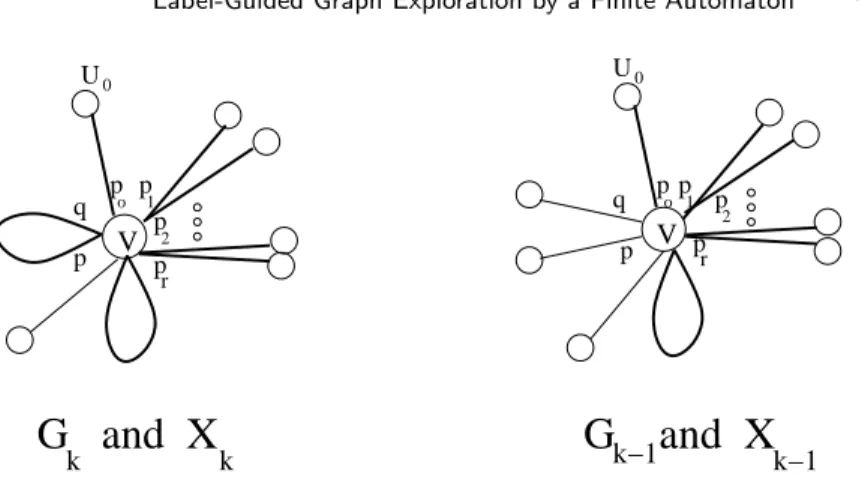
V V 2 q p p 2 p p p p q pp1 p o o r r k
G and X
k−1G and X
k−1 k 1 p 0 U U0Fig. 2. In the right figure, the thick lines correspond the ports in Xk−1. Port p is the first port not in Xk−1that is visited by the robot at v, assuming that the starting node in u0 and that v is colored with color ck. Port q is that port ih, where h is the smallest such that ih∈ Xk/ −1. In Gk, Ports p and q (if they are different) are connected, constructing a loop, as depicted in the left figure. Xkthen becomes Xk= Xk−1∪ {p, q}.
t + r ≤ d/2 − 1. Thus, t ≤ d/2 − 1 and hence 2t + r + 1 ≤ d − 1. Therefore, we have d − |X0| = d − (r + 1) > 2t.
Let k > 0, and let Gk−1 and Xk−1 be respectively a graph and a set satisfying
the induction property for k − 1. Assume first that v is colored by color ck and
that the robot starts its traversal at u0. If the robot never visits vertices attached
to v by ports not in Xk−1 then the graph Gk−1 and the set Xk−1 satisfy Pk. I.e.,
Gk= Gk−1and Xk= Xk−1. Otherwise, let p be the first port not in Xk−1 that is
visited by the robot at v, when starting at u0.
Define a sequence of ports (il)l≥1 as follows. Let i1 be the port in Xk−1 such
that fk(i1) = p. For all l ≥ 2, let il be the port such that fk(il) = twin(il−1).
This sequence is well defined because fk is surjective. The sequence represents (in
reverse order) the ports spanned by the robot on its exploration process towards port p.
Observe that there exists some l such that il ∈ X/ k−1. Indeed, suppose, for
the purpose of contradiction, that il ∈ Xk−1 for all l. Since Xk−1 is finite, there
exists some il = il+m for m ≥ 1. Let il be the first port repeated twice in this
process. If l > 1, then we have fk(il) = twin(il−1) and fk(il+m) = twin(il+m−1).
Therefore twin(il−1) = twin(il+m−1), yielding il−1 = il+m−1 by bijectivity of fk,
which contradicts the minimality of l. If l = 1, then we have i1 = i1+m, therefore
im= p, contradicting ij ∈ Xk−1 for all j.
From the above, let h be the smallest index such that ih∈ X/ k−1. Let q = ih. If
q = p, then set Gk = Gk−1 and Xk = Xk−1∪ {p}. If q 6= p, then connect ports p
and q to create a loop, denote the new graph Gk and let Xk = Xk−1∪ {p, q}. See
Figure 2.
In Gk, if v is colored by color ck, then by the choice of p, starting at u0, the
robot enters and exits v through ports in Xk−1 until it eventually exits v through
port p. After that, the robot goes back to v by port q. Port q was chosen so that it causes the robot to continue entering v on ports ih−1, ih−2, · · · i1, after which the
of v occurring in this cycle are all from Xk, the robot does not visit any of the
ports outside Xk, as claimed. By induction, we have d − |Xk−1| > 2(t − (k − 1)).
By the construction of Xk from Xk−1, we have |Xk| ≤ |Xk−1| + 2. Therefore
d − |Xk| > 2(t − k), which completes the correctness of Gk and Xk.
If the color of v in Gk is in {c1, · · · , ck−1} then the robot is doomed to fail in
exploring Gk. Indeed, since starting at u0in Gk−1the robot does not traverse any
of the vertices corresponding to ports not in Xk−1, then in Gk too, the robot does
not traverse any of the vertices corresponding to ports not in Xk⊇ Xk−1, and thus
fails to explore Gk because d − |Xk| ≥ 1. This completes the proof of Pk and thus
the induction.
Theorem 4.2. For any d > 4, and for any 1-state robot using at most d/2 − 1 colors, there exists a graph (with loops) with maximum degree d and at most d+1 vertices that cannot be explored by the robot.
Proof: Fix d > 4, and assume for contradiction that there exists a 1-state robot exploring all graphs of degree d colored with at most d/2 − 1 colors. By Lemma 4.1, Gt has property Pt and thus at least one of its vertices is not explored by the
robot if the node v is colored with a color in c1, c2, · · · , ct. If v is colored ct+i with
1 ≤ i ≤ r, then assume that the robot starts the traversal at vertex u0. Since the
edge labeled pileads to a degree-1 vertex in Gt, this vertex will never be visited by
the robot, by definition of pi. Therefore the graph Gt cannot be explored by the
robot.
The theorem above makes use of graphs with loops. For graphs without loops we use the same construction, replacing loops with simple subgraphs without loops. However, in a loop, a robot entering the loop through one port will immediately return to its last visited node through the other port. If the loop is replaced by a more complex structure we need to guarantee that the robot will necessarily return to the node from which it entered this structure using the second port connected to this structure.
Consider a node w of degree d, accessible from the rest of the graph through two ports, p and q, and all its other d − 2 ports lead to leaves. We aim to show that there exists a labeling of the two ports, such that entering the node through one of them, will guarantee leaving through the other, regardless of the color used for the node. As before we define the set {p1, · · · , pr} of ports excluded from non-surjective
colors and have each of them lead to a leaf. We also note, that by looking at each function fias a permutation on d elements, if for some fi, the cycle decomposition
of this permutation consists of more than two cycles, then w cannot be colored by fi because whatever ports p and q are chosen, the robot can visit only ports
corresponding to the cycles that p and q belong to. Therefore we may assume that the cycle decomposition of each of the relevant fi consists of at most two cycles.
We will term such a color (whose function is surjective and contains at most two cycles) as useful.
Using the next two lemmas we show that for high enough degree d, we can always choose two ports p, q /∈ {p1, · · · , pr} such that for every useful color they belong to
Lemma 4.3. Given the functions f1, · · · , fk of k useful colors, there exist at least d/2k ports that are in the same cycle for each of the k functions.
Proof: We prove by induction on k. For k = 1, f1 contains at most two cycles
permuting the d ports, therefore one of these cycles contains at least d/2 ports. Assume that the induction hypothesis is true for k = n, i.e., there are s ≥ d/2n
ports that are in the same cycle for each of f1, · · · , fn. Now, fn+1contains at most
two cycles, so one of them contains at least half of the s ports. Therefore, there are at least s/2 ≥ d/2n+1 ports that belong to one cycle in each of the n + 1 functions,
completing the induction.
Lemma 4.4. For any d > 4 and for c ≤ ⌊log d⌋ − 2 colors, there exists at least two ports p, q ∈ {0, 1, · · · , d − 1} \ {p1, p2, · · · , pr} that belong to the same cycle for
all useful colors.
Proof: Assume that there are k ≤ t useful colors, by Lemma 4.3 there are at least d/2k ports belonging to the same cycle for all useful colors. Now d/2k ≥ d/2t≥
22+c−t = 22+r= 4 · 2r. Therefore, there are at least 4 · 2r ports belonging to one
cycle for all useful colors, and 4 · 2r≥ 2 + r for all r ≥ 0. Thus, p and q can always
be selected to be other than p1, p2, · · · , pr.
We now turn to the main theorem, building on the construction with loops of Theorem 4.2 presented above, and replacing the loops by paths in the graph.
Theorem 4.5. For any d > 4 and for any 1-state robot using at most ⌊log d⌋ − 2 colors, there exists a graph of maximum degree d, without loops, that cannot be explored by the robot.
Proof: As in the proof of Theorem 4.2, denote the functions corresponding to the colors by f1, f2, · · · , ft, g1, g2, · · · , grwhere the fi’s are surjective functions and the
gi’s are non-surjective ones. For each gi, choose pi to be some port number not in
the range of gi. We use the same proof as for Theorem 4.2, except that we replace
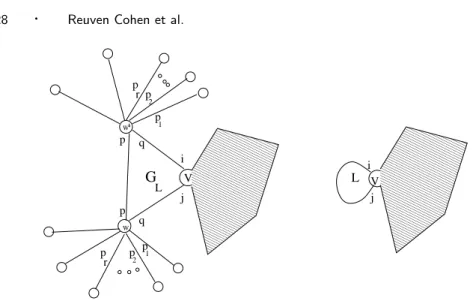
each loop L of the construction in there by a loopless graph. For a loop L of vertex v, with port numbers i and j, let GL be the following graph. (See Figure 3.)
Connect v by edges to two new vertices w and w′, add the edge (w, w′), and connect
w (respectively, w′) to d − 2 new vertices n
1, n2, · · · , nd−2 (resp., n′1, n′2, · · · , n′d−2).
We now set the port numbering for GL. Assign the port numbers i and j for the
edges (v, w) and (v, w′). At w (respectively, w′) use the port numbers p
1, p2, · · · , pr
for the edges (w, n1), (w, n2), · · · , (w, nr) (resp., (w′, n′1), (w′, n′2), · · · , (w′, n′r)). The
port numbers p and q that w uses for the edges (w, v) and (w, w′) are the same as
the port numbers that w′ uses for the edges (w′, v) and (w′, w). They are chosen
to be in the same cycle for all useful colors, as shown in Lemma 4.4.
We immediately get that w and w′ cannot be colored by a color whose
corre-sponding function is in the set g1, g2, · · · , grsince these functions are not surjective
and ports {p1, p2, · · · , pr} lead to leaves of w and w′. Also, w and w′ cannot be
colored by a non-useful color, since it contains at least three cycles, and since w and w′ can only be entered through two ports (p and q) all ports belonging to cycles
not containing p and q will not be visited.
Therefore, w and w′ must be colored by a useful color. However, for all useful
V 000000000 000000000 000000000 000000000 000000000 000000000 000000000 000000000 000000000 000000000 000000000 000000000 000000000 000000000 000000000 000000000 000000000 000000000 000000000 000000000 000000000 000000000 000000000 000000000 000000000 111111111 111111111 111111111 111111111 111111111 111111111 111111111 111111111 111111111 111111111 111111111 111111111 111111111 111111111 111111111 111111111 111111111 111111111 111111111 111111111 111111111 111111111 111111111 111111111 111111111 000000000 000000000 000000000 000000000 000000000 000000000 000000000 000000000 000000000 000000000 000000000 000000000 000000000 000000000 000000000 000000000 000000000 000000000 000000000 000000000 000000000 000000000 000000000 000000000 000000000 000000000 111111111 111111111 111111111 111111111 111111111 111111111 111111111 111111111 111111111 111111111 111111111 111111111 111111111 111111111 111111111 111111111 111111111 111111111 111111111 111111111 111111111 111111111 111111111 111111111 111111111 111111111 L G L W W’ i j j i q p q p p p p p p 1 1 2 2 p r r V
Fig. 3. The loop L (with ports i and j) in the right figure, is replaced by the subgraph GL, as depicted in the left figure. Ports p and q are chosen such that {p, q} ∩ {p1, p2, · · · pr} = ∅ and such that they belong to the same cycle, for every useful color. It follows that if the robot exits v through port i, it must return to v via port j, and vice versa.
must leave through q and vice versa. It follows that whenever the robot enters GL
from v in port i it must return to v in port j (and vice versa). Therefore, the loop L in the proof of Theorem 4.2 can be replaced by GL.
5. DISCUSSION
It was known that there is no 0-bit exploration-labeling scheme, even for bounded degree graphs. We proved that there is a 2-bit exploration-labeling scheme for arbitrary graphs, and that there is a 1-bit exploration-labeling scheme for bounded degree graphs. It remains open whether or not there exists a 1-bit exploration-labeling scheme for arbitrary graphs.
REFERENCES
BLUM, M. AND KOZEN, D. 1978. On the power of the compass (or, why mazes are easier to search than graphs). In 19th Symposium on Foundations of Computer Science (FOCS), 132–142.
BUDACH, L. 1978. Automata and labyrinths. Math. Nachrichten, 195–282.
DIKS, K., FRAIGNIAUD, P., KRANAKIS, E., AND PELC, A. 2004. Tree Exploration with Little Memory. Journal of Algorithms 51 (1), 38–63.
FRAIGNIAUD, P., ILCINKAS, D., PEER, G, PELC, A. AND PELEG, D. 2005. Graph Explo-ration by a Finite Automaton. Theoretical Computer Science 345 (2-3), 331–344.
FRAIGNIAUD, P., ILCINKAS, D., AND PELC, A. 2006. Oracle size: a new measure of diffi-culty for communication tasks. In Proc. the 25th Annual ACM Symposium on Principles of Distributed Computing (PODC).
FRAIGNIAUD, P., ILCINKAS, D., RAJSBAUM, S., AND TIXEUIL, S. 2005. Space lower bounds for graph exploration via reduced automata. In Proc. 12th Int. Colloq. on Structural Informa-tion and CommunicaInforma-tion Complexity (SIROCCO), 140–154.
FRAIGNIAUD, P., KORMAN, A., AND LEBHAR, E. 2007. Local MST Computation with Short Advice. In Proc. 19th ACM Symp. on Parallelism in Algorithms and Architectures (SPAA). GASIENIEC, L, PELC, A, RADZIK, T, AND ZHANG, X. 2007. Tree exploration with
loga-rithmic memory. In proc. 18th Annual ACM-SIAM Symp. on Discrete Algorithms (SODA), 585–594.
KORMAN, A., KUTTEN, S., AND PELEG, D. 2005. Proof Labeling Schemes. In Proc. the 24th Annual ACM Symposium on Principles of Distributed Computing (PODC).
KOZEN, D. 1979. Automata and planar graphs. Fundamentals of Computation Theory (FCT), 243–254.
RABIN, M.O. 1967. Maze threading automata. In a Seminar talk presented at the University of California at Berkeley.
ROLLIK, H.A. 1980. Automaten in planaren Graphen. Acta Informatica 13, 287–298.
SHANNON, C.E. 1951. Presentation of a maze-solving machine. In 8th Conf. of the Josiah Macy Jr. Found. (Cybernetics), 173–180.