Contributions to the analysis and mitigation of liquefaction in loose sand slopes

(1)

Contributions to the Analysis and Mitigation of

MASSACHU: vS iNOITrfT

Liquefaction in Loose Sand Slopes

Antonios Vytiniotis

Master of Science in Civil Engineering (2009), Massachusetts Institute of Technology, Department of Civil and Environmental Engineering

Diploma in Civil Engineering (2005), National Technical University of Athens, Department of Civil Engineering

N

('

>-October

28, 2011

Certified by

Andrew

J.

Whittle Professor of Civil and Environmental Engineering

IThts

upervi4r

Accepted by

Heidi M. Nepf Chair, Departmental Committee for Graduate Students

(2)

(3)

Contributions to the analysis and mitigation of

liquefaction in loose sand slopes

Antonios Vytiniotis

Submitted to the Department of Civil and Environmental Engineering on October 28, 2011, in Partial Fulfillment of the Requirements for the Degree of Doctor of Philosophy in the field of

Civil and Environmental Engineering

Abstract

This research analyzes the vulnerability of loose granular waterfront fills to liquefaction in seismic events and considers the effectiveness of Pre-fabricated Vertical (PV) drain systems in mitigating potential damage. The analyses are based on non-linear finite element simulations of coupled flow and deformation using the OpenSees open-source software framework. The analyses make extensive use of an advanced elasto-plastic model developed by Dafalias and Manzari (2004; DM2004) for simulating the cyclic response of sand. The model formulation is based on theories of bounding surface plasticity and critical state soil mechanics. The thesis presents a series of algorithms needed to achieve robust integration of the DM2004 model in OpenSees, documents model calibration for two test sands (Nevada, Toyoura), and evaluates its predictive capabilities and limitations at the element level. The results show that although the DM2004 model describes quite realistically the accumulation of plastic shear strains in drained and undrained cyclic shearing, the material can shakedown to a stable condition over a large number of load cycles (a condition of alternating plasticity). One-dimensional drain elements have been developed to represent laminar or turbulent discharge through the PV drains based on classic Darcy-Weisbach pipe flow. The elements also allow for fluid storage for cases where the PV drains extend through low permeability clay soils above the water table. The numerical predictions of ground response have been evaluated using results from a

well-instrumented centrifuge model test (SSK01) performed by colleagues at the University of California at Davis (Kamai et al., 2008). The model includes a full array of PV drains installed within one of two facing slopes (directed towards a central channel) under a series of harmonically-varying horizontal base acceleration events. The simulations show reasonable predictions of accelerations, pore pressure accumulation and displacements within the untreated loose Nevada sand fill and the effectiveness of the PV drains in reducing permanent deformations within the slope.

(4)

Numerical simulations of vulnerable piled-wharf structures have been carried out for the reference geometry of an 18m high, partially submerged fill slope (typical of port facilities on the USA West coast). This thesis describes the free-field simulations of ground response for a

suite of 58 reference seismic ground motions from the NGA database (Chiou et al., 2008) and from Shakeout simulations (Graves et al., 2008) while a parallel study at the Georgia Institute of Technology (Shafieezadeh, PhD 2011) couples the predicted free-field pore pressures and ground deformations to the response of the piled-wharf structure.

The numerical framework for free-field analyses involves special considerations of the boundary conditions to minimize the reflection of energy from far-field lateral boundaries and to represent mechanical and hydraulic interactions at the ocean-soil interface. The analyses use the DM2004 model with input parameters corresponding to Toyoura sand, and include parametric studies to evaluate how the in-situ fill density and hydraulic conductivity affect the ground response for a reference strong motion acceleration record. Numerical simulations have been performed for the suite of 58 reference ground motions for both the untreated (i.e., existing) fill and for the case where full-depth PV drains are installed at locations behind the crest of the slope (i.e., minimally-intrusive mitigation system). The computed permanent slope deformations are not well described by published empirical correlations, but are well correlated with the peak ground accelerations (PGA) and especially the Arias intensity (Ia), while directionality of the ground motions has minimal effects on the ground response. More detailed observations show that average shear strains (i.e., slope damage) are closely linked to the development of excess pore pressures within the slope. The PV drain mitigation system is effective in reducing permanent deformations and achieves an improvement ratio in the range

1.5-3.0 (untreated: PV deformations) that is insensitive to the ground motion characteristics.

The damage results have been incorporated in slope fragility curves that can be used by risk analysts to quantify the expected costs from earthquake damage.

Thesis Supervisor: Andrew J. Whittle

(5)

Acknowledgements

First and foremost I would like to thank my advisor Prof. Andrew J. Whittle for all his help in transforming me into a researcher, and helping me understand geotechnical engineering. Also, I want to thank him for his industrious efforts to make this document academically readable. I would like to thank my co-advisor Prof. Eduardo Kausel for his invaluable help in understanding soil dynamics, and trusting me to lecture part of his classes. Finally, I would like to thank Prof. Lallit Anand for helping me see the bigger picture of my research.

During this PhD there are so many people that helped me enormously in all the phases of this journey, and I would like to thank. Thanks Miriam. Stella, Nina, Despina, Giorgos, Gerasimos,

Eliza, Roula, Gonzalo, Eleni, Stavronikos, Kostas, Yannis, Nikos. Many of you opened my eyes, helped me stand on my feet, and definitely without you I wouldn't have survived the PhD life. Thank you!

Special thanks to my climbing mates Nikolas, Shoshanna, Nikolas, Alina and Ruben. To my friends from the office Sherif, Kartal, Anna. Many thanks to Dr Lucy Jen for all the coaching in my pre and post academic life.

Also, thanks to Vasilis for keeping cool with my crazy schedule the last year. Thanks to Adonis for keeping my crazy self there.

I like to thank my brother Dimitris for the family dinners we had in Philly, that made me feel I

was still not far away from home, no matter the ocean separating me and my family, and my parents for all the times they had to travel overseas to see me. Hope there are more times like this to come.

Thanks to NSF grant CMS-0530478 and the Alexander Onassis public benefit foundation for the financial support for this research.

But I would really like to dedicate this thesis to my grandfather, Antonis Moutafis, for his unconditional love and care for me are in part responsible for the person I am today.

(6)

(7)

Table of Figures

Figure 1-1 Seismic hazard for western USA by USGS (PGA with 2% probability of exceedance in

5 0 y e a rs)... 3 1

Figure 1-2 Seismic hazard for central/eastern USA by USGS (PGA with 2% probability of

excee d ance in 50 years)... 3 1

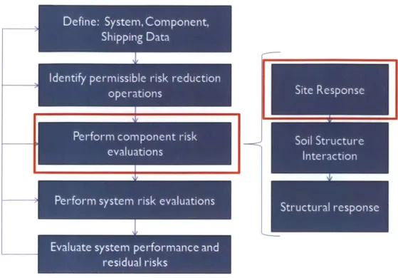
Figure 1-3 Seismic risk mitigation project overview. In red squares are shown the parts of the project perform ed in this research... 32

Figure 1-4 Typical soil-foundation-structural system for pile supported wharf (Ivey, 2010) ... 32

Figure 1-5 (a) Cross-section of casing and PV-drain (Pestana et al., 1997) and (b) Side view of a ty pical PV -d rain ... 3 3

Figure 1-6 Typical installation of PV-d rains from drilling equipment... 33 Figure 1-7 Various observed modes of pile failure in liquefiable soils (Tokimatsu et al, 1996)... 34 Figure 2-1 Forces acting on a triangular failing wedge under pseudostatic accelerations av and ah ... 6 3 Figure 2-2 Acceleration profiles in a: (a) rigid Slope; and (b) flexible Slope... 63 Figure 2-3 Liquefaction mitigation though the use of earthquake drains. The storage capacity of th e d ra in s is illu strate d . ... 6 3

Figure 2-4 PV-drain installation geometries and equivalent drain spacing for rectangular and tria n g ula r a rray s... 6 4

Figure 2-5 Drainage during a seismic event; simplified model used in the Seed & Booker (1977) and O noue (1988) analyses. ... 64 Figure 2-6 Pore pressure generation from undrained direct simple shear tests: data range and fitted m odel for 0=0.7 (DeAlba et al., 1975)... 65

Figure 2-7 Design charts for groups of gravel drains against liquefaction (Seed & Booker, 1977).

... 6 5

Figure 2-8 Effect of well resistance on developed excess pore pressures (Onoue, 1988)... 66 Figure 2-9 Vertical Section of the idealization of a PV-drain, consisting of an outer core with horizontal flow and an inner core with vertical flow ... 66

Figure 2-10 Effect of drain storage capacity and well resistance on control of excess pore

pressure (Pestana et al., 1997). ... 67

Figure 2-11 Illustration of a water saturated soil sample showing the soil skeleton and the water

... 6 7

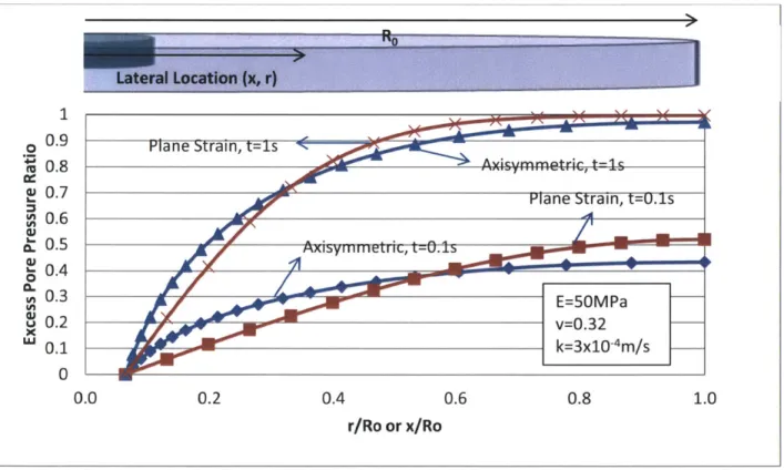
Figure 2-12 Equivalence of axisymmetric to plane strain models for the case where the drain spacing (n = de/dw) is the same in the 3D and in the plane strain model (after Hird et al., 1992)68

(12)

Figure 2-13 Comparison of 3D and 2D excess pore pressure distribution using the matching procedure of Hird et al. (1992) for a vertical applied consolidation load (performed using

AAUTM

ABAQU ST; Vytiniotis, 2009) ... 68

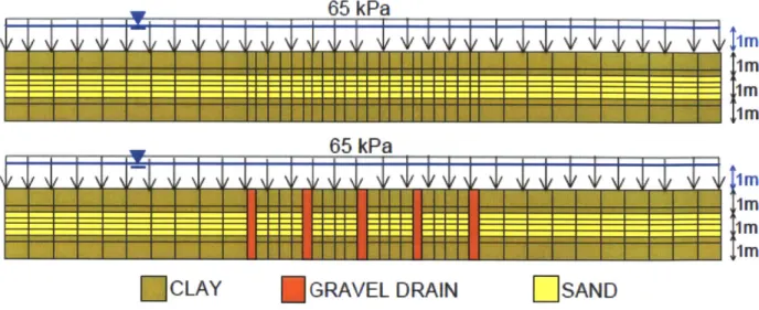
Figure 2-14 Treated and untreated soil profile simulated by Papadimitriou et al. (2007) ... 69

Figure 2-15 Excess Pore Pressure measured in the sand layer for different improvement ratios (dw/de) under a harmonic sinusoidal basal acceleration (amax=0.4_{g, T=0.3s), Papadimitriou et al.}

(2 0 0 7 ) ... 6 9

Figure 2-16 Illustration of a fragility curve ... 70

Figure 2-17 Probabilistic demand models for (a) pile deck connections, (b) pile sections, (c) relative movement of the wharf with respect to the landside crane rail ... 70

Figure 2-18 W harf and Landline Rail Configurations... 71 Figure 2-19 Seismic Fragility Curves for slight, moderate, and extensive damage states for (a) pile-deck connections, (b) pile sections, (c) relative movement of the wharf with respect to the la n d slid e cra n e rail ... 7 1

Figure 3-1 Limiting Compression Curve and Critical State Line (Conceptual model after Pestana

& W h ittl e , 19 9 9 ) ... 1 14

Figure 3-2 Sand shear deform ation m echanism s ... 115

Figure 3-3 Drained triaxial shear tests for dense and loose Sacramento River sand (Dr=100% and D r=38% respectively) (Lee, 1965)... 116

Figure 3-4 Undrained triaxial shear tests for loose and dense Toyoura sand (Dr=1 6_{% and Dr=6}4_% respectively) (Ishihara, 1996)... 117

Figure 3-5 Measured critical state line for Toyoura sand from undrained triaxial compression d ata (Ish ih a ra, 19 9 3)... 1 18

Figure 3-6 Definition of secant shear modulus, Gsec, and damping ratio (... 118

Figure 3-7 Experimental data for the: (a) degradation of G/Gmax vs. yc (b) { vs. yc curves for dry Toyoura sand (Data after Kokusho, 1980) ... 119

Figure 3-8 Typical undrained shear behavior of sand in constant volume DSS test (Dense Nevada Sand, Dr=77%, av=77kPa, CSR=0.36; Kammerer et al., 2002)... 120

Figure 3-9 Cyclic stress ratio for liquefaction of Toyoura sand within 20 cycles of loading for different initial relative densities (Tatsuoka et al., 1986b)... 121 Figure 3-10 Number of cycles to cause initial liquefaction for Toyoura sand (Hosono &

Y o sh im in e, 2 0 0 4 ) ... 1 2 1

Figure 3-11 Effect of confining stress on the cyclic strength of sands ... 122 Figure 3-12 Yield, bounding, dilatancy, and critical state surfaces in triaxial space (for @<O) .. 122

Figure 3-13 Schematic diagram of the yield, critical, dilatancy, and bounding surfaces used in the DM 2004 m odel shown on the n plane (for 0<0)... 123

(13)

Figure 3-14 Schematic diagram of DM2004 predictions of an undrained triaxial compression test in a loose and a dense sand ... 124 Figure 3-15 Calibration of critical state line with experimental undrained triaxial compression d ata fro m Ishihara (1993) ... 125

Figure 3-16 Calibration of small strain elastic stiffness from drained triaxial compression tests on isotropically consolidated Toyoura sand. Data after Verdugo and Ishihara (1996), Miura

(1979), and M iura et al. (1984)... 126

Figure 3-17 Comparison of numerical simulations (DM2004) vs. experimental measurements (Verdugo and Ishihara, 1996) of drained triaxial shearing of Toyoura sand at p'o=500kPa ... 127

Figure 3-18 Comparison of numerical simulations (DM2004) vs. experimental measurements (Verdugo and Ishihara, 1996) of drained triaxial shearing of Toyoura sand at p'o=1OOkPa ... 128

Figure 3-19 Comparisons of simulated and measured response for monotonic undrained simple shearing of Toyou ra sand ... 129

Figure 3-20 Comparison of the predictions of the DM2004 model vs. experimental data for the: (a) degradation of G/Gmax vs. y (b) vs. y curves for dry Toyoura sand. Data from triaxial cyclic shearing apparatus (Kokusho, 1980) ... 130

Figure 3-21 Predictions of the DM2004 model for the: (a) degradation of G vs. yc (b) ( vs. yc

curves for dry Toyoura sand. ... 131

Figure 3-22 DM2004 Model simulation of two-way undrained cyclic simple shearing test at

Dr=30% , Tc/a''vo=0.1, 0.2, 0.4 and To/a'vo=0.0 ... 132

Dr=40% , c/a'Yo=0.1, 0.2, 0.4 and To/a',o=0.0 ... 133

Figure 3-24 DM2004 Model simulation of two-way undrained cyclic simple shearing test at

Dr=50% , Tc/cy'vo=0.1, 0.2, 0.4 and To/a',vo=0.0 ... 134

Dr=40% , Tc/ y'vo=0.1, 0.2, 0.4 and To/a'vo=0.2 ... 135

Figure 3-26 Number of cycles to reach alternate plasticity behavior in undrained cyclic simple shearing, for different relative densities and different applied cyclic shear stress ratios

(o'vo=100kPa). Next to each point the double amplitude shear strain at the alternate plasticity stage of load ing is reported... 136

Figure 3-27 Comparison of experimental vs. simulated results of undrained cyclic triaxial

shearing test, Dr=45% (e=0.808). Data after Ishihara et al. (1975). ... 137

shearing test, Dr=62% (e=0.743). Data after Yoshimine & Hosono (2000) ... 138

(14)

Figure 3-30 Double amplitude shear strain contours produced by CKOUDSS simulations of

Toyoura Sand using the DM 2004 soil m odel ... 140 Figure 3-31 Comparisons of simulated (DM2004) and measured (Hosono & Yoshimine, 2004) liq uefactio n curves... 14 1

Figure 3-32 Calibration of small strain stiffness at Dr=40% (Data after Arulmoli, 1992) ... 141 Figure 3-33 Critical State Line Calibration (Data after Arulmoli, 1992)... 142 Figure 3-34 Calibration of ho with undrained triaxial compression tests for Nevada sand at

D r= 4 0 % ... 14 3

Figure 3-35 Calibration of Ao parameter using constant volume DSS tests for Nevada sand at

D r= 4 0 % ... 14 4

Figure 3-36 Calibration of c' and Zmax parameters using constant volume DSS tests for Nevada sa n d at D r= 5 0 % ... 14 5

Figure 3-37 Calibration through undrained triaxial shearing at Dr=40% (Data after Arulmoli,

1992). The second two columns of the figure plot exactly the same simulation and experiment,

but they blow it up in order to examine the calibration at small strain levels. ... 146

Figure 3-38 Calibration through undrained triaxial shearing at Dr=60% (Data after Arulmoli,

1992). The second two columns of the figure plot exactly the same simulation and experiment,

but they blow it up in order to examine the calibration at small strain levels. ... 147 Figure 3-39 Numerical simulation vs. measured experimental results for Dr=4 0_{% (Data after} C o rral , 2 0 0 6 ) ... 14 8

Figure 3-40 Numerical simulation vs. measured experimental results for Dr=6_{8% and 50% (Data} after Kam m erer et al., 2000) ... 149 Figure 4-1 Moody Diagram: Estimation of the Darcy friction factor (X) for different Reynolds n u m b e r... 2 0 4

Figure 4-2 Coordinates, pressure, flow, force, and displacement definitions for the uncoupled d ra in e le m e nt... 2 0 4

Figure 4-3 Various regimes and definitions used to integrate the Darcy-Weisbach equation for fully tu rb ule nt flo w ... 20 5

Figure 4-4 Illustration of the storage capacity effect mechanisms ... 206

Figure 4-5 Flowchart of forward Euler explicit integration procedure... 207 Figure 4-6 Stress paths and stress-strain curves using the original explicit forward Euler

Integration scheme for three different Gauss points in a finite element analysis with the

D M 20 0 4 m o d el ... 20 8

Figure 4-7 Flowchart of automatic sub-incrementation scheme for the DM2004 soil model... 209 Figure 4-8 Illustration of return-to-apex correction for the DM2004 soil model in an effective stress space. If after the explicit integration step the stress state has tensile components of

(15)

normal stress (i.e., one case could be when p'<0), then the stress state is returned to a stress

state inside the yield surface very close to its apex. ... 210

Figure 4-9 Flowchart of return to apex scheme for the DM2004 soil model ... 210

Figure 4-10 Illustration of return-to-bounding/critical state surface correction for the DM2004 soil model in an effective stress space. If after the explicit integration step the stress state Y' +1 lies outside the bounding or critical state surface (whichever is largest) the return-to-bound ing/critical state surface algorithm is invoked. The stress state is returned to the bounding/critical state surface at point o'r'i1 using a closest projection path... 211

Figure 4-11 Flowchart of the return-to-bounding/critical state surface algorithm for the DM2004 soil model. A value of tolerance, ftoI=1x10-, has been used throughout this research. ... 2 1 2 Figure 4-12 Flowchart of the implemented DM2004 model integration procedure. In red boxes we illustrate three important algorithms implemented, the sub-incrementation algorithm, the return-to-apex algorithm, and the return-to-bounding/critical state surface... 213

Figure 4-13 Stress paths and stress-strain curves using the explicit forward Euler Integration scheme with the integration improvements for three different gauss points in a finite element analysis w ith the D M 2004 m odel ... 214

Figure 4-14 Surface loading used as a verification problem to test the DM2004 constitutive model integration algorithms. Loading of Aq=200kPa is applied at the top right corner of the m odel increm entally in 2s... 215

Figure 4-15 Solution time for the incremental foundation loading test case for different error n o rm s ... 2 1 5 Figure 4-16 Computed pore pressures and deformed geometry (10x magnification factor) for te st p ro ble m ... 2 16 Figure 4-17 Load vs. Average Displacement curves for different values of the sub-increm entatio n tolerance ... 216

Figure 4-18 Effective stress paths at point A for different sub-incrementation tolerances ... 216

Figure 4-19 Illustration of the sub-structure theorem ... 217

Figure 4-20 Top view of the experim ental setup... 218

Figure 4-21 Conceptual model of the PV-drains centrifuge experiment SSK01... 219

Figure 4-22 The two different degree of freedom domains used in finite element analysis of test S S K 0 1 ... _{2 1 9} Figure 4-23 Observations of model test SSK01, clockwise: (a) PV-drains placed before pluviation, (b) surface markers on untreated side, (c) sand boil (cross section through crust) (d) the untreated side after the test (cracking and sand boils)... 220 Figure 4-24 Water outflow during shaking. From snapshot, t=2s, water outflow is being seen fro m all th e d rain s... 2 2 1

(16)

Figure 4-25 Comparison of measured and simulated pore pressures of model SSK01 during event SSK01_10 (lam inar drain assum ption)... 222 Figure 4-26 Comparison of measured and simulated horizontal accelerations of model SSK01 during event SSK01_10 (lam inar drain assum ption) ... 223

Figure 4-27 Comparison of measured and simulated horizontal displacements of model SSK01 during event SSK01_10 (lam inar drain assum ption) ... 224 Figure 4-28 Comparison of measured and simulated settlements of model SSK01 during event

SSK01_10 (lam inar drain assum ption)... 225

Figure 4-29 Simulated horizontal displacements profiles during shaking of model SSK01 during event SSK01_10 (lam inar drain assum ption)... 226 Figure 4-30 Deformed shape (4x) and contour fill of displacements (m) at the end of analysis of model SSK01 during event SSK01_10 (laminar drain assumption) ... 227

Figure 4-31 Flow and volume of water coming out of drain No 2, and comparison of directly and indirectly predicted displacements on the top of the laminar drain during shaking of model

SSK01 (event I D=SSK01_10, ama=0.07g) ... 228 Figure 4-32 Selected Gauss points to examine constitutive model behavior of model SSKO1.. 229 Figure 4-33 Simulated stress-strain curves and stress paths at point A, B, and C of model SSKO1 during event SSK01_10 (lam inar drain assum ption) ... 230

Figure 4-34 Deformed shape (4x) and contour fill of volumetric strains and void ratio, e, at the end of model SSKO1 during event SSK01_10 (laminar drain assumption). Initial void ratio was e=0.7457. Green color in plot (c) indicates no change in void ratio... 231 Figure 4-35 Comparison of simulated pore pressures of model SSK01 for the fully turbulent and the lam inar drains during event SSK01_10... 232

Figure 4-36 Comparison of simulated horizontal accelerations of model SSK01 for the fully turbulent and the lam inar drains during event SSK01_10 ... 233

Figure 4-37 Comparison of simulated horizontal displacements of model SSK01 for the fully turbulent and the lam inar drains during event SSK01_10 ... 234 Figure 4-38 Comparison of simulated vertical displacements of model SSK01 for the fully

turbulent and the lam inar drains during event SSK01_10 ... 235

Figure 4-39 Deformed shape (4x) and contour fill of displacements (m) atthe end of analysis of model SSK01 during event SSKO1_10 (turbulent drain assumption) ... 236

Figure 4-40 Section of berth 60-63 as provided by the port authority ... 236

Figure 4-41 Conceptual model of the section of berth 60-63 with details of the properties of the

FE n u m e rica m o d e . ... 2 3 7

Figure 4-42 Published damping ratio, E, vs. shear strain, y, relations for Bay Mud (Hashash, 2 0 0 2 ) ... 2 3 7

(17)

Figure 4-44 Horizontal acceleration time-history of recorded bedrock outcrop, motion nga0779 (C h io u , 2 0 0 8 )... 2 3 8

Figure 4-45 Acceleration contours at different snapshots during the seismic excitation of the free field m odel for the excitation nga0779... 239

Figure 4-46 Shear stresses inside the water layer during the event nga0779 ... 240 Figure 4-47 Geom etry of the treated site... 241 Figure 4-48 (a) Predicted displacements at the end of the analyses and (b) predicted excess pore pressure at the end of the bracketed duration for analysis with event nga0779, for laminar and turbulent assumptions inside the drains. (Black regions illustrate regions where the excess pore pressure is sm aller than -10 kPa) ... 242

Figure 4-49 Horizontal displacement at the top of the slope for a fully drained slope (hydraulic conductivity of fill, k=0.lm/s) )under the excitation nga0779 with PV-drains, and a fully drained slo pe w itho ut PV -d rains... 243

Figure 4-50 Horizontal displacement at the top of the slope under the excitation nga0779 for the untreated case and a treated case where drains are impermeable (ci=le-9m5_{/kN) PV-drains}

(hydraulic conductivity of fill, k=3x10-4m /s) ... 243 Figure 5-1 Histograms of intensity characteristics for the complete suite of ground motions . 271 Figure 5-2 Components of deformation at the top of the slope... 272 Figure 5-3 Predicted accelerations within the loose sand fill at selected times during base case eve nt (n g a0 7 7 9 )... 2 7 2

Figure 5-4 Predicted displacements within the loose sand fill at selected times during the base case eve nt (nga0 779)... 273

Figure 5-5 Excess pore pressure ratios in loose sand fill at selected times during the base case event (nga0779). Black color indicates regions where excess pore pressure ratio is less than

-0 .1 . ... 2 7 4

Figure 5-6 Simulated stress-strain curve and stress path during the base case event nga0779 at p o ints A , B, a n d C ... 2 7 5

Figure 5-7 Horizontal displacement at the top of the slope for three different hydraulic

conductivities during the base case event nga0779... 276

Figure 5-8 Comparison of the extra average shear strains developed in the slope during the base case event nga0779 assuming different values of hydraulic conductivity in the fill ... 276

Figure 5-9 Excess pore pressure ratios predicted at point D for different values of hydraulic conductivity of fill during the base case event nga0779 ... 277

Figure 5-10 Stress-strain curves and stress paths below the slope during shaking with base case excitation nga0779 for different values of hydraulic conductivities ... 278

Figure 5-11 Horizontal displacements at the top of the slope for different relative densities of the hydraulic fill during shaking with base case excitation nga0779 ... 279

(18)

Figure 5-12 Extra average shear strain developed compared to the analysis with Dr=4 0% during shaking w ith base case excitation nga0779... 279

Figure 5-13 Excess pore pressure ratio for different values of relative densities at a point (D) below the slope inside the maximum shear zone during shaking with base case excitation

n g a 0 7 7 9 ... 2 8 0

Figure 5-14 Stress-strain curves and stress paths below the slope during shaking with base case excitation nga0779, for varying relative densities... 281 Figure 5-15 Effect of PV-drains on predicted accelerations within the loose sand fill at selected tim es during base case excitation nga0779... 282

Figure 5-16 Effect of PV-drains on predicted displacements within the loose sand fill at selected tim es during base case excitation nga0779... 283

Figure 5-17 Effect of PV-drains on excess pore pressure ratios in loose sand fill at selected times during base case excitation nga0779. Black color indicates regions where excess pore pressure ratio is le ss th a n -0 .1 ... 2 8 4

Figure 5-18 Drains w here outflow is estim ated ... 284 Figure 5-19 Flow and volume of water coming out of drain D1, and comparison of directly and indirectly predicted displacements on the top of the drain during base case excitation nga0779

... 2 8 5

Figure 5-20 Flow and volume of water coming out of drain D15, and comparison of directly and indirectly predicted displacements on the top of the drain during shaking with base case

excitation nga0 779 ... 28 6

Figure 5-21 Flow and volume of water coming out of drain D30, and comparison of directly and indirectly predicted displacements on the top of the drain during shaking with base case

excitatio n nga0 779 ... 28 7

Figure 5-22 Simulated stress-strain curves and stress paths during shaking with base case

excitation nga0779 at points A, B, and C in the mid-height of the hydraulic fill... 288 Figure 5-23 Comparison of permanent deformation contours and excess pore pressure at the end of the bracketed duration for the untreated case, the treated case, and the fully drained case after shaking w ith base case excitation nga0779... 289

Figure 5-24 Horizontal displacement on the top of the slope due to base case excitation

nga0779 for an untreated, a treated, and a fully drained case... 290 Figure 5-25 Effect of PV-drain spacing on excess pore pressure predictions for base case

excitatio n nga0 7 79 ... 2 9 0

Figure 5-26 Average slope damage vs. spacing ratio for the base excitation nga0779 ... 291

Figure 5-27 Correlation of intensity measures with damage for the untreated loose sand fill (Dr=40%) for suite of 58 input ground motions (triangles indicate motions that cause large

(19)

Figure 5-28 Correlation of intensity measures with damage, for the untreated dense sand fill

(Dr=80%); triangles indicate motions that cause large damage ... 293

Figure 5-29 Comparison of the simulated displacement on top of the slope (y-axis) with slope displacements semi-empirical correlations (x-axis) for the loose sand fill: (a) Jibson (1994); and (b ) B ray (2 0 0 7 ) ... 2 9 4 Figure 5-30 Contours of permanent ground displacements in the untreated loose sand fill at end of shaking for a suite of nine ground m otions... 294

Figure 5-31 Final horizontal displacements relative to the bottom of the piles along two sections for the untreated case where piles are installed for all the ground motions. Each line represents the final horizontal deform ation profile for each m otion... 295

Figure 5-32 Contours of excess pore pressure ratios in the untreated loose sand fill at end of the bracketed duration for a suite of nine ground motions ... 296

Figure 5-33 Void ratio changes at the loose sand fill (Dr=40%) during shaking at the far field and below the slope (untreated slope) ... ... 297

Figure 5-34 Zone A indicates the region where excess pore water pressures are being averaged to e stim ate R uave ... 29 7 Figure 5-35 Correlation of excess pore pressures with average slope damage in the untreated slope for: (a) All motions; (b) Motions with a directional bias to move the sand fill mostly downslope; and (c) Motions with a directional bias to move the sand fill mostly upslope... 298

Figure 5-36 Histograms of the directionality index of the ground motions... 298

Figure 5-37 Effect of directionality on slope damage due to excitation nga1086 ... 299

Figure 5-38 Effect of directionality on slope damage due to excitation ngal085 ... 299

Figure 5-39 Effect of directionality on slope damage due to excitation nga0779 ... 300

Figure 5-40 Permanent deformations within the loose sand fill (Dr=40%) for the treated and un-tre a te d fills ... 3 0 0 Figure 5-41 Excess pore pressures at end of bracketed duration within the loose sand fill (Dr=40% ) for the treated and the un-treated sites... 301

Figure 5-42 Correlation of intensity measures with damage for the treated loose sand fill; triangles indicate m otions that cause large dam age... 302

Figure 5-43 Permanent horizontal displacements at two vertical sections in the slope with PV-d ra in syste m in stalle PV-d ... 30 3 Figure 5-44 Effect of drains in reduction of damage in the simulated problem ... 303

Figure 5-45 Effect of (a) Arias intensity, (b) Bracketed duration, (c) PGA, and (d) PGV on im provem ent ratio using treatm ent w ith PV-drains ... 304

Figure 5-46 Demand model for Yave vs.PGA, PGV, and Arias Intensity (la) for the un-treated geometries with Dr=40% and 80%, and for the treated geometry with Dr=40%... 305

(20)

Figure 5-47 Probability of zero damage vs. PGA, PGV and Arias Intensity for: (a) Un-treated vs. treated geometries (Dr=40%); and (b) Relative density of hydraulic fill of Dr=80% vs. Dr=40% (u ntre ate d fill)... 3 0 6

Figure C-1 Comparison of stress-paths (a) and stress-strain response (b) of undrained plane strain tests performed with a constrained 3D model with the full 3D model formulation and with a plane strain material wrapper with plane strain elements (Toyoura Sand, eo=0.8 08) ... 373 Figure D-1 Procedure to set up the initial conditions of the problem ... 386

Figure D-2 Protocol needed to run the free field analyses with absorbing boundaries and

effective stress input as the excitation ... 387

Figure F-1 Shear strains at the end of the PlaxisTM pseudo-static analysis ... 409 Figure G-1 New m ark sliding block analogy... 418 Figure G-2 Nonlinear, lumped mass, coupled, sliding stick-slip model developed by Rathje and B ra y (2 0 0 0 )... 4 1 8

Figure G-3 Makdisi-Seed Design approach (a) Estimation of kmax (b) Estimation of permanent d isp lace m e nt... 4 19

(21)

1 Introduction

Ports are a vital component of international trade, but are susceptible to a variety of natural hazards including earthquakes, tsunamis, and hurricanes, that can cause significant disruption of operations. The best known example of earthquake-induced port damage occurred during the 1995 Kobe earthquake in Japan. The great Hanshin earthquake occurred on January 17 and measured 6.9 on the moment-magnitude scale, with tremors lasting just 20 seconds. It caused significant damage to the port of Kobe that cost $8.6 billion and two years to repair. Although repairs were completed within two years, the port suffered a permanent loss of business. Prior to the earthquake it was the 6th largest container port. It is now the 32nd largest port in the

world. This case serves as a salutary lesson on the critical nature of seismicity for US port operators. Many US ports are located in areas with significant seismic hazard on both to the west (Oakland, Los Angeles, Long Beach, and Seattle; Figure 1-1) and east (Charleston, SC, and Savannah, GA; Figure 1-2) coasts, as seen in seismic hazard maps from USGS.

Current engineering practice for seismic risk assessment for port facilities is based typically on the evaluation of the vulnerability of individual components (e.g., piles, decks, cranes). However it is more important to evaluate the seismic risk based on the physical location, redundancy, and operational connectivity of these components i.e., the overall port system performance should be defined in terms of maintaining a minimum desired level of cargo handling capacity after an earthquake, such that critical components can be identified and upgraded.

(22)

This thesis research is part of a large inter-university multi-disciplinary program (NEESR-GC) on "Seismic Risk Mitigation for Port Facilities" (Ivey et al, 2010). The project integrates geotechnical and structural earthquake engineering research with expertise in port operations, risk and decision analysis. The overall goal of the research is to develop a decision framework with which port stakeholders can evaluate better seismic risk, suitable risk reduction measures, and their associated costs. A schematic overview of the project is shown in Figure 1-3. Work performed across the NEESR-GC program is subdivided in five important steps. At first, the port system of interest is defined, with the individual components, and the respective shipping data. The most important physical components of a port are the: (1) waterfront structures, including quay walls, pile-supported wharves and piers; (2) material handling equipment components (cranes, conveyors, and pipelines); (3) storage components (container stacks, silos, liquid storage tanks); and (4) infrastructure and transportation components (buildings, roadway, railways, and utilities). Permissible risk reduction strategies can range from soil improvement techniques to structural reinforcement or procedures in port operation improvements. Risk evaluations are performed for every single component by means of geotechnical or structural analysis. The system risk is evaluated by considering system response under different loading scenarios. Finally the system performance is evaluated and the residual risks are assessed.

The term liquefaction is used to refer to the underlying mechanism of strength loss and large deformations that occur when excess pore pressures accumulate within the soil mass under cyclic shearing and there is insufficient time for drainage. Loose sandy materials tend to

(23)

contract during shearing and hence, develop positive' excess pore pressures when drainage is inhibited, such that there is a reduction in the effective confining stresses2 _{acting on the soil} skeleton (and hence, a loss of available frictional shear resistance).

Liquefaction is most likely to occur in loose saturated, granular materials, such as hydraulic fills. Unfortunately the majority of fills used to construct port facilities in the US (and elsewhere) were built by this method, and pre-date the development of modern seismic design codes. Hence, the performance of waterfront sand fills constitutes a major source of vulnerability for pile-supported wharf structures.

Wharves are one of the critical components of all port systems. They provide the work surface for port operations and support material handling equipment such as container cranes and storage facilities. The most common design in the United States comprises a pile-supported wharf (Figure 1-4). This type of structure typically comprises a long, narrow deck supported on rows of piles, that extend through the embankment fill to underlying bearing layers. Wharves are particularly vulnerable to earthquakes because these can cause large deformations (and potential slope failure) due to degradation of soil stiffness and accumulations of excess pore pressures in embankment fills.

There are a variety of soil improvement methods that can be used to reduce liquefaction susceptibility of loose sand fills including: (1) densification methods that increase the relative density of the sands in-situ (e.g., dynamic compaction, vibroflotation, compaction piles); (2) soil

1This research defines compressive stresses as positive

2 Effective stress, _aij'=ai _{-u5ij is the partial stress acting on the soil skeleton, aij}

(24)

strengthening methods (e.g., jet grouting or deep soil mixing, vibroreplacement, compaction piles, or compaction grouting); (3) methods that change the water phase of the soil mix (e.g., grouting with colloidal silica; Gallagher and Mitchell, 2002); and (4) techniques that prevent the build-up of excess pore pressure by means of enhanced drainage usually though an array of vertical drains (e.g., sand or gravel columns or Prefabricated Vertical (PV) drains). Note that compaction piles and compaction grouting both densify and also strengthen the soil mass, while stone columns both drain and strengthen the soil mass.

Boulanger (1998) notes that the effectiveness of sand or stone columns can deteriorate over time due to clogging of the pores attributed to transport of the fine particles within the native soil. Most of the techniques for mitigating liquefaction involve significant disruption to existing facilities or wholesale retrofitting activities.

This thesis focuses on the use of PV-drain systems (Rathje, 2004), a technique which offers a minimally intrusive mechanism of reducing liquefaction potential. PV drains comprise perforated, corrugated plastic pipes encased in a geo-synthetic fabric (geo-textile), ranging from 75 to 200mm in diameter. They are encased in a filter-fabric and can be installed with little disturbance to nearby structures. A typical PV-drain section and side view is shown in Figure 1-5. The drains are installed by conventional drilling equipment (Figure 1-6). They are carried within a steel casing, which is installed by jacking or vibrated into the soil. After the installation the steel casing is removed leaving the drain in place. When the drains are installed with vibration the drains provide also some densification in the surrounding soil. When the

(25)

drains are installed by jacking there is minimal densification, but they can be placed beneath existing structures.

The most usually observed modes of pile failure during liquefaction are shown in Figure 1-7. In particular an increase of excess pore pressures can reduce pile capacity. Horizontal or rotational movement of the upper-structure can cause excessive shear forces on the piles. The adjacent ground can settle increasing the loads on the piles and causing rigid body vertical settlements on the super-structure. Lateral spreading can cause pile bending, and can be accompanied also with simultaneous loss of pile capacity. Finally even transient ground deformation can apply significant loads to the supporting piles.

The current NEESR-GC project plans to simulate the seismic damage to a pile-supported wharf structure using an uncoupled substructure approach. This involves separate analyses for the response of the soil mass (without structural elements), and for the wharf structure (piles, deck, and crane). The soil-structure interaction between the two models is handled through macro-elements that require time-varying, free-field soil displacements and pore pressures as input properties (Varun, 2010). The macro-elements provide a simplified model of soil-structure interaction that can represent complex aspects of behavior associated with the loading rate, partial drainage, and degradation of soil stiffness during cyclic shearing. This thesis focuses on the analyses of the seismic response of the free-field loose granular fill embankment. The goal of these analyses is to develop realistic predictions of the time-histories of displacements and

(26)

excess pore pressures inside the soil mass, to be used as inputs to the macro-elements in modeling damage to the pile-supported wharves3

The prediction of liquefaction initiation and associated pre- and post-liquefaction deformations are among the most important problems in soil dynamics. Engineers have relied on simplified procedures for estimating earthquake-induced cyclic shear stresses (Seed & Idriss, 1971) which continue to be an essential component of the analysis framework (Idriss & Boulanger, 2006). Accurate analysis of liquefaction-related phenomena requires more advanced numerical analyses that incorporate three important elements: (1) a realistic constitutive model, validated with controlled laboratory experiments; (2) numerical simulation of the governing equations for conservation of momentum, mass, and diffusion of pore water with the soil skeleton; (3) accurate representation of the boundary conditions (to represent the transmission of seismic

energy in the form of body and surface waves).

During the 1990's NSF sponsored a comprehensive research project to verify the predictive capabilities of liquefaction analyses using physical centrifuge model tests (VELACS; Arulanandan

& Scott, 1993). The VELACS project offered several independent research groups the

opportunity to verify the accuracy of various analytical procedures for simulating liquefaction

by means of Class A, B, and C predictions4 _{of physical model (centrifuge) tests, and their ability}

to be used as practical design tools. Class A predictions correspond to a priori predictions (submitted prior to conducting the model tests), Class B are made after the tests are performed

3 This structural modeling of the pile-supported wharves using this thesis' input has been performed by

Shafieezaedeh (2011)

(27)

and include full knowledge of the as built test geometry, materials, loading conditions etc. (but no knowledge of measured results). Class C predictions are made using full knowledge of the final results of the centrifuge test. Seven major universities from the USA and the UK participated in the program and developed an integrated set of centrifuge model tests with 9 different geometries (Manzari et al., 1994; Scott, 1994).

The VELACS project ended with modest success in achieving its initial objective. The goal of validating numerical procedures was not achieved as the centrifuge test results were often inconsistent or contradicting. Almost all of the analyses, produced widely varying results with very little consistency among predictions (Scott, 1994). Few of the predictions matched the actual measured behavior. Some lessons were learned from the project. Results showed the superiority of effective stress soil models used in conjunction with analyses of coupled pore-pressure displacement compared to total stress analysis and partially-coupled numerical procedures. Existing numerical procedures were relatively good in predicting the onset of liquefaction (i.e., predicting the build-up of excess pore pressures) but much less successful in predicting the measured deformations (Scott, 1994). The VELACS program illustrated the need for on-going validation of numerical analyses for seismic simulations. They also illustrated the need for careful application of experience (finite element meshes and boundary conditions to represent accurately the radiation of waves). Finally, the VELACS project showed that the accuracy and stability of the numerical procedures used is very crucial in obtaining reliable results. In most cases, special features of the constitutive equations used, such as the pressure-dependent moduli, were not been accurately accounted for (Manzari et al, 1994).

(28)

Following the VELACS project, there have been substantial research efforts directed at the development of more realistic constitutive models that are capable of simulating realistically the cyclic stress-strain-strength response of sands. Two main categories of elasto-plastic models

have been used to simulate the features of the cyclic response of sands:

1. Multi-yield surface models, that use a large number (<20) of nested yield surfaces based

on the framework proposed by Prevost (1985). Examples include the multi-yield surface models developed by Elgamal (2002), and Yang (2003). This family of models, can predict relatively well the response measured in elemental laboratory tests, but require separate calibration of input parameters to account for different initial states (void ratio, effective stress level, etc.) which make them impractical for real-world application where both effective stress and material density vary.

2. The second family of models used successfully in analyses are based in bounding surface plasticity (Dafalias & Herrmann, 1984). The formulations use phenomenological relations to relate plasticity at the current stress state to behavior on the bounding surface. This approach has been used very successfully for monotonic loading of sands and clays (MITS1; Pestana & Whittle, 1999), and has been used quite successfully for cyclic shearing of sands (Manzari & Dafalias, 1997; Papadimitriou et al., 2001; Dafalias & Manzari, 2004).

1.1 Thesis Challenge

The main challenge of the current research is to simulate realistically the mechanical response of loose sand fills which are typically found in pile-supported wharves and to investigate the

(29)

effectiveness of PV-drains as a method of mitigating seismic risk for these fills. This thesis examines the seismic slope stability problem of a partially submerged slope using finite element analyses that combine the following three elements: (1) coupled analyses of pore pressures and deformations; (2) appropriate free field boundary conditions; and (3) the DM2004 (Dafalias & Manzari, 2004) constitutive model to simulate the mechanical response of sand in cyclic shearing. The research includes careful validation of the analytical framework using a well-instrumented centrifuge model test (SSK01; Kamai et al., 2008) following the approach pioneered through the VELACS project. Numerical simulations of the free-field response are then carried out for a prototype waterfront fill using a pre-selected suite of ground motion records (NGA database, Chiou et al., 2008; ShakeOut simulations, Graves et al., 2008). These studies focus on the effectiveness of PV-drain systems in mitigating damage within the slope. The results are presented in a probabilistic framework, so that stakeholders can better understand the associated risks and expected benefits from this type of mitigation. As an end product, this research delivers results of site response analyses needed for the collaborating teams in the NEESR-GC project to perform the individual wharf risk evaluations, and eventually the systemic pre- and post-treatment port risk evaluation.

Chapter 2 describes the common analytical and semi-empirical approaches to the problem of seismic slope stability, the equations of coupled pore pressure and displacement finite element procedures, and prior work on the effect of PV-drains in mitigation of liquefaction risk. Chapter

3 describes the capabilities and limitations of the DM2004 soil constitutive model to predict the

cyclic behavior of sands. It also presents a new calibration of the DM2004 model for Nevada

(30)

sand that is used in order to validate the analyses using a physical centrifuge model experiment (Kamai et al., 2008). Chapter 4 gives full details of the numerical techniques developed in this research: (1) to simulate the effect of PV drains in liquefaction mitigation; (2) to integrate robustly the DM2004 soil model in FE analyses; and (3) to represent accurately absorbing boundary conditions. The chapter also illustrates the validation of the numerical techniques using a centrifuge model experiment. Chapter 5 presents results and interpretations of the numerical simulations of the free field response of a loose sand fill due to an ensemble of 58 ground motion records. The chapter compares the responses with and without PV-drains installation and provides insights to explain the underlying mechanisms controlling ground deformation. Chapter 6 gives the summary, conclusions, and recommendations for future work.

(31)

Figure 1-1 Seismic hazard for western USA by USGS (PGA with 2% probability of exceedance in 50 years) 0.40 0.29 3S - 0.22 0.16 12A t0.03 -0.02 0.01 2S- 0.0 -1050.9'-c

(32)

Define: System, Component. Shipping Data

Identify permissible r-isk reduction Operations

Per-formi- comiponent risk eva-luations

03-0

Perform system risk evaluations

Evaluate system performance and residual risks

S R.

Figure 1-3 Seismic risk mitigation project overview. In red squares are shown the parts of the project performed in this research.

Figure 1-4 Typical soil-foundation-structural system for pile supported wharf (Ivey, 2010) goo

(33)

a. Cross Section

b. Side View

FLM: Traum "Um I at ed far M4&-'WtLL cASINW: Pasne&M k fma dr'w "eM

Figure 1-5 (a) Cross-section of casing and PV-drain (Pestana et al., 1997) and (b) Side view of a typical PV-drain

Figure 1-6 Typical installation of PV-drains from drilling equipment PREFA5RWCATED

(34)

Loss of pile capacity Failure due to shear Settlement of adjacent Failure due to lateral

ground spreading

Loss of pile capacity & lateral spreading

Failure due to overturning moment

Failure due to transient

ground deformation Failure due to lateralspreading Figure 1-7 Various observed modes of pile failure in liquefiable soils (Tokimatsu et al, 1996)

(35)

2 Background

2.1 Earthquake-induced Ground Motions

Earthquakes are caused by sudden release of energy in the Earth's crust mainly through the release of stored elastic strain energy along fault planes. They are principally manifested through the propagation of seismic waves, typically P and S body waves, and surface waves (Rayleigh and Love waves). Ground motions felt during an earthquake are caused by the arrival of seismic waves at a specific site. At a given point in the soil mass and the soil surface this motion can be completely described by three components of translation and three components of rotation. In practice the rotational components are usually neglected. The translational components of the ground motion are recorded by seismometers that measure acceleration time-histories that provide a complete definition of an earthquake motion at an outcrop site, and are therefore critical in estimating structural and geotechnical damage caused by an earthquake.

2.1.1 Ground Motion Intensity Measures

In order to identify the potential of an acceleration time-history to induce geotechnical and structural damage, several motion characteristics (intensity measures) have been examined in the literature. The nine most important intensity measures have been used in this research and are explained next. The most well known earthquake intensity measure is the moment

(36)

2

M = -logo MO - 10.7 (2.1)

3

where Mo is the magnitude of the seismic moment in dyne centimeters (10~7 Nm), equal to the shear modulus of the rock at the slippage zone multiplied by the average amount of slip on the fault and the size of the area that slipped.

Moment magnitude has replaced the traditional band-limited magnitude measures (e.g., surface wave magnitude or local magnitude), because its use avoids the "saturation" of the other magnitudes at large seismic moments, and is therefore considered a better measure of the true size of an earthquake (Bolt, 1993). However, moment magnitude is possibly the measure with the least engineering significance because it does not represent well site specific loading conditions.

The peak ground acceleration (PGA) is the maximum acceleration of the ground motion recorded at the surface. It is an indirect measure of the inertial forces applied to the structure. However, PGA is not a very accurate means of classifying the severity of strong ground motion in respect to structural damage (Anderson & Bertero, 1987). For example, the impulse caused in a structure by a large but very short acceleration spike will be absorbed by the inertia of the structure, and will have very different effect compared to the effect of a longer pulse.

The peak ground velocity (PGV) is the maximum velocity of the ground motion recorded at the surface. Since velocity is less sensitive to high frequency acceleration components it has the potential to characterize better the damage potential of an earthquake at the intermediate frequencies that most natural earthquakes occur. PGV has been shown to be a good indicator

(37)

of structural damage for structures with model periods from 0.5 to 2.5s (Liu and Zhang, 1984; Spence et al., 1992).

The Arias intensity (a, Arias, 1970) is a measure of the total energy content of a seismic

excitation at the surface as is calculated through the following integral:

a = -- [a(t)]2dt _(2.2)

2gf0

where g is the acceleration of gravity, and a(t) the recorded acceleration of the motion at time The Arias intensity captures both the effects of the PGA but also the effects of the duration of the motion. Harp and Wilson (1995) have found that it correlates well with distributions of earthquake-induced landslides, while Kayen and Mitchell (1997) proposed a method using la to assess liquefaction potential of soils during earthquakes.

The predominant frequency (fp) is the frequency that corresponds to the maximum value of the Fourier amplitude spectrum. If the first eigenfrequency of an elastic structure matches the predominant frequency of the ground motion, then significant deformations should be expected due to resonance. However, real structures and especially geotechnical systems

behave elasto-plastically thus their eigen-frequencies change during seismic shaking due to material damage.

The bracketed duration (Td, Bolt, 1973) is defined as the time between the first and the last occurrence of an acceleration spike greater than 0.05g. In real records the duration often indirectly captures the magnitude of the earthquake since stronger earthquakes are usually

(38)

longer (Kawashima & Aizawa, 1989). For liquefaction-related problems it is an important parameter because it relates the number of loading cycles and the time available for drainage migration of excess pore pressures developed within the soil mass.

The rms (root mean square) acceleration (arms, McCann & Shah, 1979; McGuire & Hanks, 1980) is defined as:

arms = - -f Td[a(t)]2dt (2.3)

Root mean square has been used as a statistical measure of the magnitude of varying quantities such as electrical signals.

The resonant acceleration at a degraded resonant period (Sa(1.5Ts)) is the resonant acceleration at a period 1.5 times the initial undamaged resonant period of the slope. It captures the effect of PGA, duration (because larger PGA means larger duration), and frequency content in relation to the sliding mass. It has been found to be an effective ground motion characteristic relative to the associated slope damage (Travasarou & Bray, 2003a).

The characteristic intensity, le, (Ang, 1990) has been shown to relate linearly with an index of structural damage due to maximum deformations and absorbed hysteretic energy and is defined as: