Coordinate System Dependence of Muscle Forces Predicted using Optimization Methods in Musculoskeletal Joints
by
Janine E. Pierce B.S. Mechanical Engineering
University of California, Berkeley (2002)
Submitted to the Department of Mechanical Engineering in Partial Fulfillment of the Requirements for the Degree of
Master of Science in Mechanical Engineering at the
Massachusetts Institute of Technology
June 2004
02004 Janine E. Pierce. All rights reserved. The author hereby grants to MIT permission to reproduce
and to distribute publicly paper and electronic copies)of this thesis document, whole or in part. Signature of Author:
Department of Mechanical Engineering
May 7, 2004 Certified by:_
Guoan Li Lecturer, Department of Mechanical Engineering, MIT Assist t Professor of Orthopaedic Surgery, Harvard Medical School Thesis Supervisor
Certified by: .
Derek Rowell Professor of Mechanical Engineering Thesis Supervisor Accepted by:_
Ain A. Sonin
Chairman, Department Committee on Graduate Students MASSACHUSETTS INSTIUJTE
OF TECHNOLOGY
Coordinate System Dependence of Muscle Forces Predicted using Optimization Methods in Musculoskeletal Joints
by
Janine E. Pierce
Submitted to the Department of Mechanical Engineering on May 7, 2004 in Partial Fulfillment of the Requirements for the Degree of Master of Science in
Mechanical Engineering
ABSTRACT
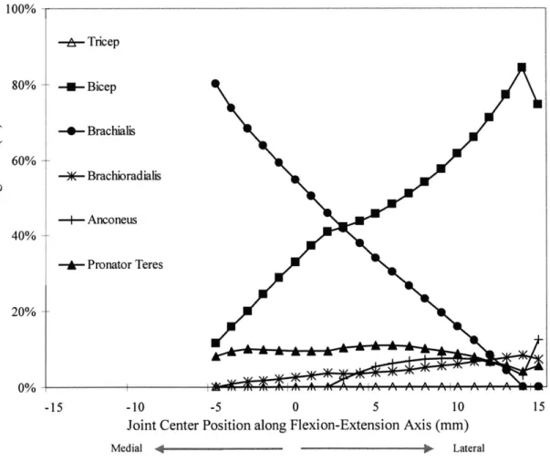
Optimization methods are widely used to predict in-vivo muscle forces in musculoskeletal joints. Moment equilibrium at the joint center (usually defined as the origin of the joint coordinate system) has been used as a constraint condition for optimization procedures and the joint reaction moments were assumed to be zero. This research project, through the use of a three-dimensional elbow model, investigated the effect of joint center location on muscle forces predicted using a nonlinear static optimization method. The results demonstrated that moving the joint center medially and laterally along the flexion-extension axis caused dramatic variations in the predicted muscle forces. For example, moving the joint center from a position 5 mm medial to 5
mm lateral of the geometric elbow center caused the predicted biceps force to vary from 12% to 46% and the brachialis force to vary from 80% to 34% of the total muscle loading. The joint reaction force reduced by 24% with this medial to lateral variation of the joint center location. This data revealed that the muscle forces predicted using optimization methods are sensitive to the joint center location due to the zero joint reaction moment assumption in the moment constraint condition. For accurate prediction of muscle load distributions using optimization methods, it is necessary to determine the true joint center location where the condition of a zero joint reaction moment is satisfied. Furthermore, improvements to the current optimization methodology were suggested. Incorporation of the 3D joint center location, as three unknown variables, into the optimization program was proposed, and this procedure was investigated for a pilot case incorporating one of the joint center components (y-axis variable) into the optimization. This thesis work indicates that all previously published data on muscle and joint loads predicted via optimization methods should be revisited since the joint reaction moment was eliminated in those works.
Thesis Supervisor: Guoan Li Title: Lecturer
Thesis Supervisor: Derek Rowell
Acknowledgements
I would like to thank my research advisor, Dr. Guoan Li, for the technical insight and valuable
advice he has so willingly bestowed upon me during my MIT career. In addition, many thanks are due to my academic advisor, Professor Derek Rowell, for his guidance throughout my master degree program. I am also very grateful for the generous funding I have received from the National Science Foundation (NSF) and the Orthopaedic Research and Education Foundation (OREF), both of which provided financial support crucial to the completion of this research project. There are also many other members of our research team, including Dr. Ephrat Most, Louis DeFrate, Jeremy Suggs, and Ramprasad Papannagari, to whom I extend my utmost thanks for all of their help over the course of this project. Finally, I would also like to thank my family for supporting me in my decision to leave the west coast and become a temporary Bostonian, my amazing boyfriend Grant who has made my graduate experience at MIT more worthwhile and fulfilling than I ever could have imagined, and my dear roommates and friends for providing endless encouragement and much needed comic relief during the past two years.
Table of Contents
LIST O F FIG U R ES ... 10
LIST O F TA BLES ... 13
CHAPTER 1: INTRODUCTION ... 15
1.1 H UMAN JOINT M ODELS... 15
1.2 N EW TON'S LAW S AND RIGID BODY M OTION ... 20
1.3 STATIC A NALYSIS OF A JOINT ... 21
1.4 INVERSE O PTIM IZATION M ETHODS ... 22
1.4.1 O bjective Functions ... 22
1.4.1.1 Physiological Relevance ... 22
1.4.1.2 Com m on Examples...23
1.4.1.3 Linear verses Nonlinear ... 25
1.4.2 Constraints ... 28
1.5 OTHER METHODS FOR MUSCLE LOAD DETERMINATION... 29
1.5.1 Force Reduction M ethod... 29
1.5.2 M uscle Scaling A pproach... 30
1.5.3 Cross-Sectional A rea and EM G Estim ations ... 30
CHAPTER 2: FOREARM ANATOMY AND RELEVANT TERMINOLOGY... 33
2.1 FOREARM BONES ... 33
2.2 M AJOR FOREARM M USCLES... 33
2.3 TERM INOLOGY ... 34
CHAPTER 3: MOTIVATION AND OBJECTIVE... 37
3.1 M OTIVATION ... 37
3.2 O BJECTIVE ... 38
CH A PTER 4: EX PER IM EN TA L SETU P ... 39
4.1 CADAVERIC SPECIM EN PREPARATION... 39
4.2 CADAVERIC EXPERIMENTAL TESTING... 40
4.2.1 Robotic Testing S stem ... 40
4.2.2 M icroscribe 3D X D igitizer ... 43
4.2.3 Cross-Sectional Com puterized Tom ography (CT) ... 43
4.3 THREE-D IM ENSIONAL M ODELING SOFTW ARE ... 44
CHAPTER 5: MODEL DEVELOPMENT ... 47
5.1 M USCLE LINES OF A CTIONS... 47
5.2 EQUILIBRIUM EQUATIONS... 47
5.3 O PTIM IZATION ... 51
5.3.1 O bjective Function and Constraints... 51
5.3.2 O ptim ization A lgorithm ... 51
CHAPTER 6: MODEL VALIDATION... 55
6.1 M OMENT A RM S... 55
6 .2 .1 E M G S etup ... 56
6.2.2 M aximum Voluntary Contraction... 56
6.2.3 Passive and Resisted Contraction Tests... 59
6.2.4 Data Processing... 59
6.2.5 Force Validation... 60
CHAPTER 7: RESULTS ... 65
7.1 JOINT CENTER VARIATION ALONG FLEXION-EXTENSION Axis... 65
7.1.1 M uscle Loading Ratios ... 65
7.1.2 Joint Reaction Force ... 69
7.1.3 Objective Function M inimum ... 71
7.2 JOINT CENTER VARIATION ALONG HUMERAL Axis ... 77
7.2.1 M uscle Loading Ratios ... 77
7.2.2 Joint Reaction Force ... 77
7.3 AUTOMATED JOINT CENTER OPTIMIZATION ... 81
7.3.1 Constant Force ... 81
7.3.2 Variable Axial M oment ... 85
7.3.3 Combined Loading... 89
CHAPTER 8: DISCUSSION ... ... 93
8.1 ZERO JOINT REACTION M OMENT ASSUMPTION ... 93
8.2 THE CASE FOR A M OVING JOINT CENTER LOCATION ... 94
8.3 VARIABLE JOINT CENTER LOCATION ... .... 95
8.3.1 Joint Center Variation along Flexion-Extension Axis ... 95
8.3.1.1 Effect of Location on Muscle and Joint Forces ... 95
8.3.1.2 Effect of Location on Objective Function Minima... 96
8.3.2 Joint Center Variation along Humeral Axis... 97
8.4 DIFFERENT OBJECTIVE FUNCTIONS...-.... 97
8.5 IMPROVEMENTS TO CURRENT INVERSE OPTIMIZATION M ETHODS ... 97
8.6 CLINICAL RELEVANCE ... ---.... ---... 99
CHAPTER 9: CONCLUSIONS AND FUTURE WORK ... 103
9.1 CONCLUSION...-... ---... 103
9.2 FUTURE W ORK... ... ---... 103
9.2.1 Advanced EM G Studies... 103
9.2.2 Rotation Center Validation ... 104
9.2.3 Experimental Studies ... .... 104
APPENDIX A: RIGID BODY M ECHANICS ... 107
A. 1 FORCE EQUILIBRIUM ... --... 108
A.2 M OMENT EQUILIBRIUM... 108
APPENDIX B: TWO-DIMENSIONAL STATIC EQUILIBRIUM EXAMPLES ... 111
APPENDIX C: EM G DATA... 116
C. 1 M AXIMUM VOLUNTARY CONTRACTION (M VC) TESTS... 116
C.1.1 Raw M VC Data... 116
C.2 ELECTROMYOGRAPHIC (EM G) DATA ... 120
C.2.1 Raw EM G Passive Flexion Test Data... 120
C.2.2 Raw EM G Resisted Flexion Test Data ... 122
C.3 N ORMALIZED EM G DATA... 124
C.4 M A TLAB CODES ... 127
C.4.1 M V C Value Determ ination... 127
C.4.2 Calculate RM S of Test Data... 129
C.4.3 N orm alize Data ... 131
APPENDIX D: OPTIMIZATION PROGRAM... 132
List of Figures
FIGURE 1-1. TIMELINE ILLUSTRATING SOME OF THE MAJOR RESEARCHER PAPERS PUBLISHED ON JOINT OPTIMIZATION M ETHODS IN THE PAST THREE DECADES. ... 16 FIGURE 2-1. NEUTRAL FOREARM FLEXION, AS VIEWED FROM THE SAGITTAL (FLEXION) PLANE. ... 35
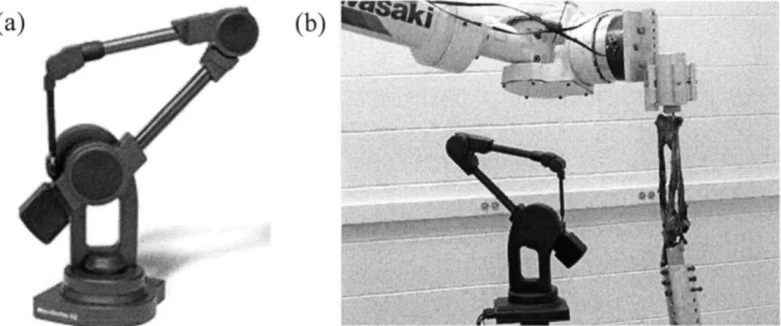
FIGURE 2-2. ILLUSTRATION OF PRONATED, NEUTRAL, AND SUPINATED FOREARM POSITIONS FOR A RIGHT FOREARM..35 FIGURE 4-1. PROTOCOL FOR EXPERIMENTAL SETUP AND MODEL DEVELOPMENT. ... 39 FIGURE 4-2. R OBOTIC TESTING SYSTEM ... 41 FIGURE 4-3. A FOREARM SPECIMEN, WITH SKIN REMOVED AND MUSCLES EXPOSED, IS RIGIDLY FIXED TO THE ROBOTIC SYSTEM (A). THE HUMERUS IS FIXED TO THE PEDESTAL ON THE BASE OF THE SYSTEM, AND THE RADIUS IS ATTACHED TO THE LOAD CELL. THE NEUTRAL PATH OF THE FOREARM IS OBTAINED (B) BY INCREMENTALLY FLEXING THE RADIUS WITH THE ROBOT OPERATING IN FORCE-CONTROL MODE. ... 41 FIGURE 4-4 (A) THE MICROSCRIBE 3DX DIGITIZER, MADE BY IMMERSION CORPORATION (SAN JOSE, CA), WAS USED TO TRACE THE MUSCLE INSERTIONS, ORIGINS, AND LINES OF ACTION, AND BONY GEOMETRY OF THE SPECIMEN. (B) IT WAS ALSO USED TO SET UP A COORDINATE SYSTEM FOR THE ROBOT/LOAD CELL WITH RESPECT TO THE JO IN T C EN T E R ... 4 5 FIGURE 4-5. (A) SINGLE CT SLICE OF FOREARM BONES WERE RECONSTRUCTED INTO A 3D SOLID IMAGE (B). ... 45
FIGURE 4-6. CALCULATED FLEXION-EXTENSION AXIS BY FITTING CIRCLES TO THE BOTTOM OF THE TROCHLEAR SULCUS, THE PERIPHERY OF THE CAPITULUM, AND THE MEDIAL FACET OF THE TROCHLEA. ... 45 FIGURE 5-1. FREE-BODY DIAGRAM OF FOREARM SYSTEM, INCLUDING MUSCLE FORCES, EXTERNAL LOADS, AND JOINT
REACTION FORCE AND M OM ENT...49 FIGURE 5-2. (A) COMPUTER-GENERATED 3D MODEL OF THE ELBOW JOINT AT 900 OF FLEXION AND (B) FREE-BODY
DIAGRAM OF ELBOW JOINT WHERE THE JOINT REACTION FORCE INCLUDES THE LIGAMENT TENSIONS AND ARTICULAR JOINT CONTACT FORCES...49 FIGURE 5-3. A SIMPLEX IS THE GEOMETRIC FIGURE COMPOSED OF N+1 VERTICES INTERCONNECTED BY LINE
SEGMENTS, WITH N DENOTING THE NUMBER OF VARIABLES USED IN THE OPTIMIZATION. A SIMPLEX IS (A) TRIANGULAR IN TWO DIMENSIONS (I.E. TWO VARIABLES IN THE OBJECTIVE FUNCTION) AND (B) TETRAHEDRAL IN THREE DIMENSIONS (I.E. THREE VARIABLES), AND SO FORTH. ... 53
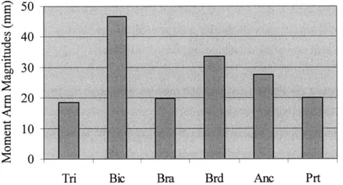
FIGURE 6-1. MOMENT ARM MAGNITUDES (GIVEN IN MM) CALCULATED FOR THE THREE-DIMENSIONAL CASE. ... 55
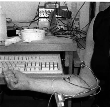
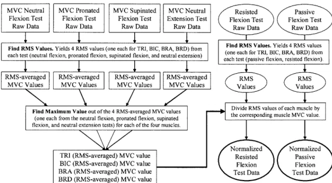
FIGURE 6-2. SUBJECT 2 PERFORMS PASSIVE CONTRACTION TEST IN THE SUPINATED FOREARM POSITION, WITH THE ELBOW HELD AT 900 OF STATIC FLEXION. ... 57 FIGURE 6-3. SCHEMATIC OF SUBJECT POSITIONING FOR PASSIVE AND RESISTED CONTRACTION EMG STUDIES...57 FIGURE 6-4. THIS FLOW CHART DEPICTS THE PROCESS BY WHICH THE RAW EMG DATA WAS PROCESSED AND
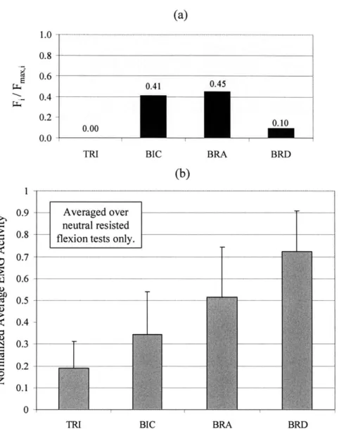
N O R M A L IZ E D ... 6 1 FIGURE 6-5. (A) RATIO OF PREDICTED MUSCLE FORCE MAGNITUDES (FI) TO MAXIMUM ISOMETRIC MUSCLE FORCE (Fm,1 ) VALUES (CALCULATED FROM cy*PCSA) FOR THE TRICEPS (TRI), BICEPS (BIC), BRACHIALIS (BRA),
BRACHIORADIALIS (BRD), ANCONEUS (ANC), AND PRONATOR TERES (PRT) AT 900 OF FLEXION, CALCULATED AT THE GEOMETRIC ELBOW JOINT CENTER (Y=0). (B) THE EMG ACTIVATION DATA, AVERAGED OVER DATA FROM FOUR NEUTRAL RESISTED FLEXION TESTS, IS SHOWN FOR THE TRI, BIC, BRA, AND BRD. EMG DATA WAS NOT COLLECTED FOR THE ANC OR PRT. THE EMG DATA SHOWS THAT THE BIC, BRA, AND BRD ARE ALL ACTIVATED AT 900 FLEXION, AS PREDICTED IN THE OPTIMIZATION (A). ... 63 FIGURE 7-1. THE JOINT CENTER WAS VARIED i 15 MM ALONG THE FLEXION-EXTENSION, OR Y, AXIS OF THE ELBOW. .67
FIGURE 7-2. THE PREDICTED MUSCLE LOADING RATIOS ARE PLOTTED AGAINST THEIR CORRESPONDING JOINT CENTER LOCATION ALONG THE FLEXION-EXTENSION AXIS (WITH A 50 N LOAD APPLIED AT THE DISTAL RADIUS AND NO
APPLIED AXIAL MOMENT). THE PREDICTED MUSCLE FORCES WERE HIGHLY SENSITIVE TO THE POSITION OF THE ELBO W JO IN T C EN TER . ... 67
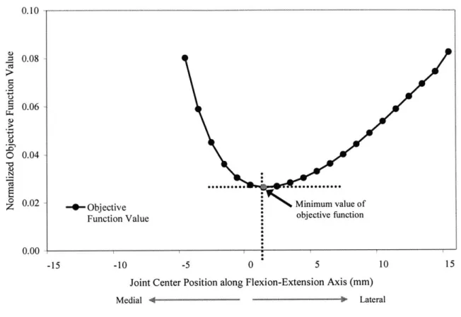
FIGURE 7-3. THE CHANGE IN THE JOINT REACTION FORCE (TOTAL MAGNITUDE AND HUMERAL, OR Z-AXIS, COMPONENT) IS PLOTTED AGAINST THE CORRESPONDING JOINT CENTER LOCATION ALONG THE FLEXION-EXTENSION AXIS (WITH A 50 N LOAD APPLIED AT THE DISTAL RADIUS AND NO APPLIED AXIAL MOMENT)...69 FIGURE 7-4. THE VALUE OF THE OBJECTIVE FUNCTION (NORMALIZED TO THE MAXIMUM POSSIBLE SUM OF THE CUBIC
MUSCLE STRESSES, 6a) WAS RECORDED AS THE JOINT CENTER LOCATION WAS TRANSLATED. THIS OBJECTIVE FUNCTION REACHED A MINIMUM VALUE AT 1 MM OF LATERAL TRANSLATION...73 FIGURE 7-5. VARIABLE LOADING CONDITIONS INCLUDING AN APPLIED MOMENT +5 N.M ABOUT THE X-AXIS AND AN
APPLIED LOAD OF -50N AT THE DISTAL RADIUS... 73 FIGURE 7-6. EXTERNAL MOMENTS RANGING FROM i 5 N.M WERE APPLIED TO THE X-AXIS OF THE FOREARM SYSTEM. THESE EXTERNAL LOADING CONDITIONS AFFECTED THE JOINT CENTER LOCATION AT WHICH THE OBJECTIVE FUNCTION REACHED A MINIMUM VALUE, AS DEPICTED FOR SELECTED LOADING CONDITIONS IN (A). THE MINIMA LOCATIONS FOR THE ENTIRE RANGE OF APPLIED MOMENTS (-5 TO 5 N.M) CAN BE SEEN IN (B), WHERE NEGATIVE AXIAL MOMENTS WERE SHOWN TO CAUSE A MEDIAL SHIFT AND POSITIVE AXIAL MOMENTS A LATERAL SHIFT IN THE OBJECTIVE FUNCTION MINIMA LOCATION...75 FIGURE 7-7. MOVEMENT OF THE JOINT CENTER PROXIMALLY AND DISTALLY ALONG THE HUMERAL (Z) AXIS
RESULTED IN VERY LITTLE CHANGE IN THE PREDICTED MUSCLE LOADING RATIOS...79 FIGURE 7-8. THIS FIGURE DEPICTS THE CHANGE IN THE JOINT REACTION FORCE (TOTAL MAGNITUDE AND HUMERAL, OR
Z-AXIS, COMPONENT) WITH PROXIMAL AND DISTAL VARIATION OF THE JOINT CENTER LOCATION ALONG THE HUMERAL (Z) AXIS (UNDER THE CONDITION OF A 50 N LOAD APPLIED AT THE DISTAL RADIUS AND NO APPLIED M O M EN T ) . ... 7 9
FIGURE 7-9. A CONSTANT LOAD WAS APPLIED AT THE DISTAL RADIUS (A) IN THE DIRECTION OF GRAVITY WITH A MAGNITUDE OF 50 N OR 100 N, AND (B) ACTING ALONG THE AXIS OF THE RADIUS WITH A MAGNITUDE OF 5 N OR
IO N ... 8 3
FIGURE 7-10. POSITION OF OPTIMIZED JOINT CENTER, AS CALCULATED AUTOMATICALLY FROM THE MODIFIED OPTIMIZATION PROGRAM, UNDER VARIOUS LOADS APPLIED AT THE DISTAL RADIUS...83 FIGURE 7-11. A MOMENT WAS APPLIED ABOUT THE X-AXIS OF THE JOINT SYSTEM FOR VALUES RANGING BETWEEN ± 5
N .M IN OVERALL M AGNITUDE. ... 85 FIGURE 7-12. EXTERNAL MOMENTS RANGING FROM + 5 N.M WERE APPLIED TO THE X-AXIS OF THE FOREARM SYSTEM, WITH NO ADDITIONAL APPLIED LOADS OTHER THAN THE WEIGHT OF THE FOREARM. THE "MANUAL" DATASET REPRESENTS OBJECTIVE FUNCTION MINIMA FOUND BY MANUALLY MOVING THE JOINT CENTER ALONG THE FLEXION-EXTENSION AXIS. THE "AUTO" DATASET REPRESENTS OBJECTIVE FUNCTION MINIMA DETERMINED AUTOMATICALLY FROM THE OPTIMIZATION...87 FIGURE 7-13. THE COMBINED LOADING CONDITIONS INCLUDE AN APPLIED AXIAL MOMENT (i 5 N.M) ABOUT THE
X-AXIS OF THE JOINT SYSTEM AND EITHER (A) AN APPLIED LOAD (50 N) AT THE DISTAL RADIUS ACTING IN THE DIRECTION OF GRAVITY OR (B) AN APPLIED LOAD (5 N) AT THE DISTAL RADIUS ACTING ALONG THE RADIAL AXIS.
... 8 9
FIGURE 7-14. EXTERNAL MOMENTS RANGING FROM + 5 N.M WERE APPLIED TO THE X-AXIS OF THE FOREARM SYSTEM, WITH A 50 N LOAD APPLIED AT THE DISTAL RADIUS IN THE DIRECTION OF GRAVITY. THE "MANUAL" DATASET REPRESENTS OBJECTIVE FUNCTION MINIMA FOUND BY MANUALLY MOVING THE JOINT CENTER ALONG THE FLEXION-EXTENSION AXIS. THE "AUTO" DATASET REPRESENTS OBJECTIVE FUNCTION MINIMA DETERMINED AUTOMATICALLY FROM THE OPTIMIZATION...91 FIGURE 7-15. EXTERNAL MOMENTS RANGING FROM ± 5 N.M WERE APPLIED TO THE X-AXIS OF THE FOREARM SYSTEM,
WITH A 5 N LOAD APPLIED AT THE DISTAL RADIUS ALONG THE AXIS OF THE RADIUS. THE "MANUAL" DATASET REPRESENTS OBJECTIVE FUNCTION MINIMA FOUND BY MANUALLY MOVING THE JOINT CENTER ALONG THE FLEXION-EXTENSION AXIS. THE "AUTO" DATASET REPRESENTS OBJECTIVE FUNCTION MINIMA DETERMINED AUTOMATICALLY FROM THE OPTIMIZATION...91
FIGURE 8-i. TWO-DIMENSIONAL SENSITIVITY ANALYSIS. THE JOINT CENTER WAS VARIED ALONG THE Z-AXIS (A) AND ALONG THE X-AXIS (B) TO DETERMINE HOW SENSITIVE THE PREDICTED MUSCLE AND JOINT FORCE WERE TO THE JO IN T CEN TER LOCA TION ... 10 1
FIGURE A-1. DESCRIPTION OF THE RIGID BODY SYSTEM OF N PARTICLES, EACH HAVING A UNIQUE MASS M,, WITH THE
ORIGIN OF THE COORDINATE SYSTEM CENTERED AT POINT 0...107
FIGURE B-1. TWO-DIMENSIONAL STATIC FLEXION EXAMPLE INVOLVING ONLY ONE MUSCLE FORCE, THE BRACHIALIS, AND TWO KNOWN EXTERNAL LOADS, THE WEIGHT OF THE ARM AND AN APPLIED LOAD AT THE DISTAL RADIUS. THE TWO COMPONENTS OF THE JOINT REACTION FORCE ARE ALSO UNKNOWN VALUES. ... III FIGURE B-2. THIS TWO-DIMENSIONAL STATIC FLEXION PROBLEM INVOLVES THREE MUSCLE FORCES (BRACHIALIS, BICEPS, AND BRACHIORADIALIS) AND TWO KNOWN EXTERNAL LOADS, THE WEIGHT OF THE ARM AND AN APPLIED LOAD AT THE DISTAL RADIUS. THE TWO COMPONENTS OF THE JOINT REACTION FORCE ARE ALSO UNKNOWN V A L U E S ... 114
FIGURE C-i. SUBJECT 1, MAXIMUM VOLUNTARY MUSCLE CONTRACTION TEST, LEFT ARM ... 116
FIGURE C-2. SUBJECT 1, MAXIMUM VOLUNTARY MUSCLE CONTRACTION TEST, RIGHT ARM ... 1 17 FIGURE C-3. SUBJECT 2, MAXIMUM VOLUNTARY MUSCLE CONTRACTION TEST, LEFT ARM ... 117
FIGURE C-4. SUBJECT 2, MAXIMUM VOLUNTARY MUSCLE CONTRACTION TEST, RIGHT ARM ... 1 18 FIGURE C-5. MAXIMUM OF THE RMS-AVERAGED VALUES (CALCULATED FROM FOUR FLEXION/EXTENSION TESTS) FOR THE BRD, TRI, BIC, AND BRA MUSCLES. THESE MAXIMUM RMS VALUES, ASSUMED TO BE THE MAXIMUM VOLUNTARY CONTRACTION (MVC) VALUE FOR EACH MUSCLE, WERE USED TO NORMALIZE THE TEST RESULTS (FOR THE CORRESPONDING SUBJECT/ARM COMBINATION) FROM THE PASSIVE AND RESISTED FLEXION TESTS. .119 FIGURE C-6. SUBJECT 1, PASSIVE FLEXION, LEFT ARM...120
FIGURE C-7. SUBJECT 1, PASSIVE FLEXION, RIGHT ARM ... 120
FIGURE C-8. SUBJECT 2, PASSIVE FLEXION, LEFT ARM...-121
FIGURE C-9. SUBJECT 2, PASSIVE FLEXION, RIGHT ARM ... 121
FIGURE C- 10. SUBJECT 1, RESISTED FLEXION, LEFT ARM ... 122
FIGURE C-11. SUBJECT 1, RESISTED FLEXION, RIGHT ARM ... 122
FIGURE C-12. SUBJECT 2, RESISTED FLEXION, LEFT ARM ... 123
FIGURE C-13. SUBJECT 2, RESISTED FLEXION, RIGHT ARM ... 123
FIGURE C-14. NORMALIZED DATA, SUBJECT 1, RESISTED FLEXION, LEFT ARM ... 124
FIGURE C-15. NORMALIZED DATA, SUBJECT 1, RESISTED FLEXION, RIGHT ARM...124
FIGURE C-16. NORMALIZED DATA, SUBJECT 2, RESISTED FLEXION, LEFT ARM ... 125
FIGURE C-17. NORMALIZED DATA, SUBJECT 2, RESISTED FLEXION, RIGHT ARM...125
FIGURE C-18. AVERAGE EMG ACTIVITY DURING FLEXION TESTS, AVERAGED OVER TWO SUBJECTS (FOUR ARMS) FOR THE PASSIVE AND RESISTED FLEXION TESTS...126
FIGURE C-19. AVERAGE EMG ACTIVITY FOR THE NEUTRAL FOREARM POSITION, AVERAGED OVER TWO SUBJECTS (FOUR ARMS), AND RECORDED WHILE PERFORMING THE RESISTED FLEXION TEST. ... 126
List of Tables
TABLE 2-1. MUSCLE PHYSIOLOGICAL CROSS-SECTIONAL AREAS (AN ET AL., 1981 [5])...34
TABLE 7-1. THE JOINT CENTER LOCATION, ESTIMATED MANUALLY AND FROM THE AUTOMATED PROGRAM, IS SHOWN FOR VARIOUS LOADING CONDITIONS...83
Chapter 1: Introduction
Engineers are the innovators and designers of complex machines and those machines are designed with specific engineering principles and analytical tools in mind. However, the musculoskeletal system of the human body is a complicated apparatus more involved and complex than any man-made machine one could possibly fathom. Consequently, in order to study the mechanical behavior of the human body, the bones, muscles, tendons, ligaments, and other structures must be reduced to a less complex system comprised of rigid links, actuators, and constraint elements. The elements of the system need to be clearly defined in mechanical terms, the external constraints on the system must also be identified, and the laws of motion can then be applied. Thus, the methods of rigid body mechanics can be applied to study the function of the human body only after the system is simplified and the model elements and their complexities are clearly defined.
1.1 Human Joint Models
The measurement of in-vivo muscle and joint reaction forces poses a distinct challenge in
biomedical engineering. To address this issue, numerous mathematical models have been
broadly adapted to calculate the response of muscles and musculoskeletal joints to external loads [1-41]. Various biomechanical models of human joints have been developed which constrained joint motion to a single plane, usually the sagittal or "flexion" plane [30, 34, 42-44], without evaluating the appropriateness or estimating the associated error of such an assumption. Many three-dimensional studies partially reduced the force distribution problem to the quasi-planar case by defining many or all of the joints as hinge, or one degree of freedom, joints [10, 12, 17,
29]. This hinge assumption caused two of the moment constraints to be removed before the
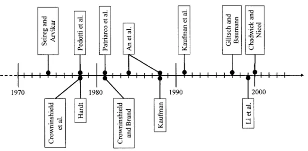
force computation was performed. Movement away from simple planar or quasi-planar models of human joints occurred in the early 90's with studies initiated by Kaufman et al. [21, 23] concerning the knee joint, followed by Glitsch and Baumann's [15] three-dimensional analysis of the lower extremity. In the paragraphs to follow, some of the major contributions to the field of joint modeling using inverse optimization methods are briefly summarized (Figure 1-1).
1970 ~C1 C~C1 1980 -od C -o -2 0 .0 .02 U U-C 1990 Cd -1 C ed 2000
Figure 1-1. Timeline illustrating some of the major researcher papers published on joint optimization methods in the past three decades.
Seireg and Arvikar (1973, 1975) were quite possibly the first investigators to develop a mathematical model that simulated the muscular action of the lower extremity without previously defining the active muscles and the forces they produce (or their respective force ratios) for the modeled activity (i.e. the model "chose" which muscles to activate and the force ratios to assign, not the investigator). They established a model of the lower extremity to evaluate muscle and joint reaction forces during specific static postures, including standing, leaning, and stooping [35], as well as during dynamic movements such as walking [36]. The model segmented the lower extremity into five rigid bodies: the pelvis, femur, tibia, fibula, and foot. A total of 29 muscles were considered in the analysis of these various movements. Since all activities were assumed to occur symmetrical with respect to the sagittal plane, the equilibrium of the pelvis was two-dimensional, thus requiring only three equilibrium equations (two force and one moment equation). The other three segments, however, were not restricted to sagittal plane movement, and thus were described by six equilibrium equations each (3 force and
3 moment equations), respectively. A total of 21 equilibrium equations, 29 unknown muscle
forces, as well as the unknown joint reaction forces and moments, made for an indeterminate problem. Using different linear optimization criteria, including minimization of muscular force and minimization of joint moment, and a simplex algorithm, the muscle and joint reaction forces for various activities were determined.
C
E 44
Pedotti et al. (1978) used a three link model of the lower extremity to investigate several different optimization criteria and the correlation of their force predictions with muscle EMG data [30]. Eleven muscles were used to simulate the gait motion, joint torques were computed from experimentally measured ground reaction forces and kinematic variables, and the model was restricted to an analysis of motion and forces in the sagittal plane. Analysis of four optimization criteria, all involving some form of total muscle force minimization, and comparison with recorded EGM data yielded the square of the (actual force)/(maximal force) for all muscles as the optimal performance criterion.
Hardt (1978) developed a model of the lower extremity, representing the hip and ankle as perfect ball joints and the knee as a simple hinge [17]. Thirty-one muscle forces were used in this 7 degree-of-freedom model. The linear minimization of muscle force criterion was used to solve for the unknown variables. The problem formulation involved 7 equality and no inequality constraints, leading to the prediction of only 7 active muscles for each time step analyzed. Hardt concluded that the linear penalty function employed was 'unnecessarily restrictive and leads to function definitions that are empirical in nature and may not have any physiological analog.' The proper solution to the optimization problem must therefore require more input regarding the physiology of the system and be viewed as an analogy to the physical system rather than purely a convenient mathematical methodology.
Crowninshield et al. (1978) developed an optimization model to investigate the mechanical environment of the human hip, i.e. the muscle and joint contact forces, during activities of daily living. The pelvis and lower extremity were modeled as four rigid segments: the pelvis, thigh, shank, and foot-shoe segment. These segments were assumed to be connected by smooth but loose ball-and-socket joints representing the hip, knee, and ankle, respectively. Twenty-seven muscles were identified as potential load-carrying structures at the hip during the daily activities simulated in the model. The knee and ankle were restricted to pure flexion-extensions motions, or sagittal plane motion, and modeled only for the sake of distributing the resultant forces at the hip. A linear objective function minimizing muscle stress was used to solve for the 27 muscles.
In 1981, Crowninshield and Brand defined what is currently the "gold standard" for objective functions used in joint optimization analyses, defining a new optimization criterion from the inversely-nonlinear relationship between muscle contraction force and endurance levels [12]. Crowninshield and Brand used this nonlinear optimization criterion to predict muscle forces in 1, the elbow during isometric contraction, and 2, the lower extremity (hip, knee, and ankle) during locomotion. For the elbow joint example, a simple planar model was employed requiring three of the elbow flexors (biceps, brachialis, and brachioradialis) to generate a fixed 10 N.m resultant moment. The lower extremity model was composed of 47 muscle elements, which were required to generate three orthogonal components of intersegmental moment at the hip and one component (flexion-extension) at the knee and ankle, respectively.
Hatze (1981) developed a mathematical model to simulate the motions of a 17-segment hominoid, or anthropomorphic mathematico-geometrical model of the segmented human body, under the influence of 46 muscles [18].
Based on a model of the lower extremity originally developed by Hardt [17], Patriarco et al.
(1981) studied the reliability of data acquisition and optimization procedures used to predicted
muscle forces during gait [29]. The lower extremity was modeled as a system of rigid links with the muscles regarded as torque generators. The seven measured joint torques, determined from kinematic studies, were used to loosely constrain the solution space when solving for the 31 muscles of the model. These torques corresponded to three degrees of freedom at the hip and ankle, and only one degree of freedom at the knee. Two optimization criteria were investigated,
including total muscle force and the mechanico-chemical energy output of the muscles.
An et al. (1984) sought to establish a new optimization approach to study the indeterminate joint problem [3]. The elbow joint was studied in quasi-2D in order to illustrate this approach. This model was formulated with nine muscles, which included the biceps brachii, brachialis, brachioradialis, pronator teres, supinator, triceps brachii, flexor carpi radialis, extensor carpi ulnaris, and extensor carpi radialis longus. Only two equilibrium equations, balancing the flexion-extension moment and the pronation-supination moment, were used to solve for the nine unknown muscle forces. An et al. presented another model of the elbow in a 1989 publication,
and this time assumed that the exerted torque at the elbow was primarily due to three muscles: the biceps brachii, brachialis, and brachioradialis [45]. The contributions of other forearm muscles were assumed insignificant, based on cross-sectional area or moment arm data, and were ignored. The muscle forces were predicted using a linear optimization method which sought to minimize muscle activation. The 3D force and moment equilibrium equations, as well as a modified tension-length relationship equation, constrained the solution.
K. Kaufman completed a Ph.D. dissertation (1988) on the development of a mathematical model of muscle and joint forces in the knee during isokinetic exercise [20]. Subsequently, Kaufman published a number of articles with colleagues in 1991 on the topic of joint modeling [21-23]. These articles outlined the formulation of a physiological model for predicting muscle forces using optimization to resolve the indeterminacy, and reported the predictions of knee joint forces during isokinetic exercise. The lower extremity was modeled as four rigid body segments: the pelvis, thigh, shank, and foot, but the foot was assumed to move with the shank as one integrated body. Muscular activation was chosen as the optimal criteria for force prediction.
Glitsch and Baumann (1997) set out to tackle the problem of three-dimensional internal load determination in the lower extremity [15]. Inverse dynamic and static optimization techniques, using a squared muscle stress criterion, were applied to a 3D model of lower limb containing 47 muscles. The load bearing capabilities of various joint types (hinge, spherical, and intermediate joints) were tested for the knee and ankle, resulting in the conclusion that even during seemingly planar movements like walking, significant three-dimensional intersegmental moments were produced. This study claimed up to a 60% underestimation of loads predicted using 2D methods, and addressed the inappropriateness of modeling the knee and ankle as hinges.
Li et al. (1999) used an inverse dynamic optimization model to predict antagonistic muscle and joint reaction forces in the knee during isokinetic flexion and extension [26]. A total of ten muscles were used to simulate knee joint motion, which included flexion/extension, varus/valgus, and internal/external rotations. Four optimization criteria were implemented and all four predicted antagonistic muscle contraction. The results suggested that the kinematic
information involved in the inverse dynamic optimization was more crucial to the prediction of the antagonistic muscle forces than the selected optimization criterion.
Chadwick and Nicol (2000) developed a 3D model of the elbow and wrist joints comprised of 15 muscle, 3 ligament, and 4 joint forces [9]. External moments were experimentally determined with a newly developed strain gauge transducer, and these moments were assumed to be balanced by the internally generated joint moment, thereby yielding an indeterminate set of equations. A dual-stage linear programming approach was implemented to first minimize the sum of the muscle stresses and then minimize the sum of the joint and ligament forces. Four different grip positions were studied and the corresponding joint forces were determined.
1.2 Newton's Laws and Rigid Body Motion
Estimating the internal forces in the musculoskeletal system in response to any external loads requires the use of engineering mechanics, as governed by the laws of motion. The laws of motion for rigid bodies are derived from Newton's 1st, 2 nd, and 3 rd laws.
Newton's 1st Law: When the sum of the forces acting on a particle is zero, its velocity is
constant. In particular, if the particle is initially stationary, it will remain stationary. Newton's 2nd Law: When the sum of the forces acting on a particle is not zero, the sum of
the forces is equal to the rate of change of the linear momentum of the particle. If the mass is constant, the sum of the forces is equal to the product of the mass of the particle and its acceleration.
Newton's 3rd Law: The forces exerted by two particles on each other are equal in
magnitude and opposite in direction [46].
The derivation of the rigid body motion equations can be found in Appendix A. The second law is probably most recognized in the form of the rigid body equilibrium equation,
ZP = ma, (1-1)
where m is the mass of the body and a is its linear acceleration. This is probably the most utilized equation in the study of motion analysis, and is applicable when the mass is constant. Additionally, under any planar motion the total moment about the center of mass is denoted by
where I is the mass moment of inertia about the center of mass and a is the angular acceleration. Additionally, if the rigid body rotates about a fixed axis 0, the sum of the moments about 0 relates to the angular acceleration and moment of inertia about 0 by
EMO = I . (1-3)
However, in the absence of motion, the equations reduce to the simplified form:
EP =0
(1-4)
EM= 0
These two vector equations represent 4 scalar equations for the two-dimensional case and 6 scalar equations when considering the three-dimensional case. A simple example for the two-dimensional planar case can be seen in Appendix B.
1.3 Static Analysis of a Joint
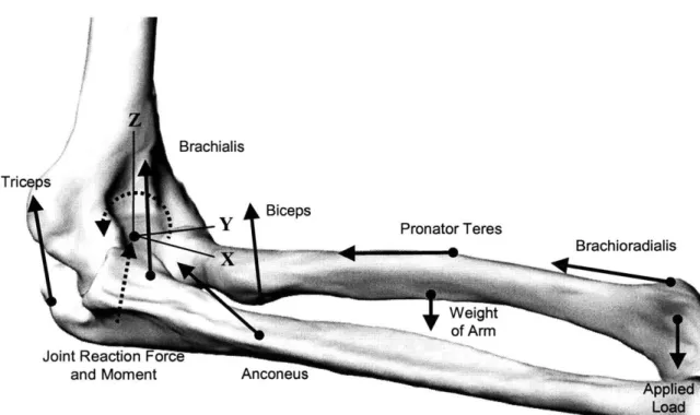
At any flexion angle or position of the joint, the external force system (including applied moments and forces, and the weight of the limb) was balanced by the internal force system (including muscle forces, joint reaction forces and moments). The joint reaction force, illustrated in Figure 5-2b for the elbow joint, is comprised of the remaining internal forces (excluding muscle forces) which may include joint articular contact, ligamentous, capsular, and passive soft tissue deformation forces. Utilizing the simplified laws of motion for static analyses (Equation 1-4) and a free-body diagram of the joint (see Figure 5-1 for the elbow joint), the following force and moment equilibrium equations were obtained for the static joint analysis:
[N
(a) Lf f M , ± fJoint _ int
i=1
N (1-5)
(b) ~fM(Fx)p7 Joint 1 1int(15 (b) X ji x +
XI"'-where fm is the magnitude and Z, is the direction of the i-th muscle force; T, is the vector
pointing from the joint center to the insertion centroid of i-th muscle; P "'"' and MO"' are the
joint reaction forces and moments; and Pint and R"' are the intersegmental forces and moments
moment equation for each of the three dimensions) contain N muscle force magnitudes, 3 components of the joint reaction force, and 3 components of the joint reaction moment. This represents a statically indeterminate system. Thus, human joints are very complex indeterminate systems whose muscle and joint forces cannot be solved for directly and must instead be predicted using inverse optimization methods.
1.4 Inverse Optimization Methods
Optimization is a mathematical method by which an indeterminate system of equations is iteratively solved by maximizing or minimizing an objective function, often subjected to various constraints [3, 5, 9, 15, 23, 26, 30, 35, 36]. Thus, an optimization problem can be thought of as containing three major components:
1. An objective function which is either maximized or minimized.
2. A set of unknowns or variables which affect the value of the objective function.
3. A set of constraints that allow the unknowns to take on certain values but exclude
others.
A human musculoskeletal joint (e.g., elbow, knee, etc.) is an indeterminate biomechanical
system in nature. The number of unknown forces generated by each muscle, as well as the unknown joint reaction force and moment components, outnumber the equilibrium equations of the joint system [23]. A unique solution for these forces cannot be obtained directly and must instead be estimated through the use of optimization techniques.
1.4.1 Objective Functions
Optimization, as stated above, necessitates the definition of an objective or cost function for the purpose of mathematically finding its minima or maxima. This objective function is comprised of unknowns that are of interest to the problem at hand and, in the case of human joint function, this usually constitutes variables physiologic in nature.
1.4.1.1 Physiological Relevance
Studying energy expenditure and its minimization has long dominated research in the scientific
and engineering disciplines. Muscular activity, not unlike a mechanical system, is also
associated with energy expenditure in such forms as mechanical, chemical, and heat. For over a century, researchers have hypothesized that the body functions in such a way as to minimize the
amount of energy spent [47, 48]. Weber and Weber (1836) proposed that humans walk in a manner that requires the smallest amount of energy expenditure. Thus, the idea that the body moves in an efficient or optimal manner was popular long before optimization approaches were first utilized to estimate in-vivo muscle loads in the field of biomechanics. The introduction of optimization to study such physiologic parameters as muscle loads led to the investigation of potentially "physiologically relevant" objective functions which would ultimately minimize energy expenditure. Fittingly, MacConaill (1967) suggested that "no more total muscle force is used than is both necessary and sufficient for the task to be performed, whether this be one of supporting some weight or carrying out a movement, resistance to which may vary from zero upwards [49]."
Many of the objective functions used in the joint modeling literature were chosen because they made the most sense physiologically. The human body, just like any mechanical system, wants to maximize its performance while minimizing the forces or stresses on its components. Therefore, minimizing force, stress, and energy were deemed to be excellent objective functions for such an optimization since it would be tough on the body if it used more energy than it needed, given the number of cycles its joints are subjected to on a daily basis.
1.4.1.2 Common Examples
All optimization procedures operate under the assumption that the body selects muscles for a
certain activity according to some criterion, usually seeking to minimize some "objective function" or "cost function", with muscle activity predictions often varying greatly depending on the choice of criteria. Some popular objective functions are discussed below and include the minimization of such parameters as the total muscular force, squared muscular force, muscle stress, squared or cubic muscle stress, ligament force, contact force, or instantaneous muscle power [43].
e Muscle Stress
Crowninshield and Brand [12] proposed the minimization of maximum stress in the active
muscles as a physiological criterion to minimize muscle fatigue. More specifically, they
recommended minimization of the total cubic muscle stress, and this particular objective function has been applied by many authors in the study of knee muscle forces during various
in-vivo functional activities, among other applications. Glitsch and Baumann used a squared muscle stress criterion for the determination of three-dimensional internal loads in the lower extremity [15]. The persistence of muscle stress as a popular cost function is illustrated by its recent appearance in a 2003 article by Oizumi et al. [28], in which the sum of the squared muscle force divided by the muscle cross-sectional area was used to perform a numerical analysis of cooperative abduction muscle forces in a human glenohumeral joint.
9 Muscle Force
The minimization of the total muscle force criterion, implemented by MacConnaill (1967) in a study of knee joint equilibrium forces, assumed that the summation of the magnitude of individual muscle forces should be minimized in order to ensure dynamic equilibrium of the joint [49]. Seireg and Arvikar (1975) used a criterion which represented a weighted combination of two objectives: 1, minimizing the total sum of all muscle forces, and 2, minimizing the forces in the joint ligaments assumed to carry the unbalanced joint moments. The criterion consisted of the sum of the muscle forces plus four times the sum of the moments at all the joints [36].
Three decades after the introduction of the muscle force criterion my MacConnaill [49], Happee (1994) implemented a weighted sum of the squared muscle forces criterion, using inverse dynamic optimization to study goal directed movements [50].
Total muscle force and total squared muscle force [30, 49] both minimize the overall effort (muscular force) required for an activity. The squared force, however, has been shown to greatly penalize large individual muscle forces [30].
e Joint Reaction Force or Moment
In a 1973 study modeling the lower extremity, Seireg and Arvikar tested a number of possible optimization criteria, one being minimization of the sum of the three vertical reactions at the ankle, knee, and hip joints, respectively [35]. The joint moment criterion minimizes the total moment generated by all muscles with respect to the joint center, as used by Seireg and Arvikar
[36] for the center of the knee joint. e Muscular Activation
The muscular activation criterion minimizes the upper bound value of the overall activation of all muscles. Activation refers to both the number of active units (recruitment) and their degree of activity (firing frequency) [45]. Kaufman et al. (1991) put forth muscular activation as the optimal cost function for determining loads at the knee joint [21, 23]. This is similar to the criteria minimizing muscular stress (or maximizing endurance time) outlined by Crowninshield and Brand [12], which sought to minimize muscular fatigue.
* Mechanico-chemical energy output [29]
Hardt (1978) hypothesized that forces are distributed among muscles during activities, such as
walking, by minimizing energy consumption [51]. Calculation of this muscle energy
consumption was achieved through the development of a thermodynamic model relating input chemical energy to output mechanical power. This thermodynamic model took into account the chemico-mechanical dynamics of the energy transfers occurring in muscles. However, it was specified that this model, and thus this objective function, was only valid for low frequency activities in the same range as walking.
1.4.1.3 Linear verses Nonlinear
In order to predict co-activation between synergistic muscles, and achieve more accurate muscle force predictions in general, researchers have migrated away from linear cost functions. Linear optimization techniques have seemingly been used more out of mathematical convenience than to achieve physiologic accuracy in muscle load predictions. The primary characteristic of linear objective functions is to minimize the number of loaded structures whereas nonlinear objective functions tend to distribute the load among all the structures involved.
* Linear
One very attractive feature of the linear objective function, which may explain the persistence of linear objective functions in the joint modeling literature, is that it can be minimized, and the unknowns solved for, via a linear programming method. This is much easier to implement and code than a nonlinear scheme, giving rise to its popularity. An example of one such popular and easy to use linear objective function is the minimization of the total muscle forces [6, 11, 44]:
N
As stated previously, linear objective functions often tend to minimize the number of loaded structures. This means that when using a linear objective function to solve for muscle forces, it will generally give the result that only one muscle force is active at a time (setting other muscle forces to zero) to achieve its minimum value. This is contrary to experimental results, such as electromyographic (EMG) analyses, which show generally more than one muscle active across a joint during a given activity. To try to combat this drawback of the linear objective function, additional constraints in the form of muscle force or stress limitations have been imposed to better define the solution space.
Barbenel (1972) challenged the principle of total muscle force while studying the temporomandibular joint [7]. Using linear programming to minimize the total muscular force, only the masseter muscle was predicted to be active during biting. EMG analysis and muscle palpation during biting showed, at minimum, the masseter, internal pterygoid, and temporal muscles were active. Likewise, Yeo et al. (1976) attempted to use the total muscle force objective function to predict muscle forces during elbow flexion [44]. The brachioradialis was predicted to be the primary flexor, with the biceps and brachialis only being activated if the brachioradialis was stimulated to saturation. EMG data, conducted by Basmajian and Latif
(1957) contradicted such predictions [52], leading Yeo et al. to conclude that this objective
function was insufficient for determining in-vivo muscle loads [44].
Seireg and Arvikar (1973, 1975) applied linear optimization criteria to a model of quasi-static locomotion and predicted very few simultaneously active muscles and unrealistically low joint contact forces during gait [35, 36]. This is an inherent problem in linear optimization and is related to the fact that the solution usually resides in the corner of the solution space, thereby predicting very few muscles to be active.
Hardt (1978) found that the number of predicted muscles for an activity simulated using linear optimization was limited to the total number of constraints placed on the optimization [17]. This inadequacy in force predictions clearly has no physiological significance and is purely a limitation of the optimization procedure itself.
An et al. (1984) experimented with different objective functions for calculating muscle forces across the elbow joint [3]. The summation of the muscle force and the summation of the muscle stress, both linear objective functions, predicted only one muscle to carry force in each solution. When minimizing the sum of the forces, the muscle with the largest moment arm was selected in the solution. Contrastingly, when minimizing the muscle stresses as the linear criterion, the muscle with the largest physiological cross-sectional area was selected in the solution. Practically speaking, this means that the optimization algorithm recruited the muscle with the largest PCSA until it reached its maximum force, and then, if necessary, it recruited the muscle with the next largest PCSA.
Advances in linear optimization have been made to try to address this problem. Efforts have been made to use weighted, linear combinations of muscle and joint forces as new criteria, but agreement of the force predictions with EMG experiments has not been desirable [3]. Bean et al.
(1988) developed a double linear programming approach that simultaneously minimized two
different objective functions, one being the minimization of muscle intensity (stress) and the other minimizing the sum of the muscle forces [53]. Through this method, it was demonstrated that co-activation predictions are possible with linear programming; however, results were not compared with EMG data. Kaufman et al. (1991) avoided the typical muscle and joint force criteria and used muscle activation as a cost function to predict muscle forces in the knee joint
[23]. He concluded that properly constrained linear programming methods do not limit the
number of active muscles and allow for uniform recruitment of the active muscles.
e Nonlinear
Unlike linear objective functions, nonlinear cost functions tend to distribute the load among all
involved structures. In an effort to find a physiologically relevant objective function,
Gracovetsky et al. (1977) minimized the sum of the squared shear forces in vertebral discs under the assumption that this parameter was related to human performance and injury prevention [54]. Likewise, Pedotti et al. (1978) used a number of objective functions, including the total squared muscle stress, to solve for muscle forces in walking under the hypothesis that such objective functions minimized energy during locomotive tasks. In 1981, Crowninshield and Brand [12] incorporated a physiological argument, supported by a quantitative force-endurance relationship
[55], into a nonlinear objective function by proposing the following objective function (Equation 1-7) to minimize the sum of the muscle stresses, raised to nth power:
n
Minimize J= N
L.
(1-7)This objective function was based on the idea that muscle fatigue must be related to the physiologic stress in the muscle. It can be solved by linear, quadratic, or nonlinear programming
depending on choice of n. Crowninshield and Brand [12] recommended the choice of n = 3 since
the amount of time a muscle can sustain activity is inversely proportional to the muscle stress raised to the power of three [55]. This seems to make physiological sense due to the fact that relatively high muscle stress can only be sustained for short periods of time whereas lower muscle stresses can be sustained for much longer time periods. Thus, in an objective or cost function sense, high muscle stresses are costly and should be avoided.
1.4.2 Constraints
Optimization is a mathematical method of minimizing an objective function subjected to various constraints. The typical constraints used to limit the solutions obtained from a joint optimization problem can be seen below:
N
(a) Lf M +PJoi"t =Pint N
(b) f x ,) - .
(-(c) 0 fM" o-A - A
The first constraint (a) is easily recognized as the force equilibrium equation, requiring that the muscle forces, joint reaction forces, and intersegmental forces must balance each other in all three directions. The moment equilibrium about the selected joint center (b) must also be satisfied [21, 23, 25, 26]. This constraint requires that the moments about the joint center, induced internally by muscle forces and externally by applied loads, sum to zero in all three directions, with the assumption of no joint reaction moment [15, 25, 26, 32]. The third constraint (c) requires that the muscle forces be positive, or non-compressive, since
physiologically-speaking muscles can only exert a tensile force. Additionally, the force values were further constrained with a condition limiting the upper bound on muscle force to a maximum isometric force value, obtained by multiplying the individual muscle physiological cross-sectional area (A1) by a constant maximum physiological muscle stress value (c-) [9, 10, 23, 30, 45, 56].
Historically, additional constraints to try to redistribute the loads between functionally similar muscles have also been imposed. Similar to the constraint described above, Patriarco et al.
(1981) tried to encourage simultaneous muscle activations in a lower extremity model by
imposing stress limits on muscles which forced synergistic action if a muscle exceeded its stress limit [29]. These bounds, however, were defined by the velocity and length dependence of stress limits, as determined from Hill's (1953) muscle model [57]. A second technique employed by Patriarco et al. (1981) to encourage synergistic action during gait constrained similar muscles to share load in proportion to their cross-sectional areas [29]. This was based on the physiological assumption that anatomically distinct muscles with very similar moment arms are functionally interchangeable during gait and, although unproven, this assumption was suggested after observing the close correlation of their EMG data.
1.5 Other Methods for Muscle Load Determination
There are many methods that have been developed to solve for in-vivo muscle loads without the use of a mathematical system of equations, or by reducing an initially indeterminate system to one that is determinate through simplification.
1.5.1 Force Reduction Method
If optimization methods are not employed to solve the indeterminate system which describes a
complex joint, researchers tend to simplify the system to include only as many unknowns as they have equations [58-60]. Muscles are either grouped together, deemed insignificant, or altogether ignored. When considering a single joint, if the joint reaction force is considered an unknown variable (with 3 components for the 3D case), then only 3 additional unknown variables can be determined from the equilibrium equations (Equation 1-5). This corresponds to 3 muscle force magnitudes if the muscle lines of action are known. The simplest means of reducing the number of muscles is to set enough individual forces to zero until the number of unknowns matches the number of equations. This can include identifying and using only the most dominant muscles for
that activity, or grouping multiple muscles which insert at a single point (e.g. the quadriceps insertion on the patella) together as one resultant force. Muscles are often combined into groups on the basis of synchronous EMG activity for a certain action [61]. Also, muscles become good contenders for being set to zero if they lack significant EMG activity for the specified action. This force reduction method of eliminating/combining variables to reduce the number of unknown muscle forces around a joint in a distribution problem results in the loss of information about the function of individual muscles [37, 60], thereby making it a highly undesirable approach.
1.5.2 Muscle Scaling Approach
Another alternative method for solving the indeterminate system is to eliminate the indeterminacy by introducing additional equations based on the equal stress hypothesis for groups of co-operating muscles. This hypothesis states that, in a strenuous situation, muscles which are co-operating in a group (such as the flexors of the forearm) are likely to have their fibers similarly stressed as their maximum strength is approached [2]. Thus, the forces, Fi, of the different muscles contributing to the activity being modeled can be estimated by assuming each
muscle acts at the same stress level, denoted by (, where a = Fi /Ai for each individual muscle i
with physiological cross-sectional area Ai. Using this method, without the use of optimization, Amis et al.[2] predicted the loading of individual flexor muscles at equilibrium from a known
external force.
1.5.3 Cross-Sectional Area and EMG Estimations
It is also common to apportion muscle loading in accordance with muscular size and activity. Muscle force ratios have been defined directly from EMG data in combination with physiological cross-sectional areas [31, 62, 63], estimated solely from a ratio of physiological cross-sectional areas [39], or arbitrarily assigned specific ratios or magnitudes [64-66]. Poppen and Walker (1978) performed an analysis to determine the forces in the glenohumeral joint during isometric abduction. The main assumption in their analysis was that the force in a muscle
was proportional to its area times the integrated electromyographic signal [31]. Likewise,
Johnson et al. (2000), in an attempt to simulate elbow joint motion with a load controlled testing apparatus, used a muscle loading ratio criterion determined directly from the product of the relative muscle EMG activity and the muscle physiological cross-sectional area data [62].
Wuelker et al. (1995) used a constant force ratio, determined from the ratio of muscle
cross-sectional areas, to define forces in the shoulder musculature [39]. In an effort to study
unconstrained glenohumeral joint motion, Debski et al. (1995) applied the same force to each tendon of the rotator cuff [66] during experiments performed in a dynamic shoulder testing apparatus.
Chapter 2: Forearm Anatomy and Relevant Terminology 2.1 Forearm Bones
The human arm is composed of three bones: the humerus, radius, and ulna. The distal end of the humerus articulates with the proximal ends of the forearm bones, the radius and ulna, constituting the elbow joint. Two epicondyles project from the lateral and medial sides of the
distal humerus. The articulating surface of the humerus extends slightly lower than the
epicondyles and includes the capitulum, a knob-like structure on the lateral aspect that articulates with the radial head, and the trochlea, a spool or pulley-shaped boney structure on the medial aspect that articulates with the semiulnar notch of the ulna.
2.2 Major Forearm Muscles
Six major flexors and extensors of the forearm [5, 32, 67] were identified prior to the formulation
of the elbow joint model. The triceps brachii (TRI) is a large spindle-shaped muscle which lies on the posterior side of the arm, with an insertion on the olecranon process of the ulna. It is composed of three components: the long head, medial head, and lateral head, which have three separate origin sites on the inferior portion of the glenoid (on the scapula), the entire posterior surface of the humerus below the radial groove, and the posterior surface of the upper humerus (above the radial groove), respectively. The main functions of the triceps brachii include extension of the forearm and adduction of the arm (shoulder compression). The biceps brachii (BIC) is a powerful muscle which lies anteriorly in the arm. It consists of two heads: the long head, which wraps around the head of the humerus, and the short head. The biceps brachii scapula and coracoid process of the scapula, respectively. Its main functions include flexion and supination of the forearm. The brachialis (BRA) is a flattened, spindle-shaped muscle which lies posterior to the biceps brachii. It inserts on the front of the coronoid process of the ulna, and originated on the lower frontal portion of the humerus. The primary function of the brachialis is to flex the forearm. The brachioradialis (BRD) is an elongated, spindle-shaped muscle which runs along the outer side of the radius. It inserts on the lateral port of the radius above the styloid process, and originates on the lateral supracondylar ridge of the humerus. The brachioradialis functions mainly as a flexor of the forearm, and is also utilized for supination during forearm extension. The anconeus (ANC) is a triangular-shaped muscle which wraps across the posterior
portion of the radial head. It inserts on the outer margin of the olecranon process of the ulna and originates on the posterior surface of the external condyle of the humerus. The anconeus is actively involved in extension of the forearm. The pronator teres (PRT) is a small rounded muscle lying on the frontal side of the forearm. The insertion is near the middle of the radius on the outer side of the shaft, and its origin lies on the medial epicondyle of the humerus. The primary function of the pronator teres is to pronate the forearm [68, 69].
2.3 Terminology
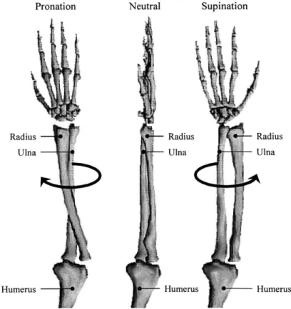
Flexion angle refers to the angle made by the long axis of the humerus and the axis of the forearm, as measured in the sagittal or flexion plane (Figure 2-1). Supination refers to the rotation of the radius about the ulna, such that the palm faces forward or upward and the radius lies parallel to the ulna. Pronation refers to the opposite direction of rotation of the radius about the ulna such that the palm faces backwards or downwards. The neutral forearm position, often termed the neutral wrist position, refers to a position of the radius with respect to the ulna that is halfway between fully pronated and fully supinated rotation, or a mid-pronation/supination position (Figure 2-2).
The physiological cross-sectional area (PCSA) of a muscle is obtained by dividing the muscle volume by its true fiber length, and is defined in units of length squared. "The rationale of this definition is simply that the cross-sectional area of a muscle is proportional to the number of its fibers and the individual muscle fiber is the basic element which generates the active tension
[23]." PCSA values of the primary forearm muscle flexors and extensors are defined in Table
2-1 and were obtained from data complied by An et al. [5].
Table 2-1. Muscle physiological cross-sectional areas (An et al., 1981 [5])
Muscle Group Muscle Abbreviation PCSA (cm2) Total PCSA (cm2
)
Long Head 6.7
Triceps Brachii Medial Head TRI 6.1 18.8
Lateral Head 6.0
Long Head 2.5 4.6
Biceps Brachii BIC4.
Short Head 2.1
Brachialis BRA 7.0 7.0
Brachioradialis BRD 1.5 1.5
Anconeus ANC 2.5 2.5
-60*
Figure 2-1. Neutral forearm flexion, as viewed from the sagittal (flexion) plane.
Pronation Neutral Supination
Radius -Radius Radius
Ulna Ulna Ulna
Humerus Humerus Humerus