HAL Id: hal-00023223
https://hal.archives-ouvertes.fr/hal-00023223
Submitted on 21 Apr 2006
HAL is a multi-disciplinary open access
archive for the deposit and dissemination of
sci-entific research documents, whether they are
pub-lished or not. The documents may come from
teaching and research institutions in France or
abroad, or from public or private research centers.
L’archive ouverte pluridisciplinaire HAL, est
destinée au dépôt et à la diffusion de documents
scientifiques de niveau recherche, publiés ou non,
émanant des établissements d’enseignement et de
recherche français ou étrangers, des laboratoires
publics ou privés.
High Accuracy 65nm OPC Verification: Full Process
Window Model vs. Critical Failure ORC
Amandine Borjon, Jerome Belledent, Shumay D. Shang, Olivier Toublan,
Corinne Miramond, Kyle Patterson, Kevin Lucas, Christophe Couderc, Yves
Rody, Frank Sundermann, et al.
To cite this version:
Amandine Borjon, Jerome Belledent, Shumay D. Shang, Olivier Toublan, Corinne Miramond, et al..
High Accuracy 65nm OPC Verification: Full Process Window Model vs. Critical Failure ORC. 2005,
pp.1750-1761. �hal-00023223�
High Accuracy 65nm OPC Verification: Full Process Window Model
vs. Critical Failure ORC
Amandine Borjon1, Jérôme Belledent1, Shumay D. Shang2, Olivier Toublan2, Corinne Miramond3, Kyle Patterson4, Kevin Lucas4, Christophe Couderc1, Yves Rody1, Frank Sundermann3, Jean-Christophe Urbani3, Stanislas Baron3, Yorick Trouiller5, Patrick Schiavone5.
1 Philips Semiconductors 850 rue J.Monnet 38926 Crolles, France, 2
Mentor Graphics Corporation, 1001 Ridder Park Drive, San Jose, CA 95131,
3 STMicroelectronics 850 rue J. Monnet 38926 Crolles, France, 4 Freescale Semiconductor 850 rue J. Monnet 38926 Crolles, France, 5 LETI-CEA- 17 rue des Martyrs 38054 Grenoble, France,
ABSTRACT
It is becoming more and more difficult to ensure robust patterning after OPC due to the continuous reduction of layout dimensions and diminishing process windows associated with each successive lithographic generation. Lithographers must guarantee high imaging fidelity throughout the entire range of normal process variations. The techniques of Mask Rule Checking (MRC) and Optical Rule Checking (ORC) have become indispensable tools for ensuring that OPC delivers robust patterning. However the first method relies on geometrical checks and the second one is based on a model built at best process conditions. Thus those techniques do not have the ability to address all potential printing errors throughout the process window (PW). To address this issue, a technique known as Critical Failure ORC (CFORC) was introduced that uses optical parameters from aerial image simulations. In CFORC, a numerical model is used to correlate these optical parameters with experimental data taken throughout the process window to predict printing failures. This method has proven its efficiency for detecting potential printing issues through the entire process window [1].
However this analytical method is based on optical parameters extracted via an optical model built at single process conditions. It is reasonable to expect that a verification method involving optical models built from several points throughout PW would provide more accurate predictions of printing failures for complex features. To verify this approach, compact optical models similar to those used for standard OPC were built and calibrated with experimental data measured at the PW limits. This model is then applied to various test patterns to predict potential printing errors.
In this paper, a comparison between these two approaches is presented for the poly layer at 65 nm node patterning. Examples of specific failure predictions obtained separately with the two techniques are compared with experimental results. The details of implementing these two techniques on full product layouts are also included in this study.
Keywords: OPC, Critical Failure ORC, process window, ORC, MRC, failure prediction.
1.
Introduction:
With current lithographic technology the need for post-OPC patterning verification has become critical. Indeed imaging at low-k1 leads to an improved sensitivity of patterns to process variations. To prevent hard failures from happening Mask Rule Checking (MRC) and Optical Rule Checking (ORC) have been introduced. But as MRC technique is based on geometrical rule verifications and ORC techniques relies on a check at best process conditions, the consequence of a small change in dose or focus on CD line cannot be fully assessed by these techniques.
To address this issue post-OPC verification techniques calibrated with process window data have recently been built. This study consists of a comparison between the Critical Failure ORC (CFORC) technique and a full Process Window model (full PW model). The CFORC technique uses a numerical model correlating optical parameters to PW experimental data so that optical parameters extracted at any polygon edge give information on its printing behaviour. The full PW model consists of compact optical models generated at several defocus conditions coupled with a global variable threshold resist
model calibrated across PW. Printing failures are detected by simulating resist printing through the entire PW.
The objective of this study is to compare these two techniques on their model building flow, their cycle-time on real layout and their error predictions. For doing so the comparison will be held on the poly layer at the 65 nm node. Its printability characteristics will be explored and modelled through a depth of focus of ±0.100µm and a dose variation of ±5%.
2.
Models building and models accuracy:
In this section we will describe the principles of each technique through its model flow and we will also check the accuracy of the models generated for the study.
2.1 CFORC model
2.1.1 CFORC model calibration
CFORC is a technique which requires a different model flow from the OPC model flow (fig
2.1) (refer to previous papers [1] [2] for the entire methodology). Indeed at the first step of the
calibration flow extra calibration test-patterns have to be built for the calibration. They consist of a matrix of symmetrical 1D or 2D patterns in which the design changes slightly from one pattern to another so that under dose or/and focus variations some of these test-structures encounter printing failures. They are then implemented on a mask, exposed and observed across PW (fig 2.2). Two types of failure are considered separately: bridging and pinching errors. Indeed, considering optical parameters at failure points, bridging cases appear at high Imin values whereas pinching cases appear at low Imax values (considering clear field mask lithography). That is why two models are built, one for the bridging phenomenon and one for the pinching phenomenon. Before SEM observations, criteria need to be set to decide if a structure is failing or not. For our study, the chosen criteria to identify pass and fail data are the following:
-“bridging occurs when two facing edges are touching after lithography”, - “pinching occurs when a line is collapsing or its CD is too small”.
In parallel to the SEM observations, optical parameters at critical failure points are extracted from the set of test-patterns using a VT5 model (variable threshold resist model coupled with an optical model provided by Mentor Graphics’ Calibre tool). In our study the OPC model (which is calibrated at best process conditions for good CD control) is used to extract the following available optical
Figure 2.1: CFORC model flow.
CFORC test-patterns Optical parameters Printing failure observations SVM classification
modify set of optical parameters or optical model
CFORC model Accuracy test accurate not accurate enough
parameters: Imin, Imax, Slope and Factor (fig 2.2). An important objective in test-pattern building is to have the largest space coverage possible. That is to say, the largest range of Imax, Imin, Slope and Factor has to be described by the test-structures. We will see in the next section the impact of poor space coverage on CFORC predictions.
After optical parameter extraction and SEM observations, a statistical algorithm called Support Vector Machine (SVM) is used to numerically correlate these parameters with their corresponding printed result. Each test-structure is identified by a vector of user-chosen optical parameters (2 or 3 parameters) and a class coefficient (‘0’ for pass ‘1’ for fail). The SVM algorithm generates a boundary between the pass and fail regions. Indeed SVM is generating a set of support vectors from our experimental vector set. The failure model is then defined by the equation:
)
(
.
...
)
(
.
)
(
.
)
(
x
c
1Kernel
x
x
1c
2Kernel
x
x
2c
nKernel
x
x
nClass
=
−
+
−
+
+
−
,where
x
is the vector of input parameters and{
x ,...,
1x
n}
are the support vectors. The kernel is usually chosen as a Gaussian kernel whose standard deviation and error precision at boundaries could be adjusted by the user to improve the model precision. Thus for any vectorx
there corresponds a SVM score lying in the interval [0,1]. Patterns with a score closer to 1 are more critical; and conversely patterns with a score closer to 0 are more robust.Figure 2.2: Optical parameters extraction and Failure observation.
Imin Imax Slope
Process window
observation: check if
pattern is bridging or
pinching across PW.
DoseOptical parameters are
extracted along the site
using the same VT5
model as the one used
for the OPC run.
Focus
Correlation
via SVM
algorithm
2.1.2
CFORC accuracy
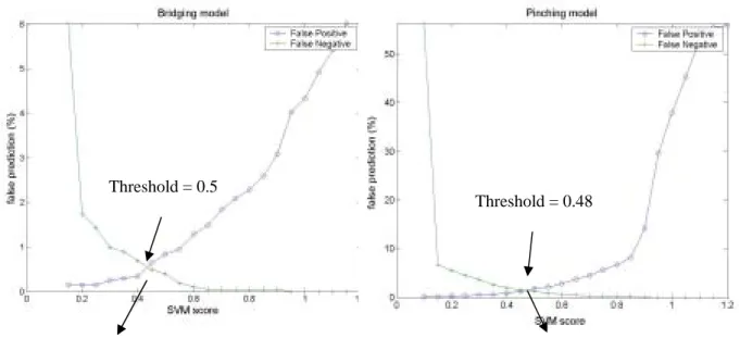
To evaluate the accuracy as well as the best threshold of a CFORC model, bridging and pinching models are applied to the calibration structures. The accuracy of a model is then measured by the number of classification errors, also called false predictions. To do so, we built the ‘false positive / false negative’ curves. Each SVM score lying between 0 and 1 is assumed to be the best threshold value (that is to say the value for which the lowest false prediction rate is obtained). Patterns having a SVM score higher than the SVM threshold under consideration are assumed to fail whereas those having a lower SVM score are assumed to pass. At each threshold the number of false predictions is evaluated: a “false positive” prediction refers to a pattern passing according to the model but failing in reality whereas a false negative prediction refers to a pattern failing according to the model but passing in reality. The intersection of the false positive / false negative curves gives the best threshold, ideally equal to 0.5 with a minimum false predictions rate ideally equal to 0.
The curves (fig 2.3) correspond to the ‘false positive – false negative’ curves obtained with our final CFORC models for pinching and bridging. Both models have a threshold close to 0.5 and a low error rate. Both models accurately predict the printing errors on the calibration test-patterns. Nevertheless, looking back at the model flow if the models were not accurate enough they could be re-generated by changing the optical parameter set, the CFORC model parameters setting (Gaussian standard deviation) or the optical model [3].
The separation between the pass and fail data can be visualized by plotting the line in the 2D case or the surface in the 3D case corresponding to the threshold of 0.5. The following 3D surfaces (fig
2.4)represent the bridging and pinching separation surfaces or the iso-surfaces corresponding to 0.5,
separating passing and failing calibration data.
Threshold = 0.48
False predictions = 1.1 % False predictions = 0.5 %
Threshold = 0.5
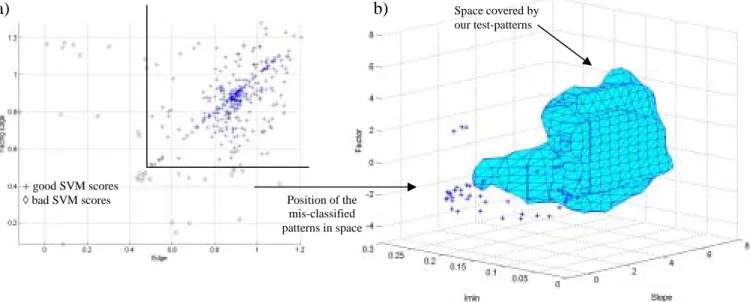
A final accuracy check was done on asymmetrical test-structures. After the SEM observation of the structures across the PW, SVM scores were calculated at failure points on the 2 facing edges. We plot the correspondence between the SVM score of one edge and the SVM score of its facing edge to see if false predictions were occurring. The following plot (fig 2.5 a) concerns experimental pinching failures only and shows that some points are lying in the area where at least one edge has a SVM score below the best threshold. That means that at least one edge will not be tagged by the CFORC pinching model. Plotting those badly classified points into the optical parameter space we saw that this mismatching was due to poor space coverage. Indeed the false predictions belong to structures having optical parameters lying outside the space covered by our test-patterns which is materialized by the plotted surface (fig 2.5 b). This result points out the importance of the parameter space coverage by the calibration data.
Slope
Imax
Slope
Imax
Imin
Factor
◊ passing data
+ failing data
◊ passing data
+ failing data
a) b)
Space covered by our test-patterns + good SVM scores◊ bad SVM scores Position of the
mis-classified patterns in space
Figure 2.5: a) correspondence of SVM scores between an edge and its facing edge on pinching asymmetrical
structures, b) position of the corresponding mis-classified structures in the parameter space.
2.2 Full Process Window model
2.2.1
PW
model
calibration
The full PW model is a compact model similar to OPC models with the main difference being that it is calibrated through dose and focus variations (refer to previous paper [4] [5] for the complete methodology). The main advantage of this technique is that its model building flow is very close to the OPC model building flow (fig 2.6).
The first step of the model building flow is to measure test-patterns at best conditions as well as at several other process conditions. Then optical and resist models are built for the best dose and best focus conditions. The resist model is afterwards applied to the PW data and optimized with this data. If the resist model does not fit the data well, optical and resist models at nominal conditions are re-built.
In our case, the PW model built is calibrated with data measured at best conditions, data measured at ±0.150 µm and ±0.100 µm defocus under best dose condition and data measured ±2.4% dose variation at best focus. The data used for the calibration is similar to the OPC model building data and is composed of 1D and 2D symmetrical patterns.
2.2.2
PW model accuracy
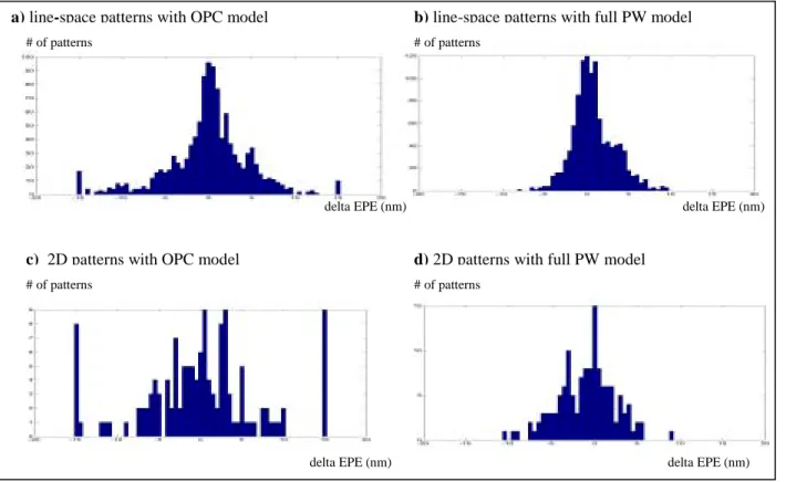
To evaluate PW model accuracy we decided to compare the difference in edge placement error (EPE) between measurements and simulations (called delta EPE) obtained first with our PW model, then with an extended OPC model. This last model is the OPC model calibrated for good CD control at best conditions and used for the regular OPC flow. It is extended to a PW model without optimizing its resist model. OPC and full PW models are applied to the calibration data and to a set of extrapolation data measured at PW corners. The additional data was measured to see if the model could be extrapolated to additional points of the PW. The comparison of delta EPE across PW is done for 1D line-space patterns (a and b fig 2.7) and 2D patterns (c and d fig 2.7). Comparing the delta EPE distributions we see the impact of the PW optimization. Optimizing optical settings and resist model leads to a reduced delta EPE variation across PW.
Figure 2.6: PW model flow
Calibration data measurement across PW Optical and resist models at best conditions Application of resist model to several process conditions PW model Model doesn’t fit calibration data
Model fits optimized
resist model with PW data
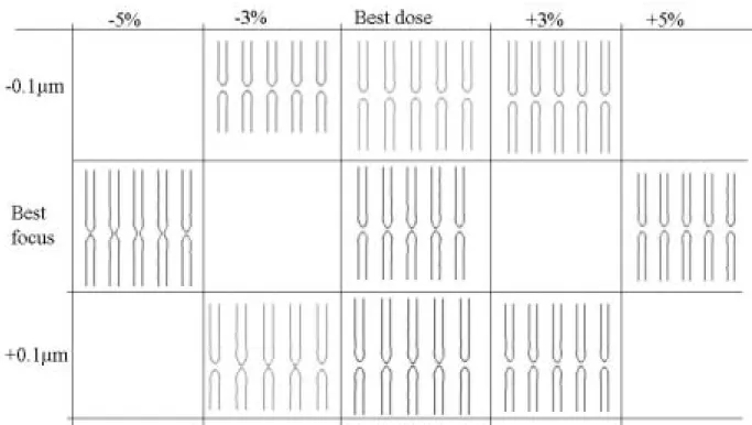
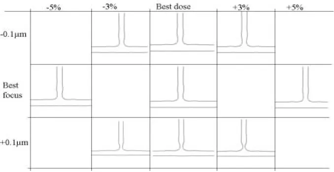
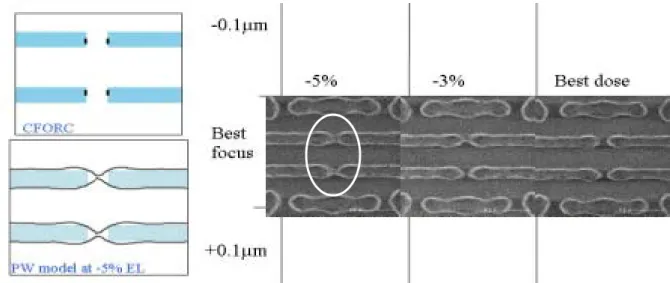
What we are interested in is seeing if our PW model accurately simulates bridging and pinching errors. A comparison between SEM images and corresponding simulated printed images is done across PW for 2 different printing errors: a bridging case on dense line-ends and a pinching case on a T-like structure. The results show that our PW model accurately predicts patterning errors for 2D patterns. For the bridging case SEM images (fig 2.8) show that bridging occurs at best focus with a dose variation of -5%. The corresponding simulations (fig 2.9) show also bridging appearing at this condition.
Figure 2.7: delta EPE across process window comparison for 1D (a & b) and 2D patterns (c & d).
# of patterns # of patterns
# of patterns # of patterns
delta EPE (nm) delta EPE (nm)
delta EPE (nm) delta EPE (nm) a) line-space patterns with OPC model b) line-space patterns with full PW model
c) 2D patterns with OPC model d) 2D patterns with full PW model
For the pinching case, SEM observations (fig 2.10) show that pinching at the T-shape junction is happening at positive defocus whatever the dose value is. Considering the simulation results (fig 2.11) the T-shape structure is resolved at the T-junction across the PW. But at positive defocus, the simulated CD value at the junction is below the fixed CD threshold chosen for the CFORC pinching criteria. Thus structures are also pinching at positive defocus conditions relative to the PW model simulations.
Figure 2.9: Simulated resist images of the dense line-end structure across PW.
3.
Full chip model testing:
3.1 Cycle-time comparison
focus
Simulation points
dose
Pinching simulation points Bridging simulation points
After both models are built and tested, they are applied on the same real post-OPC poly layout to compare their cycle-time. Two different runs will be considered for the full PW model application part. Those runs will be compared in cycle-time to the CFORC run.
The first PW model run consists of simulating pattern shapes at 6 points in the PW (fig 3.1). Those simulation points are the following:
- +5% and -5% EL at best focus, - +3% and -3% at +0.100µm defocus, - +3% and -3% at -0.100µm defocus.
Patterns to be simulated are potential bridging and pinching candidates pre-targeted by geometrical rules. The CFORC run is done on the same patterns. Comparing CPU-time per run, the CFORC run is more than 7 times faster than the first PW run.
The second PW model run consists of sorting bridging and pinching patterns so that simulations on pinching candidates are made at over-exposure conditions and simulations on bridging ones are made at under-exposure conditions (fig 3.2). The cycle-time difference is reduced but the CFORC run is still 4.7 times faster than the PW model based run.
dose
focus
Figure 3.1: simulations points for the 1st run
Figure 3.2: simulation points for the 2nd run Figure 2.11: Simulated resist image of the T-shape structure across PW.
3.2
Predictions comparison
If we compare results given by our 2 runs we see that, based upon the fact that we get a small number of bridging errors, bridging predictions are matching between the 2 methods and correlate to what is printed on wafer. Errors flagged by the full PW model are also flagged by the CFORC (the reverse is not true because CFORC generates some false predictions). The following figure (fig 3.3) is an example of error detection on a SRAM structure.
For the detection of pinching errors, CFORC is accurately predicting pinching errors whereas PW model is missing a lot of pinching errors. The following example (fig 3.4) shows in the same picture an example of pinching error detected by both method and another pinching error detected only by the CFORC method.
Figure 3.3: SRAM bridging predictions versus SEM images
Figure 3.4: Pinching predictions versus SEM images
Best dose
+3%
+5%
Best
focus
-0.1µm
+0.1µm
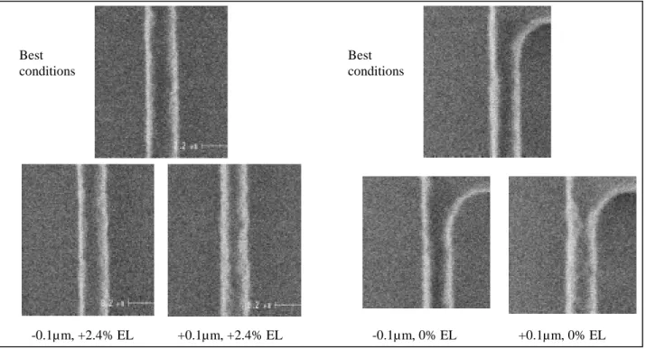
41 nm 44 nmAs the pinching phenomenon is mainly occurring at positive defocus in our study we tried to figure out the reason for PW model mismatch. A potential cause could be the variation of the 3D resist shape through focus. Indeed at positive defocus resist profile is getting sloped. This phenomenon can be seen on SEM images (fig 3.5): the transition between the substrate and the top of the resist is larger at positive defocus. The pinching phenomenon is amplified by the degradation in the resist profile. As CFORC is built on experimental data, it takes into account the 3D resist effect on patterning behavior. Nevertheless the solution for fitting data at positive defocus is to build an extra model calibrated only for positively defocused data and replace the PW model at positive defocus by this extra model.
4.
Conclusion
In this study two different methods were presented and tested for checking pattern robustness across PW: the Critical Failure ORC and the full PW modeling. Regarding to the model building part, both methods required additional work from the conventional OPC model flow, but the PW model flow is quite similar to the OPC model building flow, thus is more easily carried out than the CFORC model flow. Regarding the cycle-time, the CFORC method is less time consuming than full PW model (the CFORC run is more than 4 times faster). Finally, comparing error predictions, PW model is missing real printing issues, whereas CFORC is accurately predicting patterning failures, but with some extra false predictions.
5.
References
[1] “Critical failure ORC –application to the 90nm and 65nm nodes.” J. Belledent, et. al. Proc. of SPIE Vol. 5377, 2004. Best conditions Best conditions -0.1µ m, +2.4% EL +0.1µm, +2.4% EL -0.1µ m, 0% EL +0.1µm, 0% EL
[2] “Failure prediction across process window for robust OPC.” Shumay D. Shang et al. Proc. SPIE, Vol 5040, 2003.
[3] “Lithography yield enhancement through optical rule checking.” J. Word et al. Photonics Asia, 2004.
[4] ”Process window modelling using compact models.” J. A. Torres et al. BACUS, Vol 5567, 2004. [5] “Calibration of OPC models for multiple focus conditions.” J. Schacht et al. Proc. SPIE, Vol 5377, 2004.