Change analysis of dynamic copula for measuring dependence in multivariate financial data

HAL Id: halshs-00189141

https://halshs.archives-ouvertes.fr/halshs-00189141v2

Submitted on 30 Jan 2008

HAL is a multi-disciplinary open access

archive for the deposit and dissemination of sci-entific research documents, whether they are pub-lished or not. The documents may come from teaching and research institutions in France or abroad, or from public or private research centers.

L’archive ouverte pluridisciplinaire HAL, est destinée au dépôt et à la diffusion de documents scientifiques de niveau recherche, publiés ou non, émanant des établissements d’enseignement et de recherche français ou étrangers, des laboratoires publics ou privés.

dependence in multivariate financial data

Dominique Guegan, Jing Zhang

To cite this version:

Dominique Guegan, Jing Zhang. Change analysis of dynamic copula for measuring dependence in multivariate financial data. 2006. �halshs-00189141v2�

Maison des Sciences Économiques, 106-112 boulevard de L'Hôpital, 75647 Paris Cedex 13

http://mse.univ-paris1.fr/Publicat.htm

ISSN : 1624-0340

Centre d’Economie de la Sorbonne

UMR 8174

Change analysis of dynamic copula for measuring dependence in multivariate financial data

Dominique GUEGAN

Jing ZHANG

measuring dependence in multivariate

financial data

D. Gu´egan1 _{and J. Zhang}2?

1 _{Universit´e Paris 1 Panth´eon-Sorbonne, PSE and CES, MSE, 106 Boulevard de}

l’Hˆopital 75013 Paris, France. dguegan@univ-paris1.fr

2 _{Ecole Normale Sup´erieure de Cachan, 94230 Cachan Cedex, France.}

East China Normal University, Department of Statistics, 200063 Shanghai, China. Universit´e Paris 1 Panth´eon-Sorbonne, CES.

celine chang 12@hotmail.com

Abstract. This paper proposes a new approach to measure the depen-dence in multivariate financial data. Data in finance and insurance often cover a long time period. Therefore, the economic factors may induce some changes inside the dependence structure. Recently, two methods using copulas have been proposed to analyze such changes. The first ap-proach investigates the changes of copula’s parameters. The second one tests the changes of copulas by determining the best copulas using mov-ing windows. In this paper we take into account the non stationarity of the data and analyze: (1) the changes of parameters while the copula family keeps static; (2) the changes of copula family. We propose a series of tests based on conditional copulas and goodness-of-fit (GOF) tests to decide the type of change, and further give the corresponding change analysis. We illustrate our approach with Standard & Poor 500 and Nas-daq indices, and provide dynamic risk measures.

Keywords: Dynamic copula; Goodness-of-Fit test; Change-point; Time-varying parameter; VaR; ES.

JEL: C52

1

Introduction

Determining the dependence between assets is an important domain of research. It is useful for portfolio management, risk assessment, option pricing and hedging. The correlation matrices have been a lot considered to quantify the dependence structure between assets,

but it is now well known that this kind of approach is only satis-factory when we work inside a Gaussian or an Elliptical framework.

The recent work ofEmbrechts et al. (2001) proposing the concept of

copulas to measure dependence between financial data has opened the routes to a very interesting research domain, which has shown its ability to improve the domain of quantitative finance.

In the static one-period situation given by the real-valued random

variables X1, · · · , Xd, the dependence between X1, · · · , Xd is

com-pletely determined by their joint distribution function H(X1, · · · , Xd).

The idea of separating H into two parts, one describing the depen-dence structure and the other one describing the marginal behavior

only, leads to the well known concept of copulas, Joe (1997) and

Nelsen (1999). When we adjust copulas on financial data sets, gen-erally we assume strict stationarity all along the considered period,

and we use different criteria such as AIC criterion, Akaike (1974),

D2 diagnostic, Caillault and Gu´egan (2005), to determine the best

one.

Furthermore, most of data sets cover a reasonably long time period and economic factors may induce some changes in the dependence structure: we can observe tranquil periods and turmoil periods for

instance, and then the notion of strict stationarity fails, Gu´egan

(2007). To take into account this phenomenon, the notion of

dy-namic copula has also been introduced in risk management by Dias

and Embrechts (2004),Jondeau and Rockinger (2006), andGranger et al. (2006). The dynamics are introduced inside the copula’s pa-rameters using some time-varying function of predetermined vari-ables. In all these cases the family of the copula remains changeless.

Recently, Caillault and Gu´egan (2007) proposed a new method to

take into account the possibility of changes of the copula’s family and changes inside the parameters, using moving windows. On a se-quence of subsamples, a series of copulas (adjusted with respect to the AIC criterion) are selected. Practically the changes of the copu-las appear evident. However, some problems remain opened such as the choice of the width of the moving window or the detection of the change points. These choices influence the accuracy of the results for

the copula’s adjustment.

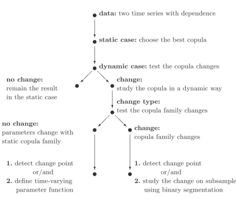
In this paper, we develop a new approach to use the dynamic copula. We proceed in two steps. We test if the copula changes. If not we adjust some dynamics on the parameters of the copula. If the copula changes, we adjust a set of copulas to model the dynamics of the data sets. In order to detect the change type of the copula robustly, we

propose a series of nested tests based on conditional copulas,

Ander-son (1969),Fermanian (2005). Our procedure is as follows. At first, we test whether the copula changes during a considered time period. If the copula seems changeless, we keep the copula and we deal with the changes of copula’s parameters. If we detect some changes in the copulas, then we apply the so called binary segmentation procedure to detect the change time and to build a sequence of copulas. If only the copula parameters change, we apply the change-point analysis

as in Cs¨org˝o and Horv´ath (1997),Gombay and Horv´ath (1999) and

Dias and Embrechts (2004). In this latter case considering that the change-point tests have less power in the case of “small” changes, we assume that the parameters change according to the time-varying functions of some predetermined variables. We summarize our

pro-cedure in Figure 1.

In order to illustrate this new approach, we apply it to Standard & Poor 500 and Nasdaq indices. We study their dynamic dependence and use it for risk management, computing risk measures such as the VaR (Value at Risk) and the ES (Expected Shortfall) measures.

The paper is organized as follows. In Section 2, we review some useful notions and specify the notations. Section 3 presents a series of tests for detecting the copulas’ change. Section 4 analyzes the details for every change type, including the change time, the copulas and the change value of the parameter, etc. In section 5, we provide some empirical research applying the previous method on two real data sets and we associate their dynamic risk measures. Section 6 concludes.

tdata: two time series with dependence

tstatic case: choose the best copula

?

tdynamic case: test the copula changes

? t

no change: remain the result in the static case

¡ ¡

ª _tchange:

study the copula in a dynamic way

@_@R

t

change type:

test the copula family changes

? t

no change:

parameters change with static copula family

¡ ¡ ª

t

1. detect change point or/and 2. define time-varying

parameter function

?

tchange:

copula family changes

@_@R

t

1. detect change point or/and

2. study the change on subsamples using binary segmentation

?

Fig. 1. Change analysis of copula

2

Preliminaries and notations

In order to detect the change of dependence structure, we use con-ditional copulas. Here we simply recall the definitions and introduce some notations. We specify also some assumptions useful in the fol-lowing when we apply the Goodness-of-Fit tests.

2.1 Conditional copulas

Following Patton (2006), the conditional copulas are defined as the

following.

Definition 1. A d-dimensional conditional copula is a function C:

[0, 1]d _{→ [0, 1] such that for some conditioning set F:}

1. For every u = (u1, u2, . . . , ud) ∈ [0, 1]d, C(u|F) = 0 when at

least one coordinate of u is zero, and if all coordinates of u are

2. C is d-increasing conditioned on F,

The Sklar’s theorem (Sklar, 1959) can be extended for conditional

distributions and conditional copulas.

Theorem 1. Let H be a d-dimensional conditional distribution

func-tion with continuous margins F1, F2, · · · , Fd, and let F be some

con-ditioning set, then there exists a unique conditional d-copula C: [0, 1]d

→ [0, 1] such that for all x = (x1, x2, · · · , xd) in R

d

,

H(x|F) = C(F1(x1|F), F2(x2|F), · · · , Fd(xd|F)). (1)

Conversely, if C is a conditional d-copula and F1, F2, · · · , Fd are

univariate conditional distribution functions, then the function H

defined by Equation (1) is a d-dimensional conditional distribution

function with margins F1, F2, · · · , Fd.

2.2 Assumptions and Goodness-of-Fit (GOF) tests

Now we specify some useful assumptions for the GOF tests that we use later. For a d-dimensional stationary process with n

obser-vations (Xn)n∈Z = {(Xi1, Xi2, . . . , Xin) : i = 1, 2, . . . , d}, let H be

its cumulative distribution function. Usually, a GOF test permits to

distinguish between two hypotheses. We denote H0 a known

cumula-tive distribution function, and H = {Hθ|θ ∈ Θ} a known parametric

family of cumulative distribution functions, then the GOF test is:

1. H0 : H = H0, against Ha: H 6= H0, when the null hypothesis is

simple; or

2. H0 : H ∈ H, against Ha : H /∈ H when the null hypothesis is

composite.

We specify now some assumptions:

Assumption 1. Let be K, a probability kernel function on Rd_{, twice}

continuously differentiable, which is the product of d univariate

ker-nels Ki(i = 1, 2, . . . , d) with compact supports.

Assumption 2. Let be hn= (h1n, h2n, . . . , hdn) a bandwidth vector,

nh4+d

n → 0 and nh

3+d/2

n /(ln(ln n))3/2 → ∞ as n → ∞.

Assumption 3. Let be (Xn)n∈Z, we denote ϕn−1= σ((X1,s, X2,s, . . . , Xd,s) :

s ≤ n − 1) the conditional information set available at n − 1 and ϕi,n−1 = σ(Xi,s: s ≤ n − 1) the conditional information set, for the

i-th variable, available at n − 1.

Assumption 4. Let be C0 the true copula associated to (Xn)n∈Z.

For ∀ u ∈ [0, 1]d_{, we denote c}

0 = c0(u, θ) its copula density function,

and θ the parameter vector. In addition, the first two derivatives

of c0 with respect to u are assumed to be uniformly continuous on

Υ (uj) × Υ (θ0), where Υ (uj) represents an open neighborhood of the

points (uj)j=1,2,...,m ∈ [0, 1]d, (m ∈ Z), Υ (θ0) denotes an open

neigh-borhood of θ0.

3

Tests for copula’s change

In this section we use the conditional copulas to perform a series of specified GOF tests.

3.1 Test to detect the change of copula

Using the previous notations and the notion of the conditional cop-ula, we test the null hypothesis,

H(1)₀ : For every n ∈ N, C(·|ϕn−1) = C0(·),

against

H(1)

a : For some n ∈ N, C(·|ϕn−1) 6= C0(·),

where C0 has been introduced before.

In order to apply this test, first we need to build an estimate of

the conditional density c0(uj|ϕn−1) at point uj. We assume that we

observe an n-sample, then its estimate is given by:

ˆc(uj|ϕn−1) = 1 nhd n n X i=1 K(uj − Ui hn ), (2)

where hnand hnare claimed in Assumption 2 and the kernel function

K is claimed in Assumption 1. The vector Ui is such that

Ui = ( ˆF1(X1,i), ˆF2(X2,i), . . . , ˆFd(Xd,i)),

i = 1, 2 . . . , n, where ˆFl is the empirical l-th marginal cumulative

distribution function of (Xn)n∈Z, for l = 1, 2, . . . , d, and

ˆ Fl(Xl,i) = 1 n + 1 n X p=1 1{Xlp<Xli}.

Now we introduce the test statistics:

T = (nhd n) m X j=1 {ˆc(uj|ϕn−1) − c0(uj|ϕn−1)}2 σ2_(u j) , (3)

where σ(uj) satisfies:

σ2_(u

j) = c20(uj|ϕn−1) ·

Z

K2_.

Under the null hypothesis H₀(1), the statistics T defined in Equation

(3) tends to a Chi-square distribution with m degrees of freedom

when n → ∞, Fermanian (2005). Through this test based on T , we

can detect whether or not the copula changes during a considered time period.

Note that the points (uj)j=1,2,...,m ∈ [0, 1]d are chosen arbitrarily.

Clearly, the power of the test T depends on the choice of the points (uj)j=1,2,...,m, which is a drawback as the choice of cells in the usual

GOF Chi-square test. Without a priori, given an integer N, it is

al-ways possible to choose a uniform grid of the type (i1/N, i2/N, . . . , ik/N),

for every integers 1 ≤ i1, i2, . . . , ik ≤ N − 1.

3.2 Test to detect the change type of the copula

If we reject H(1)₀ , then we should study the dependence structure

inside the d-dimensional vector, in a dynamic way. Thus we test the

change type of the copula. Let be C = {Cθ, θ ∈ Θ} a family of

of the process.

Let be the null hypothesis,

H(2)₀ : For every n ∈ N, θn−1 = θ(ϕn−1), C(·|ϕn−1) = Cθn−1 ∈ C,

and the alternative,

H(2)_a : For some n ∈ N, C(·|ϕn−1) /∈ C.

We use the same notations as before and we introduce the statistics associated to this test:

R = (nhd_n) m X j=1 {ˆc(uj|ϕn−1) − c_θˆ_n−1(uj|ϕn−1)}2 ˆ σ2_(u j) , (4)

where uj (j = 1, 2, . . . , m) is described in Assumption 4, the

σ-algebra ϕn−1 is introduced in Assumption 3, and ˆθn−1 is the

con-sistent estimator of θn−1. c_θˆ_n−1(uj|ϕn−1) denotes the density of the

conditional copula C_θˆ_n−1, and ˆc(uj|ϕn−1) is the empirical copula

den-sity given in Equation (2). Moreover,

ˆ

σ2_(u

j) = c2_θˆ_n−1(uj|ϕn−1) ·

Z

K2_.

Under the null hypothesis H(2)₀ , the statistics R defined in Equation

(4) tends to a Chi-square distribution with m degrees of freedom,

when n → ∞. If we reject H(2)₀ , the copula family changes. On the

other hand, if we do not reject H(2)₀ , the copula family remains static,

then we say that only the copula’s parameters change. After

deter-mining the change type of the copula by testing H(2)₀ , we analyze in

details the copula’s changes.

Note that if we consider the Archimedean copula family C = {Cθ, θ ∈

Θ}, the parameter θ can be estimated using the Kendall’s tau.

4

Detail analysis for the copula change

According to the test results for the hypotheses H(1)₀ and H(2)₀ , we

determine the change type of the copula during the time period. Here, we analyze two kinds of changes.

4.1 Detail analysis for the change of copula’s family

If we reject H(2)₀ , then the copula’s family may change. We apply the

so called binary segmentation procedure to detect the change point.

This procedure proposed byVostrikova (1981) enables to

simultane-ously detect the number and the location of the change-points. The procedure can be described as follows. Firstly, we choose the best copula according to the AIC criterion on the whole sample. Then the sample is divided into two subsamples, we choose the best cop-ulas on these two subsamples respectively. If the two best copcop-ulas are different from the copula on the whole period, we continue this segmentation procedure, i.e., we again divide each subsample into two parts, and do the same work as in the previous step. Finally, the procedure stops when all the best copulas on the subsamples have been adjusted. Therefore, we get all the change points for the family changes.

4.2 Detail analysis for the change of copula’s parameters

If H₀(2)is not rejected, the copula’s family remains changeless.

There-fore, we say that only the copula parameters change. Then, we need to deal with the change analysis for the parameters.

To find the change time, we apply the change point technique

intro-duced byDias and Embrechts(2004). Let u1, · · · , unbe a sequence of

independent random vectors in [0, 1]d_{with univariate uniformly}

dis-tributed margins and copulas C(u; θ1, η1), · · · , C(u; θn, ηn),

respec-tively, where θi and ηi represent the dynamic and the static copula

parameters satisfying θi ∈ Θ(1) ⊆ Rp and ηi ∈ Θ(2) ⊆ Rq. We test

the null hypothesis

H(3)₀ : θ1 = θ2 = . . . = θn and η1 = η2 = . . . = ηn

against

H(3)_a : θ1 = . . . = θk∗ 6= θ_k∗₊₁ = . . . = θ_n and η₁ = η₂ = . . . = η_n.

Here k∗ _{is the location or time of the change-point if we reject the}

likelihood ratio, that is, the null hypothesis would be rejected for small values of the likelihood ratio:

Λk = sup_(θ,η)∈Θ(1)_×Θ(2) Q 1≤i≤nc(ui; θ, η) sup_(θ,θ0_,η)∈Θ(1)_×Θ(1)_×Θ(2) Q 1≤i≤kc(ui; θ, η) Q k<i≤nc(ui; θ0, η) ,

where c is the density of C. The statistic Λk is carried out through

maximum likelihood method, all the necessary conditions of

regular-ity and efficiency have to be assumed,Lehmann and Casella (1998).

If Lk(θ, η) =

P

1≤i≤klog c(ui; θ, η), and L∗k(θ, η) =

P

k<i≤nlog c(ui; θ, η),

then, the likelihood ratio equation can be written as

−2 log(Λk) = 2(Lk(ˆθk, ˆηk) + L∗k(θ∗k, ˆηk) − Ln(ˆθn, ˆηn)).

The hypothesis H(3)₀ is rejected for large values of

Zn= max

1≤k<n(−2 log(Λk)).

PursuingGombay and Horv´ath (1996), the following approximation

holds: P(Z1/2 n ≥ x) ≈ xp_exp(−x2_/2) 2p/2_{Γ (p/2)} · (HL − p x2HL + 4 x2 + O( 1 x4)), as x → ∞, where HL = log(1 − gn)(1 − ln) gnln , gn= ln = (log n)3/2/n,

Dias and Embrechts (2004).

If we assume that there is exactly one change point, then the

esti-mate for the change time is given by ˆkn = min{1 ≤ k < n : Zn =

−2 log(Λk)}.

Considering that the change-point test has less power for small changes, we analyze the dependence more specifically by assuming a time-varying behavior for the corresponding parameter. In order to show how it works, we provide now the dynamics of the parameters for the copulas that we use in the applications. The definitions of the copulas are recalled in an Annex.

Using the dynamic Gaussian copula, we define the dynamic correla-tion as :

ρt= h−1(r0+ r1x1,t−1x2,t−1+ s1h(ρt−1)), (5)

where (x1,t)tand (x2,t)tare the samples, r0, r1, s1 the parameters and

h(·) the Fisher’s transformation such that h(ρ) = log(1+ρ_1−ρ), to ensure

that −1 < ρ < 1.

If we work with the dynamic Student t-copula, the dynamic degrees of freedom ν can be defined as:

νt = l−1(r0+ r1x1,t−1x2,t−1+ s1l(νt−1)), (6)

where r0, r1, s1 are parameters and l(·) is a function defined as:

l(ν) = log( 1

ν−2).

For the dynamic Gumbel copula, the dynamic parameter δ can be described as:

δt= w−1(r0+ r1x1,t−1x2,t−1+ s1w(δt−1)), (7)

where r0, r1, s1 are parameters and w(·) is a function defined as:

w(δ) = log( 1

ν−1).

5

Empirical work

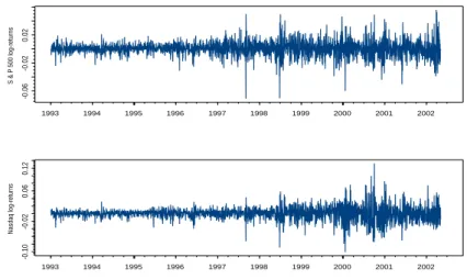
We apply now the above change analysis of dynamic copula to Stan-dard & Poor 500 (S&P500) and Nasdaq indices. The sample data sets contain 2436 daily observations from 4 January, 1993 to 30 Au-gust, 2002 for both assets. The log-returns of these two indices are

shown in Figure 2.

From Figure 2, it is observed that the outliers of the two underlying

log-returns typically occur simultaneously, and almost in the same direction. We observe that both assets fluctuate a lot from the mid-dle of 1997 when the Asian financial crisis burst out.

S & P 500 log-returns 1993 1994 1995 1996 1997 1998 1999 2000 2001 2002 -0.06 -0.02 0.02 Nasdaq log-returns 1993 1994 1995 1996 1997 1998 1999 2000 2001 2002 -0.10 -0.02 0.06 0.12

Fig. 2. Log-returns for S&P500 (up) and Nasdaq (down) Indices

Let ri,t(i = 1, 2) be the daily log-returns for S&P500 and Nasdaq

respectively. In order to filter the observed instability, we fit a uni-variate GARCH(1,1) model to each log-return series, that is:

ri,t = µi+ ξi,t with ξi,t = σi,tεi,t,

σ2

i,t = αi,0+ αi,1ε2i,t−1+ βi,1σ2i,t−1,

εi,t|ϕi,t−1∼ N(0, 1),

(8)

where µi is the drift, αi,0, αi,1, βi,1 are parameters in R. The

estima-tion of the parameters using likelihood method are given in Table1.

Table 1. Estimates of GARCH(1,1) parameters

Parameter S&P500 Nasdaq

µ 6.013e-04 (1.633e-04) 9.395e-04 (2.116e-04)

α0 6.018e-07 (1.579e-07) 1.486e-06 (2.877e-07)

α1 7.947e-02 (6.670e-03) 1.157e-01 (8.902e-03)

β1 9.201e-01 (6.761e-03) 8.849e-01 (8.596e-03)

5.1 Dynamic copula for S&P500 and Nasdaq indices In order to investigate the dependence between these two data sets, we firstly adjust the best copula for the standard residual-pairs

(ε1,t, ε2,t) over the whole period using AIC criterion. The set of

ulas includes Gaussian, Student t, Gumbel, Clayton and Frank

cop-ulas. The copulas fitting is given in Table 2. Although Student t

copula has the smallest AIC value, the estimation is unfortunately not convergent, therefore, Gaussian copula provides the best copula for the whole sample.

Table 2. Copula fitting results

Copula Parameter AIC Convergence Gaussian 8.116e-01 (2.684e-02) -2615.196 T Student t 8.143e-01 (3.384e-02);

13.668 (5.078e-01) -2642.88 F Gumbel 2.461 (4.090e-02) -2505.374 T Clayton 1.659 (5.280e-02) -1867.982 T Frank 8.391 (1.878e-01) -2419.844 T

Figures in brackets are standard errors, for Student t copula, the first parameter is correlation, the second one is degree of freedom, and “T” means “True”, “F” means “Fault”.

In a first step, we test the stability of this copula. We use the test

developed in Section 3.1 and the statistics T in Equation (3). Here,

we assume that the true copula is the Gaussian one specified in Table

2. To apply the test, we choose a kernel function K given by

K(u) = (15 16) 2 2 Y i=1 (1 − u2 i)21{ui∈[0,1]}, a bandwith ˆhn = p (σ2 1 + σ22)/2 n1/6 , and σ 2

l will be the empirical

vari-ance of ˆFl (l = 1, 2). Furthermore, for the points (uj)j=1,2,...,m in

Assumption 4, we choose m = 81 points on the uniform grid with the type of (1/10, 2/10, . . . , 9/10) × (1/10, 2/10, . . . , 9/10).

Using this approach, the p-value for the null hypothesis H(1)₀ is equal to 0. Thus the null hypothesis is rejected and the copula for the data set does not remain static.

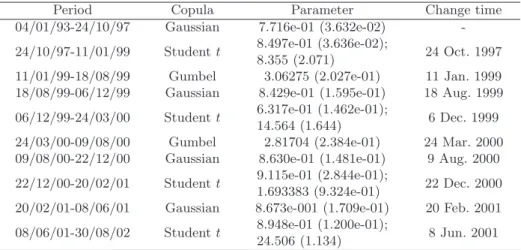
In a second step, we detect the changes of copula’s family using

the binary segmentation procedure described in Section 4.1. Trough

deciding the best copulas on the subsamples divided by the binary segmentation, all of the change time for the copula’s family are

de-tected. The results are given in Table 3.

Table 3. Changes of copula’s family

Period Copula Parameter Change time 04/01/93-24/10/97 Gaussian 7.716e-01 (3.632e-02) -24/10/97-11/01/99 Student t 8.497e-01 (3.636e-02);

8.355 (2.071) 24 Oct. 1997 11/01/99-18/08/99 Gumbel 3.06275 (2.027e-01) 11 Jan. 1999 18/08/99-06/12/99 Gaussian 8.429e-01 (1.595e-01) 18 Aug. 1999 06/12/99-24/03/00 Student t 6.317e-01 (1.462e-01);

14.564 (1.644) 6 Dec. 1999 24/03/00-09/08/00 Gumbel 2.81704 (2.384e-01) 24 Mar. 2000 09/08/00-22/12/00 Gaussian 8.630e-01 (1.481e-01) 9 Aug. 2000 22/12/00-20/02/01 Student t 9.115e-01 (2.844e-01);

1.693383 (9.324e-01) 22 Dec. 2000 20/02/01-08/06/01 Gaussian 8.673e-001 (1.709e-01) 20 Feb. 2001 08/06/01-30/08/02 Student t 8.948e-01 (1.200e-01);

24.506 (1.134) 8 Jun. 2001 “Period” shows the start and end time of the observations within the corresponding subsamples, in the form of Day/Month/Year, where “Year” is represented by the last two numbers of the year, i.e., “99” represents the year 1999 for instance. Figures in brackets are standard errors, and for Student t copula, the first parameter is correlation, the second one is degree of freedom.

The result in Table3 provides the change period for copula’s family

that coincide with some financial incidents:

– 24 Oct. 1997: copula family changes from Gaussian to Student

t. This date corresponds to 27 October, 1997 when the Asian financial crisis came to a head.

– 11 Jan. 1999: copula family changes from Student t to Gumbel. This date corresponds to the introduction of Euro as the unit European currency.

– 24 Mar. 2000: copula family changes from Student t to

Gum-bel. This date corresponds to the technology-heavy Nasdaq stock market peaked on 10 Mar. 2000 and S&P 500 peaked on 24 Mar. 2000.

– 8 Jun. 2001: copula family changes from Gaussian to Student

t. This date corresponds to the subsequent 9.11 attacks and the recession lasted from March 2001 to November 2001 in the United States.

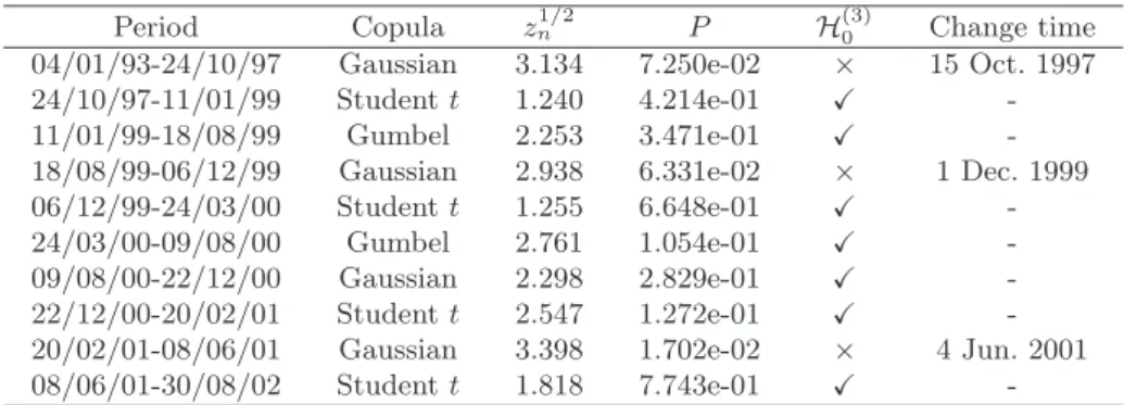
Thirdly, for each corresponding period within which the copula’s family does not change, we detect the change points for the copula’s

parameters in the way introduced in Section 4.2. We provide the

re-sults in Table 4. zn1/2 is the corresponding observation value for the

statistics Zn1/2.

Table 4. Change-point for copula’s parameters

Period Copula zn1/2 P H(3)0 Change time

04/01/93-24/10/97 Gaussian 3.134 7.250e-02 × 15 Oct. 1997 24/10/97-11/01/99 Student t 1.240 4.214e-01 X -11/01/99-18/08/99 Gumbel 2.253 3.471e-01 X -18/08/99-06/12/99 Gaussian 2.938 6.331e-02 × 1 Dec. 1999 06/12/99-24/03/00 Student t 1.255 6.648e-01 X -24/03/00-09/08/00 Gumbel 2.761 1.054e-01 X -09/08/00-22/12/00 Gaussian 2.298 2.829e-01 X -22/12/00-20/02/01 Student t 2.547 1.272e-01 X -20/02/01-08/06/01 Gaussian 3.398 1.702e-02 × 4 Jun. 2001 08/06/01-30/08/02 Student t 1.818 7.743e-01 X -“Period” shows the start and end time of the observations within the corresponding subsamples, in the form of Day/Month/Year, where “Year” is represented by the last two numbers of the year, i.e., “99” represents the year 1999 for instance. P denotes the probability P (Zn1/2> zn1/2) in Section4.2, the null hypothesis H(3)0 is rejected at a

10% level, we simply denote “X” as “not reject” and “×” as “reject”.

The change points for the copula’s parameter shown in Table4reflect

– 15 Oct. 1997: corresponds to the Asian financial crisis beginning from July 1997;

– 1 Dec. 1999: corresponds to the preparation of the unit European

currency, euro;

– 4 Jun. 2001: corresponds to the recession beginning from March

2000 to November 2001, as the real gross domestic product in the United States dropped by 0.2% total from the fourth quarter of 2000;

Finally, as the above change-point analysis only detects “large” changes in the parameters, we further study the dynamic parameters using

the appropriate time-varying functions introduced in Equation (5),

(6) and (7). The results are given in Table 5.

5.2 Risk management strategy

Our systematic change analysis for the dynamic copula can be tractably applied to measure the dynamics in the dependence structure of the financial data. Now we compute the simulated VaR and ES mea-sures in a dynamic way. For a given probability level α, 0 < α < 1,

VaRα is simply the maximum loss that is exceeded over a specified

period with a level of confidence 1 − α. If X is a random return with

distribution function FX, then

FX(VaRα) = P {X ≤ VaRα} = α.

Thus, losses lower than VaRαoccur with probability α. For the other

measure ES (Expected Shortfall), it represents the expectation of

loss knowing that a threshold is exceeded, for instance VaRα, and

we define it as:

ESα(X) = E{X|X ≤ VaRα}.

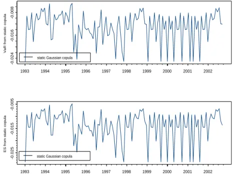
For the portfolio of S&P500 and Nasdaq with equal weight, we com-pare the VaR and ES values using the static copula and the dynamic copula. For the static copula, we choose the Gaussian copula given

in Table 2 corresponding to the whole period. We use the dynamic

copula obtained through time-varying parameters (given in table5)

Table 5. Estimates for time-varying parameters

Period Copula Parameter r0 r1 s1

04/01/93-24/10/97 Gaussian dynamic ρ 2.620e-02 (4.961e-02) 4.160e-02 (5.347e-02) 9.735e-01 (2.689e-01) 24/10/97-11/01/99 Student t ρ = 8.249e-01 (2.264e-02) ; - - -dynamic ν 8.915e-01 (8.238e-01) -1.632e-01 (1.389e-01) 3.313e-01 (1.226e-01) 11/01/99-18/08/99 Gumbel dynamic δ -1.263 (2.194e-01) -5.236e-03 (1.129e-01) -7.700e-01 (3.890e-02) 18/08/99-06/12/99 Gaussian dynamic ρ 3.266 (1.495) 3.081e-02 (3.636e-03) -3.557e-01 (3.291e-02) 06/12/99-24/03/00 Student t ρ = 5.433e-01 (2.938e-02) ; - - -dynamic ν 7.228e-01 (5.977e-01) 4.033e-01 (1.428e-01) -6.784e-01 (2.584e-01) 24/03/00-09/08/00 Gumbel dynamic δ -8.134e-01

(5.823e-01) -3.892e-02 (3.937e-01) -4.400e-01 (5.333e-02) 09/08/00-22/12/00 Gaussian dynamic ρ 3.317 (3.055e-02) 1.104e-01 (2.343e-03) -3.147e-01 (7.314e-01) 22/12/00-20/02/01 Student t ρ = 9.387e-01 (5.236e-01) ; - - -dynamic ν -1.922 (1.485) 1.276 (1.893) -5.806e-01 (5.530e-01) 20/02/01-08/06/01 Gaussian dynamic ρ 4.236e-02

(6.874e-01) 3.808e-02 (5.258e-02) 9.792e-01 (2.180e-01) 08/06/01-30/08/02 Student t ρ = 8.747e-01 (2.711e-02) ; - - -dynamic ν -5.764e-01 (5.540e-01) -3.595e-01 (8.683e-01) -1.025 (3.303e-01) “Period” shows the start and end time of the observations within the corresponding subsamples, in the form of Day/Month/Year, where “Year” is represented by the last two numbers of the year, i.e., “99” represents the year 1999 for instance. Figures in brackets are standard errors.

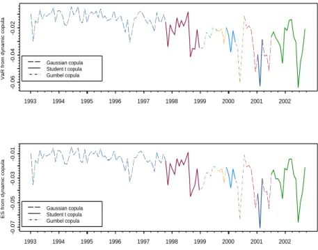
change in each subsample (the families of copulas are provided in

Ta-ble 3). We calculate the VaR and ES values per 20 days in order to

clearly observe the dynamics. The results obtained from the static

and dynamic copulas are shown in Figure 3 and Figure4.

VaR from static copula

1993 1994 1995 1996 1997 1998 1999 2000 2001 2002

-0.024

-0.016

-0.008

static Gaussian copula

ES from static copula

1993 1994 1995 1996 1997 1998 1999 2000 2001 2002

-0.025

-0.015

-0.005

static Gaussian copula

Fig. 3. VaR and ES using static copula for the portfolio of S&P500 and Nasdaq Indices

From Figure 3 and Figure 4, it can be observed that the VaR and

ES values fluctuate a lot. Through comparison, some conclusions are summarized below:

1. The dynamics of the VaR and ES using the static copula only

come from the volatilities of the GARCH model, while using the dynamic copulas, the dynamics of VaR and ES still depend on the dynamic dependence structure;

VaR from dynamic copula 1993 1994 1995 1996 1997 1998 1999 2000 2001 2002 -0.06 -0.04 -0.02 Gaussian copula Student t copula Gumbel copula

ES from dynamic copula

1993 1994 1995 1996 1997 1998 1999 2000 2001 2002 -0.07 -0.05 -0.03 -0.01 Gaussian copula Student t copula Gumbel copula

Fig. 4. VaR and ES using dynamic copulas for the portfolio of S&P500 and Nasdaq Indices

2. The VaR and ES from the static copula have generally smaller

ab-solute values than those from the dynamic copulas, which means that the dynamic copula model shows more risk information than the static one. It is very important for portfolio investors who al-ways choose the portfolio with the smallest VaR and ES absolute values. In practice, we observed that it is not appropriate to com-pute the VaR and ES values using the static copula.

3. After the middle of 1997 when the Asian financial crisis broke out,

the VaR and ES values calculated from the dynamic copula vary a lot, while this phenomenon does not distinctly appear when we use the static copula. This means that the dynamic copula model proves better than the static one in terms of the sensitivity to the risk .

From the above remarks, it appears that the dynamic changes in-side the dependence structure of a portfolio plays an important role in risk management. Recently we have also observed this fact in multivariate option pricing, using dynamic dependence measured by

copulas, Gu´egan and Zhang (2007).

6

Conclusion

In this paper, we introduce a new approach to detect the best dy-namic copula which characterizes the evolution of several data sets. It is based on a series of nested tests concerning the conditional copula and the GOF test. This approach permits to determine the change type of the copula using the binary segmentation procedure, the change-point analysis and the time-varying parameter functions. We illustrate our approach with S&P500 and Nasdaq indices. The empirical result presented the changes of copula’s family as well as the changes of parameters. Furthermore, our approach has been ap-plied to give the dynamic risk measures VaR and ES, which plays an important role in risk management.

7

Annex

7.1 Gaussian copula

The copula of the d-variate normal distribution with linear correla-tion matrix R is

CGa_R (u) = Φd

R(Φ−1(u1), Φ−1(u2), · · · , Φ−1(ud)),

where Φd

R denotes the joint distribution function of the d-variate

standard normal distribution function with linear correlation

ma-trix R, and Φ−1 _{denotes the inverse of the distribution function of}

the univariate standard Gaussian distribution. Copulas of the above form are called Gaussian copulas. In the bivariate case, we denote ρ as the linear correlation coefficient, then the copula’s expression can be written as CGa(u, v) = Z _Φ−1_(u) −∞ Z _Φ−1_(v) −∞ 1 2π(1 − ρ2₎1/2 exp{− s2_{− 2ρst + t}2 2(1 − ρ2₎ }dsdt.

The Gaussian copula CGa with ρ < 1 has neither upper tail depen-dence nor lower tail dependepen-dence.

7.2 Student-t copula

If X has the stochastic representation

X= µ +d

√ ν √

SZ, (9)

where= represents the equality in distribution or stochastic equality,d

µ ∈ Rd_{, S ∼ χ}2

ν and Z ∼ Nd(0, Σ) are independent, then X has a

d-variate tν distribution with mean µ (for ν > 1) and covariance matrix

ν

ν−2Σ (for ν > 2). If ν ≤ 2 then Cov(X) is not defined. In this case

we just interpret Σ as the shape parameter of the distribution of X.

The copula of X given by Equation (9) can be written as

Ct

ν,R(u) = tdν,R(t−1ν (u1), t−1ν (u2), · · · , t−1ν (ud)),

where Rij = Σij/

p

ΣiiΣjj for i, j ∈ {1, 2, · · · , d}, tdν,R denotes the

distribution function of √νY/√S, S ∼ χ2

ν and Y ∼ Nd(0, R) are

independent. Here tν denotes the margins of tdν,R, i.e., the distribution

function of √νYi/

√

S for i = 1, 2, · · · , d. In the bivariate case with the linear correlation coefficient ρ, the copula’s expression can be written as Ct ν,R(u, v) = Z _t−1 ν (u) −∞ Z _t−1 ν (v) −∞ 1 2π(1 − ρ2₎1/2{1+ s2_{− 2ρst + t}2 ν(1 − ρ2₎ } −(ν+2)/2_dsdt.

Note that ν > 2. And the upper tail dependence and the lower tail dependence for Student t copula have the equal value.

7.3 Gumbel copula

The Gumbel copula is defined as

CGu(u, v; δ) = exp{−[(− ln u)δ+ (− ln v)δ]1/δ}, δ ∈ [1, ∞).

1. δ = 1 implies CGu(u, v; 1) = uv;

2. As δ → ∞, CGu(u, v; δ) → min(u, v);

3. Gumbel copula has upper tail dependence: 2 − 21/δ_;

4. Gumbel copula has no lower tail dependence.

The Gumbel copula belongs to the Archimedean copula,Joe (1997)

Akaike, H., 1974. A new look to the statistical model identification. IEEE Transactions on Automatic Control, AC-19, 716-723. Anderson, T. W., 1969. Statistical inference for covariance matrices

with linear structure. Proceeding in the Second International Sym-posium on Multivariate Analysis, ed. P. R. Krishnaiah. Academic Press, New York, 55-66.

Caillault, C. and Gu´egan, D., 2007. Forecasting VaR and Expected Shortfall using dynamical systems: A risk management strategy, Frontiers in Finance, to appear.

Caillault, C., Gu´egan, D., 2005. Empirical estimation of tail depen-dence using copulas: Application to Asian markets. Quantitative Finance, 5, 489-501.

Cs¨org˝o, M., Horv´ath, L., 1997. Limit Theorems in Change-point Analysis. Wiley, Chichester.

Dias, A., Embrechts, P., 2004. Dynamic copula models for multivari-ate high-frequency data in finance. Manuscript, ETH Zurich. Embrechts, P., McNeil, A., Strausmann, D., 2001. Correlation and

dependence in risk management: properties and pitfalls. Risk Man-agement: Value at Risk and Beyond, ed. M.A.H. Dempster, Cam-bridge University Press, 176-223.

Fermanian, J-D., 2005. Goodness of fit tests for copulas. Journal of multivariate analysis 95, 119-152.

Gombay, E., Horv´ath, L., 1996. On the rate of approximations for maximum likelihood test in change-point models. Journal of Mul-tivariate Analysis 56, 120-152.

Gombay, E., Horv´ath, L., 1999. Change-points and bootstrap. Envi-ronmetrics 10, 725-736.

Granger, C.W.J., Ter¨asvirta, T., Patton, A. J., 2006. Common fac-tors in conditional distributions for bivariate time series. Journal of Econometrics 132, 43-57.

Gu´egan, D., 2007. Global and local stationary modelling in finance: Theory and empirical evidence. Working Paper, CES, Universit´e Paris 1 Panth´eon - Sorbonne,France, 2007.54.

Gu´egan, D., Zhang, J., 2007. Pricing Bivariate Option under GARCH-GH Model with Dynamic Copula: Application for

Chinese Market, Working Paper, CES, Universit´e Paris 1 Panth´eon -Sorbonne, france, 2007.57.

Joe, J., 1997. Multivariae Models and Dependence Concepts. Chap-man & Hall, London.

Jondeau, E., Rockinger, M., 2006. The copula-GARCH model of con-ditional dependencies: An international stock market application. Journal of International Money and Finance 25, 827-853.

Lehmann, E. L., Casella, G., 1998. Theory of point estimation, sec-ond edition. Springer, New York.

Nelsen, R., 1999. An introduction to copulas. Lecture Notes in Statis-tics 139.

Patton, A. J., 2006. Modelling asymmetric exchange rate depen-dence. International Economic Review 47, 527-556.

Silverman, B. W., 1986. Density Estimation for Statistics and Data Analysis. Chapman & Hall, CRC.

Sklar, A., Fonctions de r´epartition `a n dimensions et leurs marges. Publications de l’Institut de Statistique de L’Universit´e de Paris. 8, 229-231.

Vostrikova, L. J.,1981. Detecting “disorder” in multidimensional ran-dom processes. Soviet Mathematics Doklady 24, 55-59.