HAL Id: hal-00076898
https://hal.archives-ouvertes.fr/hal-00076898
Submitted on 3 Sep 2006
HAL is a multi-disciplinary open access
archive for the deposit and dissemination of sci-entific research documents, whether they are pub-lished or not. The documents may come from teaching and research institutions in France or
L’archive ouverte pluridisciplinaire HAL, est destinée au dépôt et à la diffusion de documents scientifiques de niveau recherche, publiés ou non, émanant des établissements d’enseignement et de recherche français ou étrangers, des laboratoires
Numerical method for the Compton scattering operator.
Christophe Buet, Stéphane Cordier
To cite this version:
Christophe Buet, Stéphane Cordier. Numerical method for the Compton scattering operator.. Se-ries on Advances in Mathematics for Applied Sciences, 2003, Lectures notes on discretization of the Boltzmann equation, pp.63. �hal-00076898�
Numerical method for the Compton scattering
operator.
C. Buet
1, S. Cordier
21Commissariat `a l’´Energie Atomique, 91680 Bruy`eres-le-Chˆatel email [email protected]
2 Laboratoire MAPMO, UMR 6628,
Universit´e Orl´eans, 45067 Orl´eans, France email [email protected]
Abstract In this paper, we present a new discretization of the Kompaneets equation. This equation can be derived from the Quantum Boltzmann equation for cross sections localized around small changes in the energy. The two collision operators share the same properties (conservation, entropy and steady states). The numerical methods are designed in order to preserve these properties which insures the correct long time behaviour. A supplementary difficulty arises for initial data with a density larger than a critical one, associated with a Planck distribution. In this case, the equilibrium state are the sum of a smooth Planck distribution plus a Delta measure on zero energy. The scheme is able to deal with this singularity.
1
Introduction
We are interested in the dynamics of a low energy, homogeneous and isotropic photon gas that interacts via Compton scattering with a low energy electron gas in thermodynamical equilibrium.
In this paper, we first review the main properties of the Quantum Boltzmann equation (QBE) and its ”grazing” collision limit that is called the Kompaneets equation (which is a Fokker-Planck like equation). We will recall recent result of Escobedo and Mischler [EM, EM2] about the equilibrium state of such equation that behaves under some conditions as a ”concentration near the origin” (section 2).
In section 3.1, we present a numerical scheme for the QBE that preserves the properties of the equation described above.
Then, we present a numerical scheme for the Kompaneets equations that has the same properties i.e. are compatible with all the properties of the continuous equation. This allow us to observe the ”concentration” phenomena. We present two ways for deriving this scheme . The first way is based on the asymptotic that transform the QBE into the Kompaneets equation at the discrete level. The second one is based on the same ideas as the Chang-Cooper paper [CC] . These two methods lead surprisingly to the same scheme up to a multiplicative constant (that goes to 1 when the mesh is refined) and this fact allows us to use either method usually devoted to Boltzmann like equation (e.g. entropy decay) or to Fokker-Planck type equation (Maximum principle).
We shall also deal with the difficulty due to the mass concentration phenom-ena. For this, we shall defined generalized Bose-Einstein distribution function (with negative value of ν) that converge (when the mesh is refined) toward the Planck distribution plus a Dirac measure at origin.
We then illustrate the schemes on the following result by Escobedo et al. [E3] : even if the initial density is smaller than the Planck one, the solution of the Kompaneets equation (with the boundary conditions) is not always global in time (on the contrary, the solutions of the QBE are well defined for any time) provided that the initial density (arbitrary small) is close enough to the origin. This is due to a balance between the ”Burgers” term (with a negative velocity that push the particle toward the origin and the diffusion term that spreads the solution. We shall observe this ”blow-up” in finite time.
This paper is related to previous works of the authors on the Boltzmann or Fokker-Planck-Landau operator [BCDL, BC] . In these papers, numerical discretizations are designed in order to be compatible with relevant physical properties such as conservation laws and entropy decay using Discrete Veloci-ties Method. These methods allow to insure the correct large time behaviour i.e. the trend to thermodynamical equilibrium. The numerical efficiency of the proposed algorithms have been tested also for the non homogeneous case (where the distribution function depend on the space variable too) in a paper by the authors and F. Filbet [BCF] .
2
Quantum Boltzmann and Kompaneets
Equa-tion
In this section, we briefly present the equation we are interested in, namely the Quantum Boltzmann equation and its ”grazing” limit the so called
Kom-paneets equation. We refer to [K] for the original paper on these equations and to [EM, EM2] for a more recent and mathematical presentation.
2.1
The Quantum Boltzmann Equation
We consider an isotropic and homogeneous photon gas scattered by cold electrons at thermodynamical equilibrium. The distribution function of the photons f depends on time and on the energy variable k : f (k, t) represents the number of photons that have energy k ≥ 0 at time t ≥ 0. This function f obeys to the following scaled quantum Boltzmann equation (QBE)
k2∂f ∂t = ! ∞ 0 b(k" , k)(f" (1 + f ) exp(−k) − f (1 + f" ) exp(−k" ))dk" , (2.1)
where we omit the variable k and t for simplicity and f" as usual denotes f (k", t). The so called cross section b - positive and symmetric- is related to the probability for a given particle at energy level k to be scattered to the energy level k". The exponential terms represents the distribution function of electrons. Defining g = k2f , equation (2.1) can be rewritten as
∂g ∂t =
! ∞
0
b(k", k)(g"(k2+ g) exp(−k) − g(k"2+ g") exp(−k"))dk", (2.2) Let us define the function h of two variable as
h(g, k)def= g
k2+ g. (2.3)
In the reminder, we shall also note h = h(g, k) = h(g(k), k). Using this notation, the QBE equation (2.2) reads in the more symmetric form
∂g ∂t = ! ∞ 0 b(k" , k)ekek!(k2+ g)(k"2 + g" )(h(g" , k" )ek!− h(g, k)ek)dk" , (2.4)
In the reminder of the paper, we write QB for the Quantum Boltzmann operator defined above as the right hand side in (2.4).
Multiplying (2.4) by a test function Ψ(k), integrating over k and replacing k by k", we have the weak symmetrized formulation of the QB operator
! ∞ 0 ∂g ∂tΨ(k)dk = 1 2 ! ∞ 0 ! ∞ 0 (Ψ(k) − Ψ(k" )) b(k" , k)e−ke−k! (2.5) (k2+ g)(k"2+ g")(h(g", k")ek! − h(g, k)ek)dk"dk.
Using this weak formulation, one obtains easily the unique law of conservation for the QBE, that is the conservation of the total density
N def= N(g) =
! ∞
0
gdk, d
dtN(g) = 0. (2.6)
The second main property of the QBE is the decay of entropy. We first define the function s(x, k) of two variables as
s(x, k)def= x log(x) + k2log(k2) + kx − (k2+ x) log(k2+ x), and thefunctional entropy, H as
H(g)def=
! ∞
0
s(g(k), k)dk (2.7)
Then, H decays in time
d
dtH ≤ 0.
This property, so called H-theorem can be easily checked, at least formally, on the weak formulation of the QBE. Indeed, we have
d dts(g(k), k) = log " g exp(k) k2+ g # d dtg(k). Hence, the result is obtained by choosing
Ψ(k) = log(h(g, k) exp(k)) = log" g exp(k) k2+ g
# . in the weak form (2.5) using that b ≥ 0.
2.2
The Kompaneets equation
When the cross section b concentrates on small modification of the energy (this asymptotic can be related to the grazing collision limit of the classical Boltzmann equation, see [DV] ), one obtains a Fokker-Planck type equation that has first been derived by Kompaneets in [K] . This equation shares the same properties (total density, N, conservation and entropy decay) with the QBE. Let us refer to [EM2] for recent mathematical work on this equation. It is proved that solution of the QBE tends to the solution of the Kompaneets equation which we shall now describe.
In this ”grazing” collision limit, which is detailled in the above reference and presented at a discrete level in section 3.2.1, the QBE becomes
i.e. the sum of a convective term, a Burgers like nonlinear term and a diffusive term with weights k2 and k4. This so called Kompaneets equation (denoted by K equation in this article) can be equivalently written as
∂tf (k, t) = k−2∂k " k4(1 + f )2( f 1 + f + ∂k f 1 + f) # . (2.9)
A third expression of the Kompaneets equation reads ∂tg = ∂k " exp −(k + µ)(g + k2)2∂k h(g, k) h(Bµ, k) # , (2.10)
where we use g = k2f , h defined by (2.3) and the so called Bose-Einstein state (see section 2.3) Bµ(k) def = k 2 exp(k + µ) − 1, (2.11)
for µ ≥ 0. This is easily checked using the identity h(Bµ(k), k) = exp −(k + µ). The properties of this equation can be verified on its weak formulation. Mul-tiplying (2.10) by a test function Ψ(k) and integrating over k, we have the weak formulation of the Kompaneets equation
! ∞ 0 ∂g ∂tΨ(k)dk = ! ∞ 0 ∂kΨ(k) exp −(k + µ)(g + k2)2∂k h(g, k) h(Bµ, k) dk. (2.12)
The H functional entropy (resp. N total density) defined by (2.7) (resp. by (2.6)) is decaying (resp. constant) as it can be checked using Ψ = log(h(g, k) exp(k)) (resp. Ψ = 1) in the above weak form.
As usual (see [BC, BCF, BCDL] ), the formulations are (formally) equivalent at the continuous level. This is no more the case once discretized : the properties of the discretized equation will depend of the form which is discretized.
2.3
Entropy and equilibrium states
Let us now turn to the equilibrium states or stationary solutions of QB or K equations. Such functions should minimize the entropy H for a fixed total den-sity N. The function s being concave with respect to its first variable, it is easy to find the minimum as zero of its derivative (with respect to x) for any fixed k. This gives the so-called Bose-Einstein distribution Bµ(k), defined by (2.11), with µ. The coefficient µ has to be positive in order that the density is finite i.e. the function Bµ is integrable. The limit case µ = 0 is related to the Planck distribu-tion. This parameter µ is a function of the density - we denote by Nµ = N(Bµ
)-and this function is decreasing since the Bose-Einstein states are ordered : if µ < ν then Bµ > Bν. The application µ $→ Nµ maps [0, ∞) into ]0, N(B0)].
Thus, there is a critical or maximal density N0= N(B0) that corresponds to the Planck distribution ν = 0. For any initial density with a density greater than N0, there is no classical equilibrium state. Caflisch and Levermore prove in [CD] that, in this case, the minimum of entropy is realized by the Planck distribution B0 plus a Dirac measure located at k = 0, δ0, that does not change the value of the entropy H i.e. H(B0+ αδ0) = H(B0).
We summarize these results in the following H-theorem for the QB or the K equation:
Theorem 2.1 For any positive weak solution of QB or K equation with initial data g0, one has d
dtH(g) ≤ 0 with equality if and only if g = M, the equilibrium state M being defined by
• if N(g0) ≤ N
0 then M = Bµ with µ ≥ 0 such that N(g0) = N(Bµ) • if N(g0) > N
0 then M = B0+ (N(g0) − N0)δ0
For the details and the proof of this result we refer to [CD, EM, EM2] .
Escobedo and Mischler study the evolution problem and prove the conver-gence in large time of the (weak) solution of QBE toward these equilibrium states starting from smooth initial data. More precisely, they prove that, in the second case i.e. for an initial density larger than the critical one, the regular part of the solution converges to the Planck distribution (in L1(ε, ∞) for any ε > 0) and the reminding part of the density condensates near the origin.
Let us precise the result for the Cauchy problem associated with the QB or the K equation with an initial data g0∈ S defined by
S = {g ∈ L1[0,∞[∩ L ∞
[0,∞[, kg ∈ L1[0,∞[g log(g) ∈ L1[0,∞[}.
The existence and uniqueness for the QBE in this space is proved in [EM, EM2] . However, this hypothesis for g0 is not sufficient to guarantee the existence of a global positive solution for the K equation. Blow up in finite time can occur even if N(g0) ≤ N(P ). A sufficient condition to ensure existence of global in time, positive solution is that g0≤ P .
We also use another form of the entropy, so called relative entropy. We note H(g|M) = H(g) − H(M) with M the equilibrium state associated with g0 ∈ S, defined in the theorem 2.1. A simple calculation gives
H(g|M) = !
$g log(g/M) − (k2+ g) log((k2+ g)/(k2+ M))% dk. (2.13)
2.4
A Maximum principle and a Czizar-Kullback like
in-equality
We first prove a maximum principle for positive and global solutions g ∈ C1([0, ∞[, S) for the QB or the K equation. Our result can be stated as
Lemma 2.1 Let g ∈ C1([0, ∞[, S) such that the H-theorem holds i.e. the func-tional defined by (2.7) decays
• if there exists µ such that αdef= suph(Bh(g0µ,k),k) < +∞ then suph(Bh(g,k)µ,k) ≤ α. • if there exists µ such that h(Bh(g0,k)
µ,k) ≥ 1 then
h(g,k) h(Bµ,k) ≥ 1.
Using that for any µ ≥ 0, h(Bµ, k) = exp −(k + µ), we can write the QBE (2.5) as ! ∞ 0 ∂g ∂tΨ(k)dk = 1 2 ! ∞ 0 ! ∞ 0 (Ψ(k) − Ψ(k" )) b(k" , k) exp −(k + µ) exp −(k" + µ) (k2+ g)(k"2 + g" )( h(g ", k") h(Bµ, k") − h(g, k) h(Bµ, k) )dk" dk. (2.14)
and the K equation as (2.12) These weak formulations are useful to prove the decay of the relative entropy. The proof of this Lemma is postponed in Appendix A.
Note that in the first case ( suph(Bh(g0µ,k),k) < +∞ ) the solution behaves as g ∼ Ck2exp(−k) for sufficiently large k.
Remark 2.2 This result gives an upper bound of the solution only for k > max(0, log(α)).
For some special cases we deduce the following corollary Corollary 2.3 If g ∈ C1([0, ∞[, S) and if there exist µ
1 and µ2 such that Bµ2 ≤
g0≤ B
Proof. We have just to prove the second inequality since the first is exactly the second part of Lemma 2.1. Since the function h(g, k) is monotone in g for fixed k, we have
h(g0, k) h(Bµ1, k)
= α ≤ 1.
Lemma 2.1 gives h(g, k) ≤ h(Bµ1, k) and using again the fact that h(g, k) is
increasing in the variable g the result follows.
Concerning the trend to equilibrium, we prove the following Czizar-Kullback like inequality
Lemma 2.2 If g ∈ C1([0, ∞[, S) and sup h(g0,k)
h(B0,k) < +∞ then for any k0 > 0
there exists a constant C depending only on k0,N(g0) and sup h(g
0,k) h(B0,k) such that *g − M*L1 [k0,∞[ ≤ CH(g|M) 1 2.
Proof. The proof is divided in two parts, one part for ”small” k and the second one for ”large” k. The entropy H(g|M) is defined by (2.13). Using the identities 1 − h(g, k) = g+kk22 and 1−h(M,k) 1−h(g,k) = k2+g k2+M, we can rewrite H as H(g|M) = ! (k2+ g) " h(g, k) log h(g, k) h(M, k) + (1 − h(g, k)) log 1 − h(g, k) 1 − h(M, k) # dk. Then, using the inequality, see [kullback,]
p1log( p1 p2 ) + (1 − p1) log( 1 − p1 1 − p2 ) ≥ 2(p1− p2)2+ 3 4(p1− p2) 4≥ 2(p 1− p2)2, (2.15)
which holds for any 0 ≤ p1≤ 1 and 0 ≤ p2≤ 1, for p1 = h(g, k) and p2= h(M, k), we obtain H(g|M) ≥ 2 ! (k2+ g) " g k2+ g − M k2+ M #2 dk. Note that (k2+ g) " g k2+ g − M k2+ M #2 = k 4|g − M|2 (k2+ g)(k2+ M)2.
Then, for any k0> 0 and R > k0, we obtain using Cauchy-Schwarz inequality ! R k0 |g−M|dk ≤ "! R k0 (k2+ g)(k2+ M)2 k4 dk #1/2"! R k0 k4|g − M|2 (k2+ g)(k2+ M)2dk #1/2 .
It is easy to check that there exists C1> 0 such that "! R k0 (k2+ g)(k2+ M)2 k4 dk #1/2 ≤ C1(k0, R, N(g0)), with C1(k0, R) which goes to +∞ as k0→ 0 or R → ∞. Thus, we have
! R
k0
|g − M|dk ≤ C1(k0, R, N(g0))H(g|m). (2.16)
We now consider the case of ”large” k. Define y(t) as y(t) = H(Mt), Mt def= M + t(g − M). Thus y" (t) = ! k≥0 (g − M)∂gs(Mt)dk,
and using Mt=0= M, which is the minimum of s, we have y"(t = 0) = 0, y"" (t) = ! k≥0 (g − M)2∂ggs(Mt)dk = ! k≥0 k2(g − M)2 Mt(Mt+ k2)dk. Using now the Taylor’s formula with integral reminder gives us
y(t) = H(M) +1 2 ! 1 0 (1 − z) ! k≥0 k2(g − M)2 Mz(Mz+ k2)dk dz Using Mt = M + t(g − M) ≤ M + g, we obtain y(t) ≥ H(M) + 1 2 ! k≥0 k2(g − M)2 (M + g)(M + g + k2)dk that is, by taking t = 1 i.e. Mt=1= g and y(t = 1) = H(g)
!
k≥0
k2(g − M)2
(M + g)(M + g + k2)dk ≤ 2H(g|M). Using again Cauchy-Schwarz inequality, for all R ≥ 0
! k≥R |g−M|dk ≤ "! k≥R (M + g)(k2+ M + g) k2 dk #1/2"! k≥R k2|g − M|2 (M + g)(g + k2+ M)dk #1/2 , and ! k≥R (M + g)(k2+ M + g) k2 dk = ! k≥R (g + M)dk + ! k≥R (g + M)2 k2 ,
the first term of the r.h.s. is bounded by 2N(g0). For the second term, since we have assumed that α = suph(Bh(g0,k)
0,k) < +∞, and using lemma 2.1, we have
suph(Bh(g,k)
0,k) < α and, for k > max(log(α), 0), we have g ≤
αk2exp(−k)
1−α exp(−k). Choosing R > log(α) there exists a constant C2 = C2(N(g0), R) such that
! k≥R |g − M|dk ≤ C2 "! k≥R k2|g − M|2 (M + g)(g + k2+ M)2dk #1/2 , which gives us ! k≥R |g − M|dk ≤ C2H(g|M)1/2. (2.17)
Using R = α in (2.16) and in (2.17), we have ||g − M||L1 [k0,∞[ ≤ CH(g|M) 1/2, with C = C(k0, N(g0), suph(g 0,k) h(P,k)) = max(C1, C2) as we claimed.
Remark 2.4 It can be checked that the constant C = C(k0, N(g0), suph(g
0,k)
h(P,k)) blows up as k0 tends to 0. However if there exists µ such that g0≤ Bµ and µ > 0, then by means of the corollary 2.3, g ≤ Bµ. This implies that g+Mk2 is bounded
by exp(k+µ)−11 which is L1 and this is still true with k
0 = 0 and thus the constant only depends on the initial data C = C(g0).
In some case, the entropy permits to control the trend of g toward M. Lemma 2.3 For initial data such that g0 < B
0, the solution of the K equation verifies limt→+∞H(g|M) = 0
Proof. We know that for such initial data that there exists a global in time positive solution, [EM, EM2] . Thus, H(g|M) is well defined at any time, C1 in t, monotone decreasing and positive. Thus, there exists a ≥ 0 such that limt→+∞H(g|M) = a and an increasing sequence tn → ∞ such that H"(g
n|M)(tn) → 0, with gn = g(tn), as n → ∞.
Since for all n, gn ≤ B0, using Dunford-Pettis theorem, up to an extraction gn → ¯g, in the sense of measures and ¯g is such that H"(¯g|M) = 0, that is ¯g = M. We can also prove that, up to an extraction, {gn} is bounded in W[k1,10,∞[, for any k0> 0. The K equation can be written as
∂g ∂t =
∂F ∂k
with F defined by F = (k2− 2k)g + g2+ k2 ∂g ∂k. Thus ∂g ∂k = 1 k2$F − (k 2− 2k)g − g2% , and then ! +∞ k0 |∂g ∂k|dk ≤ ! +∞ k0 1 k2|F |dk + ! +∞ k0 1 k2|(k 2− 2k)g + g2|dk. (2.18)
Since g ≤ B0, the second term of the r.h.s. of the above inequality (2.18) is clearly bounded by a constant which does not depend on k0. Using Cauchy-Schwarz inequality, we have
! +∞ k0 1 k2|F |dk ≤ "! +∞ k0 1 k2 g(k2+ g) k4 dk #1/2"! +∞ k0 1 k2 F2 g(k2+ g)dk #1/2 . Let us now consider the production of entropy
dH dt = ! k log" h(g) h(B0) # dg dtdk. Then, using ∂g ∂t = ∂F
∂k and integrating by parts, one get dH dt = ! k ∂k " log( h(g) h(B0) ) # F dk, or, using the definition (2.3) of h,
dH dt = − ! +∞ 0 1 k2 F2 g(k2+ g)dk, and then ! +∞ k0 1 k2|F |dk ≤ "! +∞ k0 g(k2+ g) k4 dk #1/2 *dH dt * 1/2.
Using one more time g ≤ B0, one can also verify that ! +∞ k0 1 k2 g(k2+ g) k4 dk,
is bounded by a constant which depends only of k0. The result can be summarized as,for each k0 there exist two constants C1 and C2(k0) such that
! +∞ k0 |∂g ∂k|dk ≤ C1+ C2(k0)* dH dt * 1/2.
By construction, the sequence gn is such that H"(g) tends to zero. Thus, the sequence H"(g
n) is bounded and thus for any k0> 0, the sequence gn is bounded in W[k1,10,∞[.
Now by means of this estimate, Helly theorem and diagonal extraction, up to an extraction we have gn → M a.e.. One can also easily check that if 0 ≤ g ≤ B0 then |s(g, k)| ≤ |s(B0, k)| and s(B0, k) is indeed in L1([0, ∞[). Thus, using Lebesgue dominated convergence theorem
lim tn→+∞
H(gn) = H(M), that is a = 0.
3
Semidiscretization
Let us now turn to the discretization in the energy variable of the QB and of the K equation. We consider an uniform grid in k denoted by
ki= ih for i = 0 · · · n, with k0= nh.
3.1
Semidiscretization for the QBE
We shall detail the scheme for two asymptotic cross sections, the uniform one and the grazing or concentrated one.
Let us recall the QBE, once restricted to a bounded domain ∂g ∂t = ! k0 0 b(k, k" )((k2+ g)e−kg" − (k"2 + g" )e−k!g)dk" . (3.1)
and the associated symmetrized weak formulation reads ! k0 0 Ψ∂g ∂t = 1 2 ! k0 0 ! k0 0 b((k2+ g)e−kg" − (k"2 + g" )e−k!g)(Ψ − Ψ" )dk" dk, (3.2) for any test function Ψ. The discretization of (3.1) is based on a standard quadra-ture formula for the above integral
∂gi ∂t = h N & j=0 b(ki, kj)$gj(k2i + gi)e−ki− gi(kj2+ gj)e−kj% . (3.3)
This gives a numerical method that is conservative and entropy decaying. Indeed, from (3.3) we have the discrete analogue of (3.2)
N & i=0 Ψi ∂gi ∂t = h2 2 N & i=0 N & j=0 b(ki, kj)gigj ' (k2 i + gi)e−ki gi − (k 2 j + gj)e−kj gj ( (Ψi− Ψj). (3.4) Then, using the above weak discretized formulation, we obtain the discrete version of the H-theorem for the QBE with the discrete entropy defined by H(g) = h)N
i=0s(gi, ki), that is dHdt ≤ 0. By construction Bose-Einstein functions are equilibrium points of the discrete QBE. The relations defining the discrete equilibrium states, dHdt = 0, imply that (with Pi= (B0)i)
• h(gi,ki)
h(Pi,ki) =
h(gj,kj)
h(Pj,kj) for all i, j > 0.
• g0$gj− exp(−kj)(kj2+ gj)% = 0, for all j.
If g0(t = 0) = 0, one can check on (3.3) that g0(t) = 0 for all t and, in this case, the equilibrium states M associated to g are Bose-Einstein function Bµ eventually with µ negative. This fact happens, as we will see also for the K equation, in the case of N(g0) > N(B
0).
If g0(0) += 0, the situation is quite different: if N(g0) ≤ N(B0) then necessarily M = Bµ with a positive µ, which implies that limt→+∞g(k = 0, t) = 0, and, if N(g0) > N(B
0), then M = B0+ αδ0with α = N(g0) − N(B0) (this is not proved because M0= 0 and M = Bµ with negative µ is also a possible equilibrium state for the differential system).
These nonlinear ordinary differential systems can be very simplified in the two particular cases of uniform and concentrated cross sections.
3.1.1 Uniform cross section
When b(k, k") = ¯b(k)¯b(k"), the evaluation of the double integral (3.2) reduces to two (simple) moments :
∂g ∂t = "! k0 0 ¯b(k" )g" dk" # ¯b(k)(k2+ g)e−k− "! k0 0 ¯b(k" )(k"2 + g" )e−k!dk" # ¯b(k)g. (3.5) Note that this expression is compatible with the measure values solution of the form g = greg+ αδ0 considered in [EM2] (which satisfied a system of equation for both greg(k, t) and α(t), described in [EM] ). One replaces the integral by a
discrete sum. Assume ¯b(k) = 1 for example (as in [EM2] ). Let us note M0 the discrete density and define the first moment as
M1= h n &
i=1
(ki2+ gi)e−ki. We consider the following explicit scheme
gin+1− gin ∆tn
= M0ki2e−ki+ (M0e−ki− M1n)gin. (3.6) The conservation of density can be verified by summing the r.h.s. in the above equations. Positivity is preserved at any iteration, provided that
∆tn ≤ 1 Mn
1 .
Indeed, multiplying (3.6) by eki and summing over i gives
M1n+1− M1n ∆tn = M0( & ki2gine−2ki+ e−2ki)h − M1nh & ekign i ≤ M0M1n− M1n(M1n− & ki2ekih) ≤ CM1n− (M1n)2, with C = M0+) ki2ekih. Then, Mn+1 1 ≤ M1n+ C∆tnM1n− ∆tn(M1n)2, and using ∆tn= M1n
1, we have by induction that M
n
1 ≤ C and the time steps are bounded from below.
3.2
Semidiscretization for the Kompaneets equation
For the discretization of the K equation we proceed in two ways. The first one is based on the scheme for the QBE and the fact that for concentrated cross section around k = k", the K equation is the asymptotic limit of the QBE, see [EM] . The second one is adapted from the method proposed by Chang and Cooper, see [CC] , for linear equation of Fokker-Planck type.
3.2.1 Concentrated cross section
One consider a cross section sequences on the form bε(k, k") = 1 ε3˜b " k − k" ε # ,
where ˜b is a positive and even function. This gives the K equation (when ˜b(k, k") = ek/2ek!/2
).
If we assume, for simplicity, that ˜b is compactly supported with supp(˜b) = ] − 3/2, 3/2[ and choose ε = h. The cut-off/smoothing parameter ε is equal to the mesh size. Then, in the double sum (3.4), only the terms such that (i − j) = ±1 do not vanish. We obtain the following scheme
∂gi ∂t = ˜b(1) h2 n & i=0
gi+1(ki2+ gi)eh/2− gi(k2i+1+ gi+1)e−h/2+ (3.7) +gi−1(k2i + gi)e−h/2− gi(ki−12 + gi−1)eh/2.
Note that this system (with ˜b(1) = 1) can be also written as ∂gi ∂t = 1 h2(gi+1k 2 ie h/2+ g i−1ki2e −h/2− (k2 i+1e −h/2+ k2 i−1e h/2)g i) + (3.8) + 1 h2(e h/2− e−h/2)(g igi+1− gigi−1).
The first part corresponds to a tridiagonal linear system and the second part to the non linear Burgers term f2. One can write this system in the form
∂gi ∂t = 1 h * Fi+1 2 − Fi− 1 2 + , (3.9)
with F−1/2= FN +1/2 = 0 and for i = 0, ..., n − 1 Fi+1 2 = 1 h " exp(h 2)k 2 igi+1− exp(− h 2)k 2 i+1gi # + " exp(h 2) − exp(− h 2) # gigi+1 = 1 hexp(− ki+ ki+1 2 )(gi+ k 2 i)(gi+1+ k2i+1) " h(gi+1, ki+1) h(Bi+1, ki+1) − h(gi, ki) h(Bi, ki) # = 1 hh " Bµ( ki+ ki+1 2 ), ki+ ki+1 2 # " h(gi+1, ki+1) h(Bi+1, ki+1) − h(gi, ki) h(Bi, ki) # ,
for any bose -Einstein state Bµ, since h(Bµ, k) = exp(k + µ). This is the con-sistency of this scheme for the Kompaneets equation. Indeed, the flux of the K equation (2.10) is F (g, k) = (g + k2)2exp(−k) ∂ ∂k " h(g, k) h(P, k) # . Using a taylor expansion around ki+1
2 = ki+ki+1 2 we obtain Fi+1 2 = F (gi+ 1 2, ki+ 1 2) + O(h 2).
3.2.2 Chang and Cooper method
We now follow the method proposed by Chang and Cooper [CC] . We use from (2.9) which is close to the linear Fokker-Planck expression and discretize the fluxes at the interface Fi+1
2 between ki and ki+1 in a standard centered finite
difference for the diffusion part " ∂k f 1 + f # i+1 2 = 1 h " fi+1 1 + fi+1 − fi 1 + fi # = fi+1− fi h(1 + fi+1)(1 + fi) , a linear combination for the convective part :
" f 1 + f # i+1 2 = (1 − δi+12) fi+1 1 + fi+1 − δi+12 fi 1 + fi , where 0 ≤ δi+1
2 ≤ 1 has to be define further, and, using an harmonic average for
the ”diffusion coefficients” $k4(1 + f )2%
i+1 2
= k2
ik2i+1(1 + fi)(1 + fi+1).
This last choice permits to simplify the denominator in the diffusion discretization which is now linear in f . Then, the flux can be written after some simple calculus as (with gi = ki2fi) Fi+1 2 = δi+ 1 2gi(gi+1+ k 2 i+1) + (1 − δi+1 2)gi+1(gi+ k 2 i) + 1 h(k 2 igi+1− k2i+1gi). (3.10) The coefficients δi+1
2 are now to be determined. We shall choose them in order
that the Bose-Einstein equilibrium states are preserved by this scheme. We im-pose that for gi = Mi =
k2 i
eki+α−1 with any real value of α, the flux vanishes. This
gives δi+1 2 = 1 h− 1 eh− 1. (3.11)
Note that this coefficients are independent of i for such a uniform grid and have the following Taylor expansion for small h:
δi+1 2 = 1 2 − 1 12h + 1 720h 3− 1 30240h 5+ O$h6% .
This means that when h → 0, the scheme becomes a symmetrized approximation of the convective part.
Using this choice (3.11), the formulae (3.10) can be simplified into Fi+1 2 = gi+1(gi+ k 2 i) + 1 eh− 1(k 2 igi+1− ki+12 gi). (3.12)
The same expression can be found for the flux Fi−1 2 Fi−1 2 = gi(gi−1+ k 2 i−1) + 1 eh− 1(k 2 i−1gi− ki2gi−1).
Then, we obtain the same semidiscretization (using the notation F−1/2 = Fn+1/2 = 0) as in (3.9) up to a multiplicative factor that goes to 1 as h → 0
eh/2− e−h/2 h = 1 − 1 24h 2+ 7 5760h 4+ O$h5% .
Remark 3.1 Note that, for a non uniform grid, the same method applies, re-placing h by its local value ∆ki+1
2 = (ki+1− ki). However, the two schemes are
no more proportional although the ratio converges to 1 (when the mesh is refined i.e. maxi∆ki+12 → 0).
3.2.3 Properties of the two schemes
A discrete integration by parts gives the weak form for the two above schemes: n & i=0 Ψi ∂gi ∂t = − 1 2 n−1 & i=0 (Ψi+1− Ψi)Fi+12. (3.13)
Thus, if we define the discrete density N(g) as)n
i=0hgi and the discrete entropy as H(g) = )n
i=0hs(gi, ki) one verifies the conservation of density (dtdN(g) = 0) and the decay of entropy.
Indeed we have d dtH(g) = N & i=0 h∂gs(gi, ki) dgi dt = N & i=0 h log" h(gi, ki) h(Pi, ki) # dgi dt, thus using (3.10) d dtH(g) = − N & i=0
hC(k2i+gi)(ki+12 +gi+1) (log(λi+1) − log(λi)) (λi+1− λi) , (3.14) with λi+1= h(Ph(gi+1i+1,k,ki+1i+1)), C = exp(−ki+k2i+1) for the flux (3.10) or C = exp(−(kexp(h)−1i+µ)) for the flux (3.12), and C is strictly positive. Using the classical inequality (x − y) (log(x) − log(y)) ≥ 0, we have
d
3.2.4 Existence of global positive solution.
We write system (3.8) by factorizing the gain term G(g) and the loss term L(g) as usual for Boltzmann equation
dgi dt =
1
h2(G(g)i− L(g)igi) , (3.15)
with G(g)i ≥ 0 and L(g)i ≥ 0. We have the existence local in time using the Cauchy-Lipschitz theorem starting from g0
i > 0 for all i > 0. Then, the loss term being bounded (for a given initial density N), we have that the solution remains positive. Finally, using the conservation of density, we have an upper bound for the semidiscretized solution gi ≤ N/h and the solution is global in time. Note that this upper bound does not prevent concentration.
3.2.5 Discrete equilibrium state
We shall prove that the discrete equilibrium states are the generalized Bose-Einstein distribution functions. We restrict ourselves to the case f0(0) < ∞ that is g0(0) = 0. It is easy to verify that if g
0(t = 0) = 0 then g0(t) = 0. Thus, the distribution function is discretized on [h, k0] i.e. for i = 1 · · · n. From (3.14), it is easy to verify that d
dtH(g) = 0 if and only if g = Bµ with µ eventually negative. Let us consider, for any fixed density N, the discrete Bose-Einstein distribu-tion
Bαh(k) = k2
ek+α− 1χk≥h, where α is such that
Nh def= n &
i=1
Bαh(ki)h = N.
Note that Nh is decreasing with α and is one to one from ] − h, ∞[ to [0, ∞[. Thus, any arbitrary density N can be associated with a generalized discrete Bose-Einstein state provided that the mesh is refined enough such that N > N0 or Nh < k0. When n → ∞ or h → 0, one has for N ≤ N0
Nh→ N(Bµ), and for N > N0, N
h → B0 + (N − N0)δ0. Indeed, in the second case, one has −h ≤ α ≤ 0 and thus α → 0 as h → 0. One can check easily that if Nh(g0) > Nh(B0), the equilibrium state associated to g0 is a Bose-Einstein state Bh
α with α ∈ [−h, 0[. Let us now precise the relation between such equilibrium state and B0+ (N(g0) − N(B0))δ0. For simplicity, we consider the problem in continuous variable k, thus Nh is now
Nh def = ! k≥h Mh(k)dk.
We shall prove the following result Proposition 3.2 For any N > 0, Bh
α converge when h → 0 in the sense of distribution toward the continuous equilibrium functions that is, when N ≤ N0, there exists β > 0 such that Bh
α→ Bβ i.e. α → β as h → 0 and when N > N0 Bh
α→ B0+ (N − N0)δ0
where B0 is the Planck distribution and N0 its density. Moreover, the associated entropy converges i.e. H(Mh) → H(B0) when N > N0 and H(Bhα) → H(Bβ) when N ≤ N0.
The proof is postponed in Appendix B and can be applied for a finite domain [0, k0] or with discrete measure (sums instead of integrals).
3.2.6 Maximum principle for the discrete equation Kompaneets
Let us prove a stronger result that the existence of a positive solution when the initial data is in between two Bose-Einstein functions. Indeed, as for the linear Fokker-Planck operator, the Kompaneets equation satisfies a Maximum principle that is verified on its discretized version.
Proposition 3.3 Let g a solution of (3.8). If there exists µ such that g(t = 0, k) ≤ Bµ(k) (resp. g(t = 0, k) ≥ Bµ(k) ), then, for all t > 0, one has g(t, k) ≤ Bµ(k) (resp. g(t, k) ≥ Bµ(k)) .
Proof. First, one checks easily that the scheme (3.8) can be written in the form dgi dt = Ci+12D " h(g, k) h(B, k) # i+1 2 − Ci−1 2D " h(g, k) h(B, k) # i−1 2 (3.16) where we note h(g, k) = k2g(k)+g(k) and D is a finite difference operator defined as
Dφi−1
2 = φi+1− φi,
and Ci+1
2 are non negative coefficients (with the notation C−1/2 = CN +1/2 = 0)
that depend on the function g and of k.
Note that for any Bose-Einstein function Bµ, h(B0, k) =
B0 k2+ B
0
Therefore, one can change B0 into any Bose-Einstein Bµ in formula (3.16) with coefficient multiplied by exp(−µ). Moreover, h(g, k) is a increasing function of g since ∂h(g, k) ∂g = k2 (k2+ g2). We denote by λi = h(gi, ki) h(Bµ(ki), ki ), then the (λi) satisfy a system of the same form i.e.
dλi dt = Ei+12D (λ)i+ 1 2 − Ei− 1 2D (λ)i− 1 2,
with non negative Ei+1 2.
Define λS = maxi=1···Nλi. The function λS is a piecewise C1function of t. By definition of λS, we have, ∀t > 0, there exists a subset IS(t) of {1, · · · , N}, such that λi(t) = λS(t) for all i ∈ IS(t). Thus, ∀i ∈ IS(t), ∀j ∈ {1, · · · , N}, λi ≥ λj and using the positivity of the coefficients E, we obtain that dλS
dt ≤ 0. The same idea proves that the minimum of λi increases with time.
Remark 3.4 Assume that for some µ, g(t = 0) ≤ Bµ, then h(g(t = 0), k) ≤ h(Bµ, k) or equivalently λS(0) ≤ 1 then for all t, λS(t) ≤ 1 i.e. g(t, k) ≤ Bµ(k). In the same way, if for some µ, g(t = 0) ≥ Bµ, then g(t, k) ≥ Bµ(k).
Thus, using the Kullback like inequality (2.2), which is also valid for discrete measures, we can prove the following lemma
Lemma 3.1 When g(t = 0) ≤ B0, the distribution function converges toward its equilibrium.
Proof. Using H(g|M) = H(g) − H(M), where M is the discrete equilibrium as-sociated to g, is decreasing in time and is positive. Thus, there exists a increasing and diverging sequence tk such that H"(tk) → 0. The zero of the derivative of H are the equilibrium M. Hence, g(tk) goes to M and H(g(tk)|M) → H(M|M) = 0. Since H(g|M) is decreasing, we have necessary
lim
t→∞H(g|M) = 0,
and, by lemma 2.2, we obtain, the convergence of g toward its equilibrium M. Remark 3.5 The results of this section are valid for the discrete QBE, the proofs being analogous.
4
Time discretization for the Kompaneets
equa-tion
We eliminate explicit time discretization since, when Bose condensation occurs, time step to ensure positivity would be in O(h3) to compare with ∆t = O(h2) for classical parabolic problems. Therefore, we shall only consider implicit scheme. We shall see that a fully implicit scheme has good properties but seems hard to implement at a reasonable cost. We propose an alternative implicit scheme with a low cost but for which we cannot prove all the features of the fully implicit scheme. As illustrated by numerical examples, this scheme works well.
4.1
Fully implicit scheme
Let us consider an implicit scheme of the form (g represents gnat iteration n and ¯
g denotes gn+1)
¯
g = g + tQ(¯g). (4.17)
Assume that the scheme is positive i.e. gn > 0 ⇒ gn+1 > 0, we shall prove that it is automatically entropy decaying i.e. Hn+1= H(gn+1) < H(gn) = Hn.
Indeed, H(g) = , s(g, k) defined by (2.13) and using a second order Taylor expansion, at point ¯g with integral reminder, we have
H(¯g) − H(g) = ∂gH(¯g)(tQ(¯g)) + t2 ! 1
0
(1 − z)Q(¯g)T∂2ggH(¯g + z(g − ¯g))Q(¯g)dz, where ∂gH denotes the functional derivative
∂gH = ! ∂g(s(g, k))dk = ! log" g exp(k) k2+ g # dk,
and we have ∂gH(¯g)(tQ(¯g)) ≤ 0. Moreover, the second derivative with respect to g is negative ∂2ggs(g, k) = 1 g − 1 g + k2 ≤ 0, and this concludes the proof.
The existence of a positive solution for the implicit scheme is ensured by the Brouwer fixed point theorem. We choose C > 0 such that CN(g)f + Q(f ) is a positive operator for all positive f such that the density of f less or equal to N(g). Then (4.17) can be rewritten as (f denotes gn+1 and g denotes gn):
f (1 + N(g)Ct) = g + N(g)Ct " f + Q(f ) N(g)C # . (4.18)
The mapping f $→ T (f ) T (f ) = 1 1 + N(g)Ctg + N(g)Ct 1 + N(g)Ct " f + Q(f ) N(g)C # , (4.19)
is continuous from the convex compact set
E = {f > 0 such that density of f is less or equal to N(g)}
into itself thus the Brouwer fixed point theorem insure the existence of an element f∗of E such that f∗= T (f∗) and necessarily f∗ has the same density and energy that g.
Despite its good properties, since the implicit scheme is non linear an iterative procedure is needed and have to be stopped before exact convergence.
4.2
Semi-implicit scheme
The method we suggest is to treat the linear part implicitly and the non linear part semi-implicitly but in such way that the properties of the semidiscretized system are preserved. As we have seen the differential system (3.8) can be written as d dtgi= 1 h * F (g)i+1 2 − F (g)i− 1 2 + (4.20) with the fluxes F (g)i+1
2 defined by (3.10) and have the structure
F (g)i+1 2 = ¯F Li+ 1 2(g) + ¯F Bi+ 1 2(g) with ¯F Li+1 2(g) = ai+ 1 2gi+1 − bi+ 1 2gi, ¯F Bi+ 1 2(g) = ci+ 1 2gigi+1, and ai+ 1 2, bi+ 1 2 and ci+1
2 are non negative, ¯F Bi+ 1
2(g) is the Burgers flux and ¯F Li+ 1
2(g) is the flux for
the linear Kompaneets equation.
The semi implicit scheme consists in treating all the fluxes ¯F Li+1
2(g) implicitly
and to implicit only the term gi+1 in the Burgers fluxes ¯F Bi+12(g). That is, if we assume that g is known at time t, we compute ¯g at time t + ∆t as:
¯ gi= gi+ ∆t h * ¯Fi+12(¯g) − ¯Fi− 1 2(¯g) + ¯Bi+ 1 2(g, ¯g) − ¯Bi− 1 2(g, ¯g) + (4.21) and ¯Bi+1 2(g, ¯g) = ci+ 1
2gi¯gi+1. One can verify that the density is preserved i.e.
) gi=) ¯gi.
This system can be written in the form
where M(g) is a tridiagonal matrix and one can check easily that M(g) is also a so-called L matrix, that depends on g i.e. M(g)ii > 0 and M(g)ij ≤ 0 for all i += j).
The main property of this semi-implicit scheme concerns its positivity: Lemma 4.1 If g is positive, then ¯g defined by (4.21) is positive for all time steps ∆t
Proof. Due to the special structure of M(g), it is easy to check that one can always construct X > 0 such that X ∈ ker M(g) which is equivalent to find X > 0 such that ¯ Fi+1 2(X) + Bi+ 1 2(g, X) = 0 (4.23)
for all i: start from one index i0 by setting Xi0 arbitrary strictly positive and in virtue of the positivity of ai+1
2, bi+ 1 2, ci+
1
2 relation (4.23) generates positive
strictly Xi.
Then there exists X > 0 such that (Id − ∆tM(g))X = X, that is if we set D such that Di,j = δi,jXi, thus (Id − ∆tM)D is a diagonal dominant matrix that is (Id − ∆tM) is a generalized diagonal dominant matrix, which is equivalent to the fact that M is an M − matrix or in other words it has a positive inverse positive inverse, [berman − plemons] . This means that the scheme is unconditionally positive (whatever the condensation occurs).
Note that X is related to equilibrium state in the prrof. Concerning the equilib-rium states we have also the following result
Lemma 4.2 The scheme (4.21) preserves the equilibrium state.
Proof. If we write Q(g) the operator of the right hand side of (4.20), by con-struction Q(g) = 0 if g is an equilibrium state. Since M(g)g = Q(g), (4.22) reads
(Id − ∆tM(g))(¯g − g) = Q(g) = 0.
Since the matrix M(g) is a M-matrix , then we have g = ¯g as we claim it. One should choose time step of the form C1h where C1 is such that the entropy decays. We are not able to exhibit a condition on the time step to ensure the decay of the discrete entropy. But, as we will see on the numerical examples, using a time step corresponding to a the convective equation that is of the form ∆t < C∆k leads to a satisfactory behaviour of H even for singular initial data.
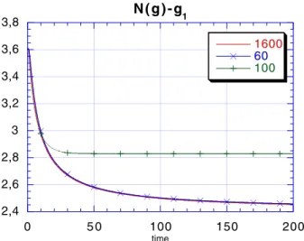
2,4 2,6 2,8 3 3,2 3,4 3,6 3,8 0 5 0 100 150 200 N ( g ) - g 1 1600 60 100 time
Figure 1: Density in case 1.
5
Numerical tests for the Kompaneets schemes
We will illustrate the scheme on the two following examples. The first one cor-responds to a Planck distribution multiplied by 3/2. In this case, concentration near origin occurs after few iterations since the initial density is greater than the critical one. On the second case, we consider a initial data with a lower density but we still observe a concentration when the initial density is close enough to 0, as expected after the analysis in [EHV] .
5.1
Relaxation of
αB
0with
α = 3/2
We plot the evolution in time of three macroscopic quantities, density for non zero energy, energy and entropy. The runs corresponds to the following three cases
• label ”1600” is a reference computation with 1600 points of discretizations and g0(0) = 0.
• label ”100” corresponds to 100 points using the same method and with g0(0) = 0.
• label ”60” denotes the same method but with only 60 points and with an initial data g0(0) += 0 but very small (10−12).
More precisely, in Fig1.1 we plot the quantity)
i≥1gih (the indices start at 1) i.e. the discrete version of,k0
0,65 0,7 0,75 0,8 0,85 0,9 0,95 1 0 5 0 100 150 200 N ( k g ) 1600 60 100 time
Figure 2: Energy in case 1.
-2,2 -2,15 -2,1 -2,05 -2 -1,95 0 5 0 100 150 200 Entropy 1600 60 100 time
remains smooth. It decays when concentration occurs. Fig. 2 (resp. 3) illustrates the evolution of the energy (resp. entropy). The differences of the three runs are in the number of discretization points and in the initial data (at zero energy). Indeed, as explained before (section 3.2.5) there are two ways to discretize the singularity. Either, g0(0) then, g0(t) = 0, ∀t > 0 and the distribution function converges to a generalized Bose-Einstein equilibrium (with µ < 0) that converges in a distributional sense toward the Planck distribution (B0) plus a dirac measure at k = 0 or g0(0) += 0 and the discretized distribution function converges for i ≥ 0 toward the Planck distribution, and the remaining density concentrates on k0= 0. The presented results show that it is much better to discretize with g0(0) += 0, in particular in terms of entropy (the entropy is lower with only 60 points and g0(0) += 0 than with 1600 points and g0(0) = 0, i.e. generalized Bose-Einstein equilibrium).
5.2
Initial gaussian distribution.
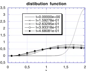
In this case, we consider an initial gaussian distribution with a sub-critical den-sity N < N0. In the Compton case (or QBE), the solution goes toward its Bose Einstein equilibrium. It has been proved in [EHV] that, for the Kompaneets equation, the solution may not be global in time provided that the initial density is close enough to the origin. Indeed, there is a balance between the Burgers term and the diffusion term : the Burgers part is a convective toward the origin that leads to concentration, whereas the diffusion spreads off the distribution that becomes smoother.
In Fig 1.4, we plot the distribution for different time when the initial data is a Gaussian centred at k = 2 with 3200 points of discretization. In this case, the diffusion dominates and the distribution function goes to its Bose-Einstein distribution (with ν > 0. In Fig 1.5, we plot the same quantities (distribution function versus k at different time) but with an gaussian initial data (same total density, centered at k = 1). In this case, the Burgers term is stronger and the distribution function becomes singular near origin after a finite time T∗. Clearly, the solution is no more valid for t > T∗but the simulation can be continued since the Kompaneets discretization can be interpreted as the discretization of QBE with a small parameter ε linked to the discretization step h (see section section 3.2.1) for which such a concentration is possible.
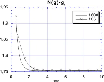
On Fig 1.6, we plot the evolution in time of the density for non zero energy and we observe the concentration at time T∗ : some part of the density goes into the zero energy part of the distribution function. On Fig 1.7 (resp. 1.8), we plot the energy (resp. entropy) versus time.
-0,5 0 0,5 1 1,5 2 2,5 3 3,5 0 0,5 1 1,5 2 distibution function t=0.00000e+00 t=1.59278e-01 t=2.63295e-01 t=3.93318e-01 t=4.68081e-01 k
Figure 4: Evolution of the distribution function in case 2, k = 2.
0 0,5 1 1,5 2 2,5 3 3,5 0 0,5 1 1,5 2 distribution function t=0.00000e+00 t=1.59278e-01 t=2.63295e-01 t=3.93318e-01 t=4.68081e-01 k
1,75 1,8 1,85 1,9 1,95 0 2 4 6 8 1 0 N ( g ) - g 1 1600 105 time
Figure 6: Density versus time in case 2 , k = 1.
0,9 0,92 0,94 0,96 0,98 1 1,02 0 2 4 6 8 1 0 N ( k g ) 1600 105 time Figure 7: energy -2,5 -2 -1,5 -1 -0,5 0 0,5 0 2 4 6 8 1 0 Entropy 1600 105 time Figure 8: entropy
6
Conclusions
The main improvements compared with the previous method investigated in [P] are
• This method does not require to construct a equilibrium state that usually required an iterative method (which is not always conservative).
• The semi-discretized system preserve all the properties : decay of entropy, conservation of density
• The semi-implicit scheme is unconditionally positive • Scheme 1 is of order 2 in k
Moreover, we are able to deal with condensation near the origin when the initial data has a density larger than the Planck one or is to close to the origin, both of these phenomena are illustrated by numerical results. There are two ways to describe this concentration at the discrete level : either g0(0) = 0 and then, this remains equal 0 at all time - in this case, the equilibrium state are generalized Bose-Einstein state with µ < 0 that converge in a distribution sense to the Planck distribution plus a Dirac at k = 0, see section 3.2.5 and appendix B - or g0(0) += 0 - in this case, the smooth part converges toward the Planck distribution and the remaining density concentrates on k = 0. The preliminary numerical results indicate that the second case is better and more precisely, that the first case is unstable : when the initial data at k = 0 is not equal zero, the scheme converges toward the second representation of the singularity.
Some questions remain to be attend in further works : • Is the semi-implicit scheme entropic ?
• How to construct a full implicit scheme (without iterative method) ? • Can we insure the same properties for general cross sections with the (QBE).
Appendix A : proof of Lemma 2.2
Proof. We begin by the first part of the lemma. It is then easy to check that it suffice to prove the result only in the case µ = 0, i.e. for B0.
For k ∈ [0, log+(α)] with log+(x) = max(0, log(x)), since the solution is non negative and
h(g, k) ≤ 1 ≤ α exp(−k) = αh(B0, k).
For k ∈] log(α), ∞[, consider any function G(x) such that G(x) ≥ 0 for x ≥ 0, 0 < G"(x) < ∞ for x ≥ 0 and G(x) = 0 for x ≤ 0. Then, define H
α(x, k) as Hα(x, k) = ! x x0 G" h(s, k) h(B0, k) − α # ds
for k ∈] log+(α), ∞[ with x0 the unique positive solution of h(x0, k) = αh(B0, k) (note that x0 = αk
2exp(−k)
1−α exp(−k) > 0) and Hα(x, k) = 0 for k ≤ log +(α). Set now E(t) = ! k≥0 Hα(g(k), k)dk.
It can be checked that by construction E(t) ≥ 0, E(t) is continuous and by the hypothesis E(0) = 0. Moreover, E(t) is C1 and we have
d dtE = ! k≥0 G" h(g, k) h(B0, k) − α# dg dtdk.
Now using the weakform (2.5) of the QBE, it is easy to see that, since G*h(Bh(g,k)0,k)−α+ is monotone increasing in the variable g for each k. Thus, using the inequality (x − y) (φ(x) − φ(x)) ≥ 0, for any monotone increasing function φ, d
dtE ≤ 0.
For the K equation, using the weak form (2.12), it is also clear that d
dtE ≤ 0. Thus, for both equation, E(t) = 0 for all time t, which is equivalent to h(Bh(g,k)0,k) ≤ α almost everywhere in k ∈] log+(α), ∞[.
For the proof of the second part of the lemma we proceed as for the first part. With the function G defined above, we set H as
H(x, k) = ! x x1 G" 1 − h(s, k h(B0, k) # ds, if g ≤ x1. and H(x, k) = 0 for g ≥ x1 and define
E(t) = !
k≥0
H(g, k)dk.
Proceeding as for the first part we obtain that E(t) is monotone decreasing, positive and E(0) = 0. Thus for any time E(t) = 0 that is h(g, k) ≥ h(B0, k)a.e. as we have claimed it.
Appendix B : proof of Proposition 3.3
Proof. As explained above α is a function of N and of h. Define N(α, h) as (for any h ≥ 0 and α ≥ −h)
N(α, h) =
! ∞
h
k2
exp(k + α) − 1dk.
The equation N(α, h) = N determines implicitly α as a function of N and h If N > N0, since N0 = N(0, 0), α(N, h) ∈ [−h, 0[ thus α → 0 as h → 0. Let φ a test function, we have
L(h) = ! ∞ 0 φ(k)(Mh(k)−B0(k))dk = ! ∞ h k2φ(k) exp(k + α(h)) − 1dk− ! ∞ 0 k2φ(k) exp(k) − 1dk.
We write φ(k) = φ(0) + kψ(k) where ψ is a C∞(0, ∞). We know that α(h) → 0. Thus, we have L(h) = ! ∞ h k2φ(0) " 1 exp(k + α(h)) − 1 − 1 exp(k) − 1 # dk + + ! ∞ h k3ψ(k) " 1 exp(k + α(h)) − 1 − 1 exp(k) − 1 # dk − ! h 0 k2φ(k) exp(k) − 1dk. The first term gives
! ∞ h k2 " 1 exp(k + α(h)) − 1 − 1 exp(k) − 1 # dk = N− ! ∞ h k2 exp(k) − 1dk → N−N 0.
- the second can be written as (1 − exp(α(h))
! ∞
h
k3ψ(k)dk
(exp(k + α(h)) − 1)(exp(k) − 1)dk → 0, and the third term goes to 0. Thus, we proved that
L(h) → (N − N0)φ(0). This is equivalent to the convergence of Bh
α toward B0+ (N − N0)δ0 in the dis-tribution sense.
Let us now consider the case N < N0. There exists β > 0 such that N(β, 0) = N. We want to prove that α(h) (N being fixed) goes to β as h → 0. The function α being decreasing with h and being positive for h small enough, one has 0 < α(h) < β. Moreover, α is continuous, then limh→0α(h) = α(0) = β. Then by dominated convergence theorem, we have that Bh
α tends to Bβ in L1(0, ∞) (and in the distributional sense).
Let us now prove the convergence of the entropy. One has H(g) = ! ∞ 0 " g log( g k2+ g) + k 2log( k2 k2+ g) + kg # dk. For the function Bh
α, one easily checks that Bh α k2+ Bh α = e−(k+α), k2 k2+ Bh α = 1 − e−(k+α). Then, using the expression of H and Bh
α, one obtains H(Bh α) = −α ! ∞ 0 Bh α+ ! ∞ h k2log (1 − exp −(k + α)) dk.
The first term is equal to −αN that goes to 0 because α → 0. Let us note gh(k) = log (1 − exp −(k + α)). We know that gh converges to g0 almost everywhere and is integrable on [0, ∞[. Note that ∀k > ε since α ≤ 0, (g0− gh)(k) ≥ 0.
(g0−gh)(k) = log " 1 − exp −(k) 1 − exp −(k + α) # ≤ exp(α)(exp(−α)−1) ! ∞ h k2dk exp −(k + α) − 1 using log(1 + h) ≤ h. This proves that
! ∞ h (g0− gh)(k)dk → 0. But, H(Bαh) − H(B0) = −αN + ! ∞ h (gh− g0)(k)dk − ! h 0 g0(k)dk.
The last term tends to 0 since g0 is integrable. This proves the convergence. In the second case N < N0 we know that α(h) is a decreasing function of h that converges toward β > 0 such that
! ∞
0
k2dk
exp(k + β) − 1 = N The proof given for N > N0 can be applied in this case.
Bibliography
[BP] Berman, A., Plemmons R.J., Nonnegative matrices in the mathemat-ical sciences. Classics in Applied Mathematics, 1994
[B] S. N. Bose, Plancks Gesetz und Lichtquantenhypothese, Z. Phys. 26 (1924), 178–181.
[BCF] Buet, Christophe, Cordier, St´ephane and Filbet, Francis, Com-parison of numerical schemes for Fokker-Planck-Landau equation. ESAIM Proc., vol 10, p. 161-181, (2001).
[BC] Buet, C. and Cordier, S., Numerical analysis of conservative and entropy schemes for the Fokker-Planck-Landau equation., SIAM J. Numer. Anal., vol 36, No 3, p. 953-973, (1998).
[BCDL] Buet, C.; Cordier, S.; Degond, P.; Lemou, M. Fast algorithms for numerical, conservative, and entropy approximations of the Fokker-Planck-Landau equation. J. Comput. Phys. 133, No.2, p. 310-322, (1997).
[CL] R.E. Caflisch, C.D. Levermore, Equilibrium for radiation in a homo-geneous plasma, Phys. Fluids 29, 748-752 (1986)
[CC] Chang J.S., Cooper G., A practical difference scheme for Fokker-Planck equations. J. Comput. Phys. 6, 1-16 (1970).
[C] G. Cooper, Compton Fokker-Planck equation for hot plasmas, Phys. Rev. D 3, 2312-2316 (1974)
[DV] L. Desvillettes, C. Villani, On the Spatially Homogeneous Landau Equation for Hard Potentials. Part I: Existence, Uniqueness and Smooth-ness, CPDE vol. 25, n. 1-2, (2000), pp. 179-259 and Part II: H–Theorem and Applications , CPDE, vol. 25, n. 1-2, (2000), pp. 261-298.
[EHV] M. Escobedo, M.A. Herrero, J.J.L. Velazquez, A nonlinear Fokker-Planck equation modeling the approach to thermal equilibrium in a homo-geneous plasma, Trans. Amer. Math. Soc. 350, 3837-3901 (1998)
[EM1] M. Escobedo, S. Mischler, Equation de Boltzmann quantique ho-mog`ene: existence et comportement asymptotique, Note au C. R. Acad. Sci. Paris 329 S´erie I, 593-598 (1999)
[EM2] M. Escobedo, S. Mischler: On a quantum Boltzmann equation for a gas of photons, J. Math.Pures Appl. 80, 5 (2001), pp. 471-515.
[EM3] M. Escobedo, S. Mischler, M.A. Valle, On Boltzmann equation for a gas of quantum (and relativistic) particles, work in preparation
[EMV] M. Escobedo, S. Mischler, J.J.L. Velazquez, Specified long time behavior for the Boltzmann-Compton equation, work in preparation [Ka] O. Kavian, Remarks on the Kompaneets Equation, a Simplified Model of the Fokker Planck equation, to appear in S´eminaire J.L. Lions - Coll`ege de France - s´erie rouge (Pitman-Longman-Wesley)
[K] A.S. Kompaneets, The establishment of thermal equilibrium between quanta and electrons, Soviet Physics JETP, (1957)
[Ku] Kullback, S. , On the convergence of discrimination information. IEEE Trans. Information Theory IT-14 1968 765–766
[LLPS] Larsen E.W., Levermore C.D., Pomraning G.C., Sanderson J.G. Discretization methods for one-dimensional Fokker-Planck operators. J. Comput. Phys. 61, 359-390 (1985)