HAL Id: hal-00753142
https://hal.inria.fr/hal-00753142
Submitted on 18 Nov 2012
HAL is a multi-disciplinary open access
archive for the deposit and dissemination of
sci-entific research documents, whether they are
pub-lished or not. The documents may come from
teaching and research institutions in France or
abroad, or from public or private research centers.
L’archive ouverte pluridisciplinaire HAL, est
destinée au dépôt et à la diffusion de documents
scientifiques de niveau recherche, publiés ou non,
émanant des établissements d’enseignement et de
recherche français ou étrangers, des laboratoires
publics ou privés.
A Comparative Study of Algorithms for Intra- and
Inter-subjects fMRI Decoding
Vincent Michel, Alexandre Gramfort, Evelyn Eger, Gaël Varoquaux, Bertrand
Thirion
To cite this version:
Vincent Michel, Alexandre Gramfort, Evelyn Eger, Gaël Varoquaux, Bertrand Thirion. A
Compar-ative Study of Algorithms for Intra- and Inter-subjects fMRI Decoding. MLINI - Machine Learning
and Interpretation in Neuroimaging - 2011, Dec 2011, Sierra Nevada, Spain. pp.1-8,
�10.1007/978-3-642-34713-9_1�. �hal-00753142�
A comparative study of algorithms for intra- and
inter-subjects fMRI decoding
Vincent Michel1, Alexandre Gramfort1, Evelyn Eger2, Ga¨el Varoquaux1, and
Bertrand Thirion1
1
Parietal team,INRIA Saclay-ˆIle-de-France / CEA, DSV, I2BM, Neurospin
2
INSERM U562 / CEA, DSV, I2BM, Neurospin
Abstract. Functional Magnetic Resonance Imaging (fMRI) provides an unique opportunity to study brain functional architecture, while being minimally invasive. Reverse inference, a.k.a. decoding, is a recent statis-tical analysis approach that has been used with success for deciphering activity patterns that are thought to fit the neuroscientific concept of population coding. Decoding relies on the selection of brain regions in which the observed activity is predictive of certain cognitive tasks. The accuracy of such a procedure is quantified by the prediction of the be-havioral variable of interest – the target. In this paper, we discuss the optimality of decoding methods in two different settings, namely intra-and inter-subject kind of decoding. While inter-subject prediction aims at finding predictive regions that are stable across subjects, it is plagued by the additional inter-subject variability (lack of voxel-to-voxel corre-spondence), so that the best suited prediction algorithms used in reverse inference may not be the same in both cases. We benchmark different prediction algorithms in both intra- and inter-subjects analysis, and we show that using spatial regularization improves reverse inference in the challenging context of inter-subject prediction. Moreover, we also study the different maps of weights, and show that methods with similar accu-racy may yield maps with very different spatial layout of the predictive regions.
1
Introduction
Reverse inference [1, 2], a.k.a. decoding, is an approach for mining fMRI data that uses pattern analysis in order to reveal the information produced by brain activations. The core of this approach is to consider fMRI data analysis as a pat-tern recognition problem, i.e. using a patpat-tern of voxels to predict a behavioral, perceptual or cognitive variable. In such studies, the accuracy of the prediction can be used to assess whether the pattern of voxels used in the predictive model actually encodes the information about the variable of interest. This approach has been used more frequently in intra-subject settings than in inter-subject anal-ysis. The main interest of inter-subject prediction is to find predictive regions that are stable across subjects, and thus obtain a population-level validation of cognitive hypothesis. The major bottleneck in inter-subject predictions is that such studies are plagued by the inter-subject variability (lack of voxel-to-voxel
correspondence) [3, 4]. Functional activity localization can vary across subjects due to differences in anatomical structure and in functional organization. As a result, it is challenging to find a common spatial layout of the cognitive sub-strate across different subjects. In this paper we compare different prediction algorithms in both intra- and inter-subjects settings, in order to investigate the properties required for good inter-subject prediction. We show that using spatial regularization improves the performances in the case of inter-subject studies, by gaining robustness against the spatial variability of the fMRI signal. We also compare the maps obtained by the different methods, and show variability in the spatial support of the predictive regions.
2
Methods
We briefly introduce the following predictive linear model, in regression settings y = X w + b, where y ∈ Rnrepresents the behavioral variable and (w, b) are the
parameters to be estimated on a training set. A vector w ∈ Rpcan be seen as an
image; p is the number of features (or voxels) and b ∈ R is called the intercept. The matrix X ∈ Rn×pis the design matrix. Each row is a p-dimensional sample,
i.e., an activation map related to the observation. The model performance is evaluated using ζ, the ratio of explained variance (or R2 coefficient), where
ζ(yt,ˆyt) = var(y
t
)−var(yt
−ˆyt
)
var(yt) . We now detail the different reference methods
that will be used in this study.
2.1 Non spatially-regularized methods
All the methods are used after an Anova-based feature selection, as this increases their performance. This selection is performed on the training set of each fold in an internal cross-validation loop, and the optimal number of voxels is selected within the range {50, 100, 250, 500}. This feature selection is performed for each method and for each training set separately. It yields different sets of features as the selection is done jointly with the regression within the cross-validation loop. Indeed, some methods such as Elastic Net can perform their own multivariate feature selection, but this step of univariate feature selection allows to reduce the number of features for the regression methods, thus decreasing the computational time.
In this paper, the implementation of Elastic net is based on coordinate descent [5], while SVR is based on LibSVM [6]. Methods are used from Python via the Scikit-learn open source package [7].
Support Vector Regression - SVR - The first prediction function used in reverse inference [2] has been Support Vector Machine (SVM) [8]. This ap-proach is widely used and has become the reference apap-proach for fMRI reverse inference. Its success comes from its wide availability and good performance on high-dimensional data. In this paper, we use SVR with a linear kernel. The C parameter is optimized by internal cross-validation in the range 10−3 to 101in
Elastic net regularization - Other approaches include built-in feature selec-tion: a generic formulation is given by Elastic net [9], which uses a combined ℓ1 (Lasso, parametrized by λ1) and ℓ2 (Ridge Regression, parametrized by λ2)
penalization. While setting many weights to zero, Elastic net, unlike Lasso, can extract more features than samples and correlated features. Elastic net is there-fore an attractive approach for reverse inference, as we expect to extract some groups of correlated features, while seeking for an interpretable model (i.e. few selected groups). We use a cross-validation procedure within the training set to optimize the parameters, with λ1 ∈ {0.2˜λ,0.1˜λ,0.05˜λ,0.01˜λ} (˜λ = kXTyk∞),
and λ2∈ {0.1, 0.5, 1., 10., 100.}.
Bayesian Ridge Regression - BRR - Bayesian Ridge regression is based on the following Gaussian assumptions p(y|X, w, α) = Qni=1N (yi|Xiw, α−1),
p(ǫ|α) = N (0, α−1I
n) (Gaussian noise), and p(w|λ) = N (w|0, λ−1Ip). This
Bayesian framework includes the explicit estimation of the α and λ parameters, through the direct maximization of the marginal likelihood. The price to pay is the non-convexity of the whole estimation procedure.
Automatic Relevance Determination - ARD - One can use a more strin-gent prior on w, known as ARD [10, 11], where we assume that the weights wiare
drawn from independent Gaussian distributions centered about zero and with a precision λi (λi6= λj if i 6= j): p(w|λ) = N (0, Λ−1) with Λ = diag {λ1, ..., λp} .
This choice of hyper-parameters yields very sparse models.
Multi-Class Sparse Bayesian Regression (MCBR) - MCBR - We also use the MCBR approach [12], which is an intermediate between BRR and ARD. MCBR consists in grouping the features into Q different classes, and regularizing these classes differently; as a consequence, it requires the estimation of fewer parameters than ARD and is far more adaptive than BRR. In this paper, we set K = 9, with weakly informative priors λ1,k= 10k−4, k∈ [1, .., K] and λ2,k=
10−2 , k ∈ [1, .., K], and α
1 = α2 = 1, following the work in [12]. MCBR can
be estimated using Gibbs sampling (Gibbs-MCBR) or Variational Bayes (VB-MCBR).
2.2 Spatially-regularized methods
Searchlight The searchlight [13] is a brain mapping approach, that yields the amount predictive information conveyed by the voxels in any sub-region about the target variable. This approach is used here for comparing the weights maps obtained by the predictive approaches. In this paper, we use spherical regions with a radius of two voxels, combined with an SVR function (C = 1).
Supervised clustering - SC The supervised clustering algorithm [14] is a procedure that creates parcels (i.e. spatially structured group of voxels), while
considering the target to be predicted as early as in the clustering procedure. It yields an adaptive segmentation into both large regions and fine-grained infor-mation, and can thus be considered as multi-scale. We used the SC with BRR, and we set ∆ = 75 (depth of exploration), following the work in [14].
Total Variation regularization - TV TV is defined as the ℓ1 norm of the image gradient, and has primarily been used for image denoising [15] as it pre-serves edges. The motivation for using TV for brain imaging [16] is that it promotes estimates of the weights with a block structure, therefore outlining the brain regions involved in the target behavioral variable. A particularly important property of this approach is its ability to create spatially coherent regions with similar weights, yielding simplified and informative sets of features. We use TV with a regularization parameter λ = 0.05, following the work in [16].
3
Experiments
We apply the different methods on a real fMRI dataset related to an exper-iment studying the representation of objects, as detailed in [17]. During this experiment, ten healthy volunteers viewed objects from one of two categories (each one of the two categories used in equal halves of subjects) with 4 differ-ent exemplars each shown in 3 differdiffer-ent sizes (yielding 12 differdiffer-ent experimdiffer-ental conditions), with 4 repetitions of each stimulus in each of the 6 sessions. We averaged data from the 4 repetitions, resulting in a total of n = 72 images by subject (one image of each stimulus by session). Functional images were acquired on a 3-T MR system with eight-channel head coil (Siemens Trio, Erlangen, Ger-many) as T2*-weighted echo-planar image (EPI) volumes. Twenty transverse slices were obtained with a repetition time of 2 s (echo time, 30 ms; flip angle, 70◦; 2×2×2-mm voxels; 0.5-mm gap). Realignment, normalization to MNI space,
and General Linear Model (GLM) fit were performed with the SPM5 software http://www.fil.ion.ucl.ac.uk/spm/software/spm5. In the GLM, the effect of each of the 12 stimuli convolved with a standard hemodynamic response function was modeled separately, while accounting for serial autocorrelation with an AR(1) model and removing low-frequency drift terms by a high-pass filter with a cut-off of 128 s. In the present work we used the resulting session-wise parameter estimate images. All the analysis are performed on the whole brain volume. Intra-subject experiment The four different shapes of objects (from either cat-egory) were pulled for each of the three sizes, and we are interested in finding discriminative information between sizes. Each subject is evaluated indepen-dently, in a leave-one-condition-out cross-validation (i.e., leave-6-images-out). The parameters of the different methods are optimized with a nested leave-one-condition-out cross-validation within the training set.
Inter-subject experiment The inter-subject analysis relies on subject-specific fixed-effects activations, i.e. for each condition, the 6 activation maps corre-sponding to the 6 sessions are averaged together. This yields a total of 12 images
per subject, one for each experimental condition. We evaluate the performance of the method by cross-validation (leave-one-subject-out). The parameters of the different methods are optimized with a nested leave-one-subject-out cross-validation within the training set. Spatial correspondence of images within be-tween subjects was assumed after realignment and normalization to the MNI space had been carried out, based on the available anatomical image of each subject.
4
Results
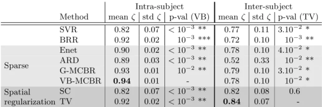
The results obtained in both intra-subject and inter-subject experiments are given Table. 1 (p-values are computed using a paired t-test).
Intra-subject Inter-subject Method mean ζ std ζ p-val (VB) mean ζ std ζ p-val (TV) SVR 0.82 0.07 <10−3 ** 0.77 0.11 3.10−2 * BRR 0.92 0.02 10−3 *** 0.72 0.10 10−3 ** Enet 0.90 0.02 <10−3 ** 0.78 0.10 4.10−2 * ARD 0.89 0.03 <10−3 ** 0.52 0.33 10−2 ** G-MCBR 0.93 0.01 10−2 ** 0.79 0.10 3.10−2 * Sparse VB-MCBR 0.94 0.01 - 0.78 0.10 10−2 * SC 0.82 0.07 <10−3 ** 0.82 0.08 0.6 Spatial regularization TV 0.92 0.02 <10−3 ** 0.84 0.07
-Table 1. Prediction performance: explained variance ζ for different methods. Sparse methods are in light gray, and spatially-regularized methods in dark gray.
Intra-subject analysis The two sparsity-adaptive approaches VB-MCBR and Gibbs-MCBR outperform the alternative methods, yielding an average explained variance of 0.94 and 0.93 across the subjects. Moreover, their results are more stable across subjects. The SC algorithm and SVR perform poorly.
Inter-subject analysis In this study, TV regression outperforms the non spa-tially regularized methods, yielding an average explained variance of 0.84, and also more stable predictions. SC also performs well, with an average explained variance of 0.82. ARD, which yields the sparsest model, performs poorly.
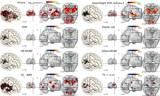
Inter-subject analysis - Interpretability of the resulting maps In the case of a linear prediction function, it is easy to look at the voxels weights used in the model. Indeed, these maps can be used to study some large-scale characteristics of the encoding of the cognitive information in brain regions. In general, one might expect the spatial layout of neural activity to be sparse and spatially structured in the sense that non-zero weights are grouped into connected clusters. Weighted maps showing such characteristics will be called interpretable, as they reflect our hypothesis on the spatial layout of the neural activity. We give Fig. 1 the images obtained with the different methods. From
Fig. 1. Maps obtained for different methods studied, in the inter-subject analysis. First row: the two brain mapping approaches Anova (left) and Searchlight (right) found similar regions. Second row: SVR (left) and Elastic net (right) retrieve part of the spatial structure of the predictive regions, similarly to VB-MCBR (third row, left) and Gibbs-MCBR (third row, right). Fourth row: SC and TV create identifiable clusters.
a neuroscientific point of view, the regions are concentrated in the early visual cortex. Indeed, the processings of visual information about sizes are performed in early occipital cortex, with some extent in more parietal regions [17].
We can see that the SC method creates identifiable clusters, yielding a map similar to the Searchlight procedure, but that it also retrieves additional clusters. TV regression also yields weight maps very similar to the maps obtained by a classical brain mapping approach (such as Anova or Searchlight) but more sparse. We can see that SC and TV benefits from the power of a predictive framework similarly to SVR and Elastic net, while providing brain maps similar to classical SPMs. This confirm the results obtained in terms of prediction accuracy, that spatial regularization is a good way to tackle the spatial variability problem in inter-subjects studies [4, 3]. On the contrary, voxel-based methods suffer from the inter-subject spatial variability, and do not yield interpretable maps, even when they achieve high prediction accuracy (e.g. Gibbs-MCBR). We can notice that Gibbs-MCBR, VB-MCBR and SVR yield similar maps, that retrieve a part of the spatial structure obtained in brain mapping approaches. However, Elastic net, while achieving high prediction accuracy, yields very sparse map that is difficult to interpret to retrieve the spatial support of the neural activity.
5
Discussion
Bayesian versus classical discriminative approaches The methods presented can be roughly classified in two groups: Bayesian approaches (e.g. BRR, ARD,
Gibbs-MCBR and VB-Gibbs-MCBR) and classical approaches (e.g. Elastic net, SVC or To-tal Variation framework). In term of prediction accuracy, the two types of ap-proaches performed similarly, with a slight advantage of the Bayesian methods in the intra-subject analysis. An explanation is that such approaches can more finely estimate the regularization parameter which is not restricted to a pre-defined grid. A finer grid would be possible but would require more computa-tion. In the inter-subject analysis, classical approaches perform slightly better, because the parameter tuning by internal cross-validation makes them less prone to overfit a particular training subset of subjects.
Sparse versus non-sparse discriminative approaches It is interesting to compare the performance of BRR, ARD and MCBR as they perform a Bayesian regular-ization with different degree of sparsity. In intra-subject, MCBR performs better than BRR and ARD, as the number of classes may be used to adapt the sparsity between the two extremal cases of BRR (no sparsity), and ARD (high sparsity). In inter-subject, MCBR still performs better than BRR and ARD, but there is an increase in the difference of accuracy between the different methods. Thus, it seems promising to develop methods that are able to adapt their sparsity to the specificity of the dataset, yielding a high regularization (intra-subject), and a less drastic regularization (inter-subject).
Impact of spatial regularization We can see a clear dissociation between intra-subject and inter-intra-subject analyzes. This can be explained by the different intrin-sic resolution of spatial information present in intra and inter-subject settings. Indeed, prediction can rely on relatively sparse and fine-grained patterns at the single subject level. On the opposite, in inter-subject settings, it must be robust to misalignments. Such robustness is obtained through spatial regularization, as in supervised clustering and total variation penalization.
Interpretability of the resulting maps We have seen that spatially regularized methods yield more interpretable maps that other voxel-based methods. More-over, compared to a state of the art approach for fine-grained decoding, namely the searchlight, SC and TV yield similar maps, but additionally, take into ac-count non-local information and also have the advantages of a predictive frame-work (e.g. a prediction score corresponding to whole brain). A joint comparison between the prediction accuracies and the resulting maps also shown that it is difficult to choose a method close to a potential ground truth. A good prediction accuracy and interpretable map do not always come together.
Conclusion In this paper, we compare different prediction algorithms in both intra- and inter-subject analysis. We show that using spatial information within voxel-based analysis with Total Variation regularization, or by creating interme-diate structure as parcels, makes it possible to deal with spatial variability, and yields accurate and interpretable results for reverse inference. We also find that Bayesian approaches, by tuning more precisely the level of sparsity, work well for
intra-subject analysis. They might however be trapped into local minima more easily, and did not perform very well in inter-subject experiments.
References
1. S. Dehaene, G. Le Clec’H, L. Cohen, J.-B. Poline, P.-F. van de Moortele, and D. Le Bihan, “Inferring behavior from functional brain images,” Nature Neuro-science, vol. 1, p. 549, 1998.
2. D. D. Cox and R. L. Savoy, “Functional magnetic resonance imaging (fMRI) ”brain reading”: detecting and classifying distributed patterns of fMRI activity in human visual cortex.” Neuroimage, vol. 19, pp. 261–270, 2003.
3. A. Tucholka, “Prise en compte de l’anatomie c´er´ebrale individuelle dans les ´etudes d’IRM fonctionnelle,” Ph.D. dissertation, Universit´e Paris-Sud, 2010.
4. A. M. Tahmasebi, “Quantification of Inter-subject Variability in Human Brain and Its Impact on Analysis of fMRI Data,” Ph.D. dissertation, Queen’s University, 2010.
5. J. Friedman, T. Hastie, and R. Tibshirani, “Regularization paths for generalized linear models via coordinate descent,” Journal of Statistical Software, vol. 33, no. 1, 2010.
6. C.-C. Chang and C.-J. Lin, LIBSVM: a library for support vector machines, 2001, software available at http://www.csie.ntu.edu.tw/ cjlin/libsvm.
7. F. Pedregosa, G. Varoquaux, A. Gramfort, V. Michel, B. Thirion, O. Grisel, M. Blondel, P. Prettenhofer, R. Weiss, V. Dubourg, J. Vanderplas, A. Passos, D. Cournapeau, M. Brucher, M. Perrot, and E. Duchesnay, “Scikit-learn: Machine Learning in Python ,” Journal of Machine Learning Research, vol. 12, pp. 2825– 2830, 2011.
8. C. Cortes and V. Vapnik, “Support vector networks,” in Machine Learning, vol. 20, 1995, p. 273.
9. H. Zou and T. Hastie, “Regularization and variable selection via the elastic net,” J. Roy. Stat. Soc. B, vol. 67, p. 301, 2005.
10. D. J. C. MacKay, “Bayesian interpolation,” Neural Comput., vol. 4, no. 3, pp. 415–447, 1992.
11. R. M. Neal, Bayesian Learning for Neural Networks (Lecture Notes in Statistics), 1st ed. Springer, 1996.
12. V. Michel, E. Eger, C. Keribin, and B. Thirion, “Multiclass Sparse Bayesian Re-gression for fMRI-Based Prediction,” International Journal of Biomedical Imaging, vol. 2011, Apr. 2011.
13. N. Kriegeskorte, R. Goebel, and P. Bandettini, “Information-based functional brain mapping.” Proceedings of the National Academy of Sciences of the United States of America, vol. 103, no. 10, pp. 3863–3868, March 2006.
14. V. Michel, A. Gramfort, G. Varoquaux, E. Eger, C. Keribin, and B. Thirion, “A supervised clustering approach for fMRI-based inference of brain states,” Pattern Recognition, Apr. 2011.
15. L. Rudin, S. Osher, and E. Fatemi, “Nonlinear total variation based noise removal algorithms,” Physica D, Jan 1992.
16. V. Michel, A. Gramfort, G. Varoquaux, E. Eger, and B. Thirion, “Total varia-tion regularizavaria-tion for fMRI-based predicvaria-tion of behaviour.” IEEE Transacvaria-tions on Medical Imaging, vol. 30, no. 7, pp. 1328 – 1340, 2011.
17. E. Eger, C. Kell, and A. Kleinschmidt, “Graded size sensitivity of object exem-plar evoked activity patterns in human loc subregions,” J. Neurophysiol., vol. 100(4):2038-47, 2008.