A multi-model analysis of risk of ecosystem shifts under climate change

HAL Id: hal-02930052

https://hal.archives-ouvertes.fr/hal-02930052

Submitted on 8 Sep 2020

HAL is a multi-disciplinary open access

archive for the deposit and dissemination of

sci-entific research documents, whether they are

pub-lished or not. The documents may come from

teaching and research institutions in France or

abroad, or from public or private research centers.

L’archive ouverte pluridisciplinaire HAL, est

destinée au dépôt et à la diffusion de documents

scientifiques de niveau recherche, publiés ou non,

émanant des établissements d’enseignement et de

recherche français ou étrangers, des laboratoires

publics ou privés.

A multi-model analysis of risk of ecosystem shifts under

climate change

Lila Warszawski, Andrew Friend, Sebastian Ostberg, Katja Frieler, Wolfgang

Lucht, Sibyll Schaphoff, David Beerling, Patricia Cadule, Philippe Ciais,

Douglas Clark, et al.

To cite this version:

Lila Warszawski, Andrew Friend, Sebastian Ostberg, Katja Frieler, Wolfgang Lucht, et al.. A

multi-model analysis of risk of ecosystem shifts under climate change. Environmental Research Letters, IOP

Publishing, 2013, 8 (4), pp.044018. �10.1088/1748-9326/8/4/044018�. �hal-02930052�

Environmental Research Letters

LETTER • OPEN ACCESS

A multi-model analysis of risk of ecosystem shifts

under climate change

To cite this article: Lila Warszawski et al 2013 Environ. Res. Lett. 8 044018

View the article online for updates and enhancements.

Related content

Risk of severe climate change impact on the terrestrial biosphere

-Asynchronous exposure to global warming: freshwater resources and terrestrial ecosystems

-Impact of climate change on renewable groundwater resources: assessing the benefits of avoided greenhouse gas emissions using selected CMIP5 climate projections

-Recent citations

Quantitative assessment of fire and vegetation properties in simulations with fire-enabled vegetation models from the Fire Model Intercomparison Project

Stijn Hantson et al

-Relieved drought in China under a low emission pathway to 1.5°C global warming

Xu Yue et al

-The overlooked soil carbon under large, old trees

Christopher Dean et al

-IOP PUBLISHING ENVIRONMENTALRESEARCHLETTERS

Environ. Res. Lett. 8 (2013) 044018 (10pp) doi:10.1088/1748-9326/8/4/044018

A multi-model analysis of risk of

ecosystem shifts under climate change

Lila Warszawski

, Andrew Friend

, Sebastian Ostberg

, Katja Frieler

,

Wolfgang Lucht

, Sibyll Schaphoff

, David Beerling

, Patricia Cadule

,

Philippe Ciais

, Douglas B Clark

, Ron Kahana

, Akihiko Ito

,

Rozenn Keribin

, Axel Kleidon

, Mark Lomas

, Kazuya Nishina

,

Ryan Pavlick

, Tim Tito Rademacher

, Matthias Buechner

,

Franziska Piontek

, Jacob Schewe

, Olivia Serdeczny

and

Hans Joachim Schellnhuber

1_{Potsdam Institute for Climate Impact Research, D-14412 Potsdam, Germany} 2_{Department of Geography, University of Cambridge, Cambridge, UK} 3_{Department of Animal and Plant Sciences, University of Sheffield, UK} 4_{Laboratoire des Sciences du Climat et de l’Environment, Gif sur Yvette, France} 5_{Centre for Ecology and Hydrology, Wallingford OX10 8BB, UK}

6_{Met Office Hadley Centre, Exeter EX1 3PB, UK}

7_{Center for Global Environmental Research, National Institute for Environmental Studies, Japan} 8_{Max-Planck-Institut fuer Biogeochemie, PO Box 10 01 64, D-07701 Jena, Germany}

9_{Santa Fe Institue, Santa Fe, NM 87501, USA}

E-mail:lila.warszawski@pik-potsdam.de Received 24 June 2013

Accepted for publication 3 October 2013 Published 28 October 2013

Online atstacks.iop.org/ERL/8/044018

Abstract

Climate change may pose a high risk of change to Earth’s ecosystems: shifting climatic boundaries may induce changes in the biogeochemical functioning and structures of ecosystems that render it difficult for endemic plant and animal species to survive in their current habitats. Here we aggregate changes in the biogeochemical ecosystem state as a proxy for the risk of these shifts at different levels of global warming. Estimates are based on simulations from seven global vegetation models (GVMs) driven by future climate scenarios, allowing for a quantification of the related uncertainties. 5–19% of the naturally vegetated land surface is projected to be at risk of severe ecosystem change at 2◦C of global warming (1GMT) above 1980–2010 levels. However, there is limited agreement across the models about which geographical regions face the highest risk of change. The extent of regions at risk of severe ecosystem change is projected to rise with1GMT, approximately doubling between 1GMT = 2 and 3◦C, and reaching a median value of 35% of the naturally vegetated land surface for1GMT = 4◦C. The regions projected to face the highest risk of severe ecosystem changes above1GMT = 4◦C or earlier include the tundra and shrublands of the Tibetan Plateau, grasslands of eastern India, the boreal forests of northern Canada and Russia, the savanna region in the Horn of Africa, and the Amazon rainforest.

Keywords: climate change, ecosystem change, global vegetation

S Online supplementary data available fromstacks.iop.org/ERL/8/044018/mmedia

Climate change is likely to alter the biogeochemical functioning and structure of ecosystems, and therefore to

Content from this work may be used under the terms of theCreative Commons Attribution 3.0 licence. Any further distribution of this work must maintain attribution to the author(s) and the title of the work, journal citation and DOI.

affect the ability of plant and animal species to prosper in their current habitats [1]. Even before changes in the ecosystem are observed, the global terrestrial biosphere can be committed to long-term change [2], with potentially severe impacts on the complex interactions in trophic chains (e.g. between plant and animal species) [3] and on the ecosystems services provided

1

to societies [4]. Furthermore, greenhouse gas emissions can feed back on the climate [5] through shifts in productivity and decomposition [6].

Until now, attempts to study the impacts of climate change on these highly networked complex systems have taken two broad paths: (1) top-down approaches that utilize global vegetation models (GVMs) to assess the changes in large-scale biogeochemical variables such as net primary product (NPP) or vegetation carbon (Cveg), without explicitly modelling the impacts on the ecosystem as a whole, including complex interactions between plants, animals and disturbances; or (2) bottom-up studies of individual species or habitats [7,8], with necessarily limited coverage. Whilst comprehensive efforts to intercompare GVMs have provided a detailed picture of the spread in projections of key biogeochemical variables [9–12], studies that attempt to interpret these results in terms of impacts on the whole ecosystem have thus far been limited to single-model studies [13,14].

A multi-model study of climate change impacts on ecosystem functioning at the global scale requires an high level of coordination between modelling groups. In addition, a robust methodology is required to measure the relevance of biogeochemical changes for the complex interactions and dependences that characterize ecosystems. In this study we take a first step towards filling this gap. We assume that changes in the fundamental biogeochemical properties, which GVMs are well suited to simulate, can serve as proxies for the risk of more general shifts in these ecosystems. We argue that such shifts in the fundamental biogeochemistry are likely to imply transformations in the underlying system characteristics, such as species composition [15], and relationships between plants, herbivores and pollinators [3, 16,17]. For example, if the productivity of a land area increases or decreases, the composition of species it carries will be affected; similarly, prolonged drought or increased rainfall in an area will cause changes to trophic chains.

Some ecosystem changes induced by climate change could indeed be regarded as positive, including greater productivity through longer growing seasons, increases in nutrient richness, CO2 fertilization and migration into

previously poorly vegetated regions [18–21, 46]. Other changes could be regarded as detrimental, for example, reduced vegetation growth, increased limitations from decreasing soil moisture, increased occurrence of fires, or increased mortality of saplings. Whether the change is in the direction of more biogeochemical activity or less, it poses a risk of restructuring. We therefore do not subscribe to the common assumption that ‘more growth is better’ from the perspective of risk to currently existing ecosystems in their present locations.

Building on significant efforts in the past to compare the output from global biogeochemical models [12, 11, 10,9], we investigate biogeochemical and structural shifts simulated by seven GVMs, driven by the latest climate projections from multiple global climate models (GCMs) based on the representative concentration pathways (RCPs [22]). The simulations were performed as part of the Inter-Sectoral

Impact Model Intercomparison Project (ISI-MIP), which offers a consistent, cross-sectoral framework for the study of uncertainties in climate change impacts at different levels of global warming [23]. The project framework also allows for comparison and aggregation of impacts across sectors [24, 47], which are essential to understanding the impact of changing land-use patterns on natural ecosystems, and the competing interests of climate mitigation and food security [48].

1. Methods

1.1. The ecosystem shift proxy

GVMs are developed to simulate changes in biomass, carbon turnover, water flows and ecophysiological functional strategies (woody or non-woody, evergreen or deciduous, needleleaf or broadleaf etc) on a coarse scale. While changes in these stocks and fluxes are interesting in themselves, they do not directly reveal the risk of shifts in ecosystems under pressure from climate change. Ecosystems are characterized by complex networks of interactions between species, communities and their local niches. However, here we suggest using changes in the biogeochemical state of the vegetated land surface, as simulated by GVMs, as a proxy for risk of such change.

Following [15], we argue that any of the following effects are indicative of risk that ecosystem structures will be affected: change in functional strategies of the vegetation present (1V); relative, changes in local biogeochemical carbon and water stocks and fluxes (c); absolute, local change in biogeochemical stocks and fluxes with respect to globally averaged changes in stocks and fluxes (g); changes in the relative (to one another) magnitude of key biogeochemical exchange fluxes (b); or change in interannual variability of biogeochemical stocks and fluxes (S(x, σx)). The variability

term S(x, σx) is a normalized sigmoid function of the ratio

of the respective components to their standard deviation in the reference period. We use the aggregate of these effects, based on the biogeochemical quantities listed in table S3 (where ‘S’ refers to the supplementary material, available atstacks.iop.org/ERL/8/044018/mmedia), as a proxy for the risk of ecosystem shift, 0 [15]. The multiple dimensions are first normalized using a sigmoid function, and then combined according to

0 = [1V + cS(c, σc) + gS(g, σg) + bS(b, σb)]/4. (1)

Each of the components c, b and g is constructed by first considering a set of biogeochemical fluxes and stocks, which are combined into a state vector for each grid cell, at each point in time, and then comparing the state vector for the same grid cell at a given time with that of a reference period. In the case that a GVM does not model changes in vegetation composition, the vegetation composition change component of the metric (1V) is not included in the calculation of 0, resulting in an increased weighting of the other three components (c, b and g). A comprehensive description of the proxy can be found in [15].

Environ. Res. Lett. 8 (2013) 044018 L Warszawski et al

Our correlation of0 to risk of ecosystem change makes use of a space-for-time evaluation (i.e. using the difference between contemporaneous, but geographically separate states as a substitute for different points in time for the same location; see figure S1, available at stacks.iop.org/ERL/8/ 044018/mmedia). In the absence of both a well-founded theory of global-scale ecosystem changes under climate change, and a sufficient density and duration of instrumented test sites, space-for-time can give an indication of the degree of difference between ecosystem states implied by a given value of 0 [25]. We do not attempt to correlate 0 fully to risk of ecosystem change, but consider two thresholds for moderate and severe risk (0 = 0.1 and 0 = 0.3 respectively), chosen in view of the space-for-time analysis.

Comparison of two identical vegetation states produces 0 = 0, whereas a replacement of a biome by a completely different biome produces a Gamma of nearly 1 (e.g. 0 = 0.98 for a change from rainforest to semi-desert) [14]. Analysis shows that when global vegetation modelled by a GVM (here, LPJmL) is mapped into 16 major biomes, the difference between any two of these biomes is never smaller than about 0 = 0.1 [14], which is the value characterizing the difference between closely related, but different biomes, e.g. the difference between a temperate coniferous and a mixed forest. Hence, we designate0 = 0.1 as a substantial, but still moderate risk of shifts in ecosystem properties. Most between-biome differences are larger, with 0 = 0.3 characterizing, for example, the difference between a boreal evergreen forest and a temperate broadleaved deciduous forest (0 = 0.32), or a warm wood- and shrubland and a tropical seasonal forest (0 = 0.31). Since these biomes are substantially different, we designate changes of 0 > 0.3 as severe risk of ecosystem change. All other between-biome differences studied produce larger 0 [14]. For example, between a temperate grassland and Arctic tundra 0 = 0.57; between warm, woody savannah and a tropical rainforest 0 = 0.51; and between temperate and tropical vegetation 0 > 0.5. The table in figure S1 provides a comprehensive listing of0 values between different biomes and is based on calculations performed using the LPJmL model [14]. It should be noted that a number of factors may combine to produce a particular value of0; the examples given should be used as an illustrative guide only.

In order to calculate0 for each year, we calculate changes to the quantities listed in table S2 (available at stacks.iop. org/ERL/8/044018/mmedia) by comparing the running mean over a 30-year period centred on the year of interest and the average for the period 1980–2009, which is taken to be the baseline state of the ecosystem. The 30-year window ensures that year-to-year variability does not dominate the signal, favouring long-term shifts in the basic ecosystem properties. In addition, it allows for the required quantification of changes in the variability of the considered variables. Simulations were performed for the time frame 1980–2100. Where a contributing variable of 0 was not supplied by a model (see table S3), it was left out of the calculation. Where no dynamic vegetation composition was modelled, this component was not included in the calculation and the

other components (carbon and water stocks and fluxes) were scaled up accordingly (i.e. in equation (1),1V = 0 and the factor in the denominator is 3). The risk of ecosystem changes is presented at different levels of global mean temperature change (1GMT, compared to 1980–2009 levels, which are in turn approximately 0.7◦C above pre-industrial levels), thus contributing to the discussion about targets for limiting climate change.

1.2. Model simulations

This study reports results from seven GVMs, forced by the bias-corrected ISI-MIP climate data set [23] on a 0.5◦ × 0.5◦ grid (JeDi and JULES were simulated on a 1.25◦×1.85◦grid) for four RCPs, with and without variable atmospheric CO2 concentration. The bias correction method

maintained the climate sensitivities of the GCMs (absolute change in monthly mean temperature and relative change in precipitation and other climate variables), whilst adjusting the absolute mean monthly climate variables to statistically match a historical data set. The method also corrects the daily variability of all climate variables to statistically match the observational data set. A detailed description of the bias correction method can be found in [26].

Each GVM performed a spin-up separately for each GCM, with the aim of bringing carbon and water pools into equilibrium for 1950 climate conditions. This spin-up was performed by recycling de-trended climate fields simulated by each GCM over the period 1950–1980 (JULES performed a single spin-up using HadGEM2-ES data). The length of the spin-up was determined individually according to the needs of each model. A CO2concentration of 280 ppm was adopted for

the period until the year 1765. From 1765 CO2concentration

was increased according to historical data until 2006 [27]. The atmospheric CO2concentration for 2006–2100 is prescribed

by the four representative concentration pathways ([22] RCP 2.6, RCP 4.5, RCP 6.0 and RCP 8.5) used to drive the GCMs. Table S3 gives details of the model runs performed by each GVM in combination with the GCMs, as well as1GMT for the period 2070–2099 compared to the 1980–2009 for each climate scenario. Further description of the climate data set can be found in [23].

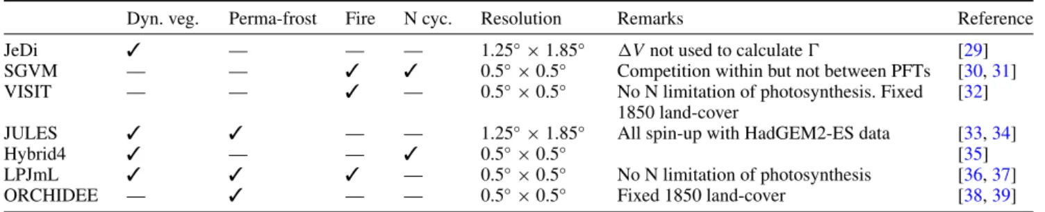
The GVMs and their main characteristics are summarized in table 1. The 0 proxy was calculated using all available variables from each model. Four of these models (LPJmL, Hybrid, JeDi and JULES) simulate the changing vegetation composition due to changing climate and atmospheric conditions, albeit with unique classification of plant types into clusters (see the supplementary material for a full listing, available atstacks.iop.org/ERL/8/044018/mmedia). For JeDi, the vegetation changes, denoted 1V, were not used to calculate 0, since the large number of growth strategies considered were not easily categorized as plant functional types, as required by 0. For the three models that provided dynamic vegetation composition (see table1for more details), 0 values were additionally calculated ignoring the 1V component (results shown in the supplementary material), in

Figure 1. The ecosystem component that individually results in the largest0 value according to the multi-model median. The blue, red and orange colours denote the dominance of the water, carbon flux and carbon stocks components of0 respectively. The intensity of the colour indicates the magnitude of the median of the dominant component. On 41% of the global naturally vegetated land surface carbon fluxes are the dominant component of0. Grey cells have <2.5% vegetation cover according to the GVMs, and white cells have <50% natural vegetation cover. Only the RCP 8.5 scenario for the HadGEM2-ES climate data for the year 2084 (2070–2099) is used here.

Table 1. Basic properties of participating ecosystem models.

Dyn. veg. Perma-frost Fire N cyc. Resolution Remarks Reference

JeDi 3 — — — 1.25◦

×1.85◦ _{1V not used to calculate 0}

[29]

SGVM — — 3 3 0.5◦_×

0.5◦

Competition within but not between PFTs [30,31]

VISIT — — 3 — 0.5◦_×

0.5◦

No N limitation of photosynthesis. Fixed 1850 land-cover

[32]

JULES 3 3 — — 1.25◦_×

1.85◦

All spin-up with HadGEM2-ES data [33,34]

Hybrid4 3 — — 3 0.5◦_× 0.5◦ [35] LPJmL 3 3 3 — 0.5◦_× 0.5◦ No N limitation of photosynthesis [36,37] ORCHIDEE — 3 — — 0.5◦_× 0.5◦ Fixed 1850 land-cover [38,39]

order to limit the inconsistency in comparing these two classes of models.

In contrast to the coupled climate–land-surface modelling intercomparison as part of CMIP5, in this exercise the entire global surface was assumed to be covered by natural vegetation only (i.e. no anthropogenic land-cover), resulting in output of only climate driven rather than land-use-change-driven vegetation composition and biogeochemical changes. In this way we separate the pure climate impact from the extensive impacts of changing human agricultural practices and urbanization and focus on the vulnerability of natural ecosystems. For the two models where agricultural pastures was part of the default setup (ORCHIDEE and VISIT), results for the naturally vegetated portion of each cell were scaled up to ‘fill’ the cell. For display purposes, cells with<50% natural vegetation cover (based on the MIRCA 2000 data set of irrigated and rainfed crop areas [28]) are not shown on the world maps (coloured white). However, for the aggregation of the total land surface at risk of ecosystem change, all grid cells with >2.5% actual vegetation cover according to the GVMs are considered and weighted by the fractional area of natural vegetation. For grid cells where actual vegetation cover<2.5%, no 0 is calculated (coloured grey in the world

maps) and the cells are not included in the aggregation calculations.

2. Results and discussion

2.1. Drivers of change

We quantify the risk of ecosystem change using the ecosystem shift proxy 0 described in [15]. In order to understand the drivers of the risk of ecosystem change, we first consider the relative contribution of changes to carbon stocks, carbon fluxes, water fluxes and vegetation composition changes (where available). This is done by calculating 0 as given in equation (1) for each GVM only for the chosen biogeochemical or vegetation properties. An example of the results are shown in figure 1, where the colour denotes the dominant component of 0 in 2084 for the median of the ecosystem-model ensemble for all RCP 8.5 GCM runs, and the intensity of the colour denotes the magnitude of that component (see also figures S13–S15, available at

stacks.iop.org/ERL/8/044018/mmedia). It should be noted, that these results do not represent the output of any one GVM, and that results across the GVMs vary both in

Environ. Res. Lett. 8 (2013) 044018 L Warszawski et al

Figure 2. Fraction of global natural vegetation (including managed forests) at risk of ecosystem change as a function of global mean temperature (left panels) and time (right panels) for the JeDi (left) and JULES (right) dynamic global vegetation model driven by the HadGEM2-ES global climate model. Results are shown for small (0 ≥ 0.1, circles) and severe (0 ≥ 0.3, diamonds) shifts. The colours represent the different RCPs used to drive the climate model. Good agreement of results at different levels of global warming demonstrate that results are independent of the emissions scenario. Similar plots for all ecosystem models and GCMs can be found in figure S8 (available atstacks.iop.org/ERL/8/044018/mmedia).

magnitude and spatial distribution. In most cases, changes to carbon fluxes between ecosystem and atmosphere (red colours in figure1) mainly drive the risk of ecosystem change, which arises from the climate sensitivity of photosynthesis, respiration and plant water-use efficiency to atmospheric CO2

concentrations increases. Steady increases with 1GMT in net primary production across all models except Hybrid, and total vegetation carbon across all models, is driven largely by CO2 fertilization of photosynthesis [46]. This is confirmed

by the reduced risk of ecosystem shift when atmospheric CO2levels are held constant at present-day levels (see figures

S2–S4, available at stacks.iop.org/ERL/8/044018/mmedia). This difference is more pronounced at low temperatures (e.g. LPJmL projects 5% natural vegetation at risk of severe ecosystem change with fixed, present-day CO2 compared to

16% with changing CO2 concentration at 1GMT = 2◦C)

compared to high temperatures (27–32% in both cases for LPJmL at 1GMT = 4◦C). The Amazon is an exception, where changes to water fluxes and carbon stores also play a prominent role in most ecosystem models (see figures S13–S15). For ORCHIDEE changes in water fluxes dominate in the far northern latitudes and for both ORCHIDEE and VISIT, changes in water fluxes also dominate the region in and around the Democratic Republic of the Congo.

No cells are dominated by vegetation change (1V, green) since four of the seven GVMs considered do not include dynamic vegetation composition changes. However, vegetation changes dominate 0 for some regions of the northern Boreal forests according to the three models with dynamic GVMs. Even when only these three models with dynamic vegetation are considered, only 4% of the land surface is dominated by vegetation changes (see figure S14), most notably due to shifts in the Boreal treeline northwards in Canada and Russia, greening in the Sahel, and transitions between grass and shrub biomes in western Russia and eastern India. The relatively small contribution of1V to the overall

value of 0 is further confirmed by the 15% reduction in land surface at risk of severe change when the vegetation component of0 is accounted for. However, comparison of the solid and dashed (with and without1V respectively) curves in figure3shows this effect does not result in a systematic offset between those models with dynamic vegetation and those without. Furthermore, figure S7 (available at stacks.iop.org/ ERL/8/044018/mmedia) shows maps of0 for one scenario run (HadGEM2-ES RCP 8.5), where0 is calculated without (top) and with (bottom) the 1V component. There does not appear to be a qualitative difference in the pattern of risk of ecosystem change, whilst there is a slight tendency for the 0 values to be higher when 1V is not included, possibly resulting from a slower response of vegetation composition than biogeochemical ecosystem properties.

2.2. Global risk of ecosystem change

In order to assess the global risk of ecosystem change under different warming scenarios, we calculate the fraction of natural vegetation globally (by surface area) where the risk of ecosystem shift exceeds the moderate or severe threshold (0 ≥ 0.1 and 0 ≥ 0.3 respectively) as a function of 1GMT. We emphasize that the use of a single proxy may mask compensatory changes in its different components and information on processes that cause the change in 0, but the aggregation facilitates evaluation and intercomparison. We find that 1GMT is a reasonable proxy for the regional climate changes that drive shifts in the biogeochemical processes represented in the GVMs. In figure2 the fraction of global natural vegetation at risk of change for the different RCP pathways is shown for single GCM–GVM combinations. Each point represents a comparison between the biogeochemistry of the 30-year period centred on the year shown and the baseline conditions (1980–2009). The 0 pathway is clearly dependent on the emissions scenario

Figure 3. Fraction of global natural vegetation (including managed forests) at risk of severe ecosystem change as a function of global mean temperature change for all ecosystems models, global climate models and RCPs. The colours represent the different ecosystems models, which are also horizontally separated for clarity. Results are collated in unit-degree bins, where the temperature for a given year is the average over a 30-year window centred on that year. The median in each bin is denoted by a black horizontal line. The grey boxes span the 25th and 75th percentiles across the entire ensemble. The short, horizontal stripes represent individual (annual) data points, the curves connect the mean value per ecosystem model in each bin. The solid (dashed) curves are for models with (without) dynamic vegetation composition changes. JeDi is plotted as a dashed curve since the vegetation change component of0, 1V, was not used to calculate0. 0 values greater than 0.3 are interpreted as a risk of severe ecosystem change.

in the plot against time. However, when plotted against 1GMT, the results are relatively independent of the RCP scenario (see also figure S8, available atstacks.iop.org/ERL/ 8/044018/mmedia), despite the strong effects of elevated CO2

concentrations and potential inertia in the system.

RCP 2.6, for which the climate and atmospheric CO2

concentrations flatten out and slightly decline after 2050, is an exception to the RCP-independent ecosystem-model response, where the natural vegetation land area at risk of change continues to increase despite no further temperature rise (see also figure 1 in [23] and figure S8). This result suggests that adjustment of the ecosystem lags behind the changing climatic conditions, reflecting the long residence time of carbon stocks [2, 40]. This effect, manifested as a sharp up-turn in the fraction of natural vegetation at risk of change once1GMT ceases to rise, is more pronounced for the 0 > 0.1 curves, where slowly adjusting carbon stocks are sufficient to push 0 over the small changes threshold. Furthermore, the fall-off in atmospheric CO2 concentration

in RCP 2.6 results in a net CO2 flux from vegetation to

the atmosphere, despite only moderate climate change [41], which also registers as an increase in 0 through increased net primary production and ecosystem to atmosphere carbon flux. One could also suspect that inherently slow adjustment of vegetation composition plays a role, however the results in figure 3 exhibit no systematic offset between those models with and without (solid and dashed curves respectively)

dynamic changes to vegetation composition, suggesting that vegetation changes are not the main driver of these changes.

According to the multi-model ensemble depicted in figure 3, where results from all scenario combinations of RCP and GCM are included in the calculation, the median fraction of natural vegetation at risk of severe ecosystem change approximately doubles between1GMT = 2 and 3◦C (from 13% (8%–20%) to 28% (20%–38%); bracketed values are inter-quartile ranges). However, agreement on the extent of natural vegetation at risk of severe change across the models is limited to a monotonically increasing trend as a function of 1GMT. JULES projects the lowest fraction of naturally vegetated land area at risk of severe change, partially resulting from only small changes in vegetation composition compared to Hybrid and LPJmL. The highest projection comes from Hybrid, which probably results from lower mortality rates, especially in the northern latitudes, and significant reduction of vegetation carbon in the Amazon due to increased vapour pressure deficits arising from heat stress [46]. At lower temperatures significant uncertainty arises from both the GCM forcing and the GVMs, whereas at higher temperatures (where there are fewer available climate scenarios) the ecosystem models dominate the uncertainty budget (see also figure5).

2.3. Regional pattern of risk of ecosystem change

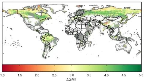
The spatial distribution of sensitivity of the biosphere to global warming is investigated in figure 4 using the median 1GMT at which 0 first exceeds the severe change threshold (0.3) across all GVMs for RCP 8.5. Together with the far northern boreal forests of Canada and Russia, some regions of the tundra and shrublands of the Tibetan Plateau, where warmer winters result in longer growing seasons, are projected to be at risk of severe change as early as 1GMT ≈ 1.5◦_{C. By1GMT ≈ 3}◦_{C, the savannah regions}

in the Horn of Africa, along with large boreal forest regions across northern Canada and northern Russia, the Amazon forest and the grasslands of south-eastern India are projected to be at risk of severe change.

However, individual maps of 0 for each GCM–GVM combination reveal large differences in the spatial distribution and intensity of ecosystem shifts (see figure S9–S12 for a full set of world maps, available at stacks.iop.org/ERL/8/ 044018/mmedia). In general, the uncertainty in the spatial distribution of risk of severe change coming from the GVMs is greater than from the GCMs (see section2.4). For example, the projections of changes in the savannah region in the Horn of Africa range from little to small change for JeDi with the HadGEM2-ES RCP 8.5, to values above 0.3 for LPJmL for the same climate forcing. Projections of the spatial extent and magnitude of 0 in the Tibetan Plateau also vary significantly across the GVMs, despite a similar projection of global land fraction at risk, ranging from widespread, severe change for SGVM for IPSL-CM5A-LR RCP 8.5, through to only small risk of ecosystem change according to ORCHIDEE for the same forcing. These regional differences highlight the importance of such analysis to identify where

Environ. Res. Lett. 8 (2013) 044018 L Warszawski et al

Figure 4. Median1GMT (averaged over a 30-year window), across all ecosystem models and RCP 8.5 climate runs (ensuring that all runs reach1GMT = 4◦_{C), at which the ecosystem is projected to first be at risk of severe change (0 > 0.3, during the period 1994–2084). Each}

pixel is coloured according to the median temperature across all RCP 8.5 GCM runs above which severe ecosystem change is projected. In the case that a severe change is not experienced, pixels are coloured grey. Where fractional vegetation cover is less than 2.5%, pixels remain white. Where more than half the models do not cross the0 = 0.3 threshold, pixels are coloured grey. White cells have either <50% naturally vegetated land surface according to [28] or<2.5% vegetation cover. The spread in the value of 0 arising from GCMs and ecosystem models is shown in figure5.

the differences in process implementation across the GVMs lead to the greatest discrepancy in projections of ecosystem change. Global aggregations such as reported in figure 3

should therefore be treated cautiously, as they can obscure the fact that these global values arise from significantly different spatial distributions of change.

2.4. Model agreement and uncertainty

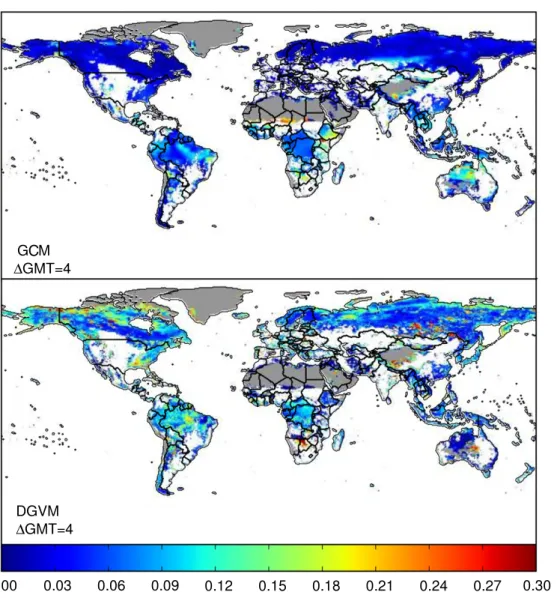
At1GMT = 4◦C (reached only using RCP 8.5; see table S3), the uncertainty in 0 arising from the GVMs is on average approximately twice as large as the uncertainty arising from the GCMs (shown as the standard deviation in 0 across GCMs and GVMs in the top and bottom panels of figure 5 respectively). The standard deviation across the ecosystem models is particular high in south-eastern North America, Turkey, south-east Australia, the Tibetan Plateau, south-east India, Canada and southern South America. In many of these regions, LPJmL and Hybrid project relatively large changes in vegetation composition, which cannot be mimicked in those models without dynamic vegetation composition. Additionally, differences across impact models are considerably more pronounced at 1GMT = 4◦C compared to 2◦C (see figure S16, available atstacks.iop.org/ ERL/8/044018/mmedia), in line with the conclusions drawn from figure2. Major differences in the behaviour of stomatal conductance in response to vapour pressure deficit may contribute to spread in the ecosystem models, in particular in tropical forests. Mortality is also handled differently across the models, which contributes to the factor of two difference in carbon residence times across the models [46], and contributes particularly strongly to the uncertainty in 0 projections in the northern latitude boreal forests. In addition, the shifts in this region are driven strongly by the response, among

other processes, of water-use efficiency to atmospheric CO2

concentration, which is shown in figure S3 (available at

stacks.iop.org/ERL/8/044018/mmedia) to vary greatly across the ecosystem models. Despite these differences in the magnitude of 0, at 1GMT = 4◦C approximately 60% of all combinations of ecosystem model and GCM project0 > 0.3 across the northern Amazon forest, southern India and the Tibetan Plateau (see figure S17 for the percentage of model runs agreeing on0 > 0.3 at different levels of global warming, available atstacks.iop.org/ERL/8/044018/mmedia). Uncertainty in the projections of risk of ecosystem change arising from the GCMs dominates the Sahel region, where the median temperature at which the median 0 first exceeds 0.3 is 2.5◦C< 1GMT < 3.5◦C and water fluxes dominate0 (see figure1).0 in the monsoon region of India is also dominated by uncertainty arising from the GCMs, where the relative change in discharge compared to present day is also projected to increase by over 30% based on multi-model projections conducted as part of ISI-MIP [49]. It is interesting to note that very few of the regions of projected risk of severe ecosystem change correspond to regions projected to get drier under climate change. This most likely arises from the increased water-use efficiency of plants under elevated atmospheric CO2, which help to counter this effect.

2.5. Biodiversity hotspots

In many cases, the regions projected to be threatened by severe ecosystem change at 1GMT > 2◦C coincide with regions that harbour exceptional biodiversity according to ‘The Global 200’ (compiled by [42] and comprising 142 terrestrial regions, see figure S18, available atstacks.iop.org/ ERL/8/044018/mmedia). This set of regions was selected by analysing patterns of biodiversity to identify distinctive and

Figure 5. Spread in0 across GCMs (top) and ecosystem models (EM, bottom) at 1GMT = 4◦C for the RCP 8.5 runs. The EM (GCM) values are calculated by averaging the standard deviation over all GVM (GCM) runs around the mean for each GCM (GVM) at each pixel. Figure S16 (available atstacks.iop.org/ERL/8/044018/mmedia) shows the spread for1GMT = 2◦C. White cells have<50% naturally vegetated land surface according to [28] and grey cells have<2.5% vegetation cover.

irreplaceable biomes and biogeographic realms, whilst relying on the discretion of the authors to make a final selection. The assessment accounts for species richness and endemic species, as well as unusual ecological or evolutionary phenomena and rarity of global habitats. Regions of overlap between projected risk of severe ecosystem changes and regions of exceptional biodiversity are myriad, including the montane grass and shrublands of the Tibetan Plateau Steppe and the Kamchatka Taiga and Grasslands in north-eastern Russia. Several moist forest regions also overlap with regions of projected severe change, including the Guayanan Highland Moist forests and Amazon forests, and the moist and dry forests of north-eastern India. The Cerrado woodlands south-east of the Amazon basin, constituting one of the largest savanna forest complexes in the world, coincide with an area where the median projects risk of severe ecosystem changes at 3◦C< 1GMT < 4◦C. In a similar temperature range, the Acacia Savannas in the Horn of Africa and the Northern Australian and Trans-Fly Savannas also overlap with model predictions of risk of severe ecosystem shifts.

2.6. Response to regional temperature and precipitation changes

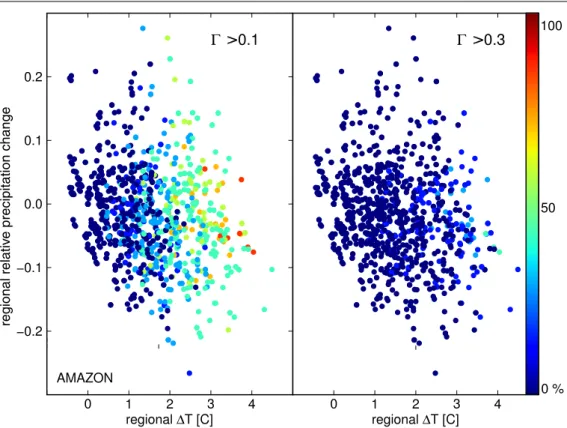
On the regional scale, we can relate 0 to local changes in precipitation and temperature patterns. Taking the much-studied moist Amazon forest as an example [43, 44], in figure 6 we plot the percentage of ecosystem models that agree on a risk of moderate (left) and severe (right) ecosystem change in the Amazon region for each year of each combination of RCP and GCM. Unlike in [45], where a strong trend in the plant functional type composition change with both regional precipitation and temperature change was projected, no trend is visible here. Note that relative precipitation changes here are limited to ≤20%. The strong trend in agreement with increasing regional absolute temperature change is most likely driven by increased vegetation carbon stocks due to CO2 fertilization effects

(see figure1and [46]). It is also important to note that0 is not only a measure of dieback or greening (although both Hybrid and LPJmL project a decline in Amazon rainforest trees [46]),

Environ. Res. Lett. 8 (2013) 044018 L Warszawski et al

Figure 6. Percentage of models that project a risk of small (left) and severe (right) ecosystem change as a function of relative regional precipitation change and absolute regional temperature change in the Amazon forest.0 is averaged over the same region as the temperature and precipitation changes. Each point gives the percentage of models that project a small or severe risk of change in a given year. The individual plots for each ecosystem model are shown in figure S15 (available atstacks.iop.org/ERL/8/044018/mmedia).

but rather of the aggregated biogeochemical biomes changes. A similar approach to regional analysis of ecosystem shifts could be extended to develop regional ecosystem impact functions, facilitating inclusion of risk of ecosystem change in globally aggregated and sectorally integrated models.

3. Conclusions

The balance of carbon and water fluxes and stores, together with vegetation composition, help to define the unique biogeochemical conditions of an ecosystem. In this study we have presented a summary of a multi-model, global investigation of the risk of climate change driven changes in these properties, which we have interpreted as risks of ecosystem shifts at different levels of global warming. The seven participating ecosystems models report a broad range of projections under future climate change scenarios, both in terms of the spatial distribution of changes, as well as their magnitude. Large discrepancies in both the globally aggregated level of risk of ecosystem change, and its geographical distribution arise from the diversity of processes implemented and their sensitivities to climate changes and increasing atmospheric CO2 concentrations, where the

uncertainty is dominated in most regions by the uncertainty arising from the GVMs rather than the climate input. Despite the large uncertainty in results, the model ensemble agrees on an increasing risk of severe change globally under all warming scenarios considered, with a doubling in the median

naturally vegetated land surface area at risk of severe change between 1GMT = 2 and 3◦C (compared to 1980–2010). Therefore, this study represents an important first step towards multi-model, multi-scenario assessments of the risks of ecosystem shifts under climate change. However, further investigation is required to understand the full extent of impact of biogeochemical shifts on highly networked ecosystems.

A more concrete projection of the regions at greatest risk of ecosystem change and the inherent uncertainties requires greater consistency across the models in the biogeochemical processes represented, and in particular a careful treatment of the response of these processes to elevated atmospheric CO2

concentrations. Studies such as presented in [46] where it is shown that discrepancies in residence times across the models is the major contributor to differences in vegetation carbon across the model ensemble, are essential contributions to our understanding of the risks posed to ecosystems by climate change. Representation of dynamic vegetation composition changes in all models, and expansion of the study to include other models that already include these changes, would also provide for a more consistent informative multi-model approach. Identification and reduction of individual sources of uncertainty are thus necessary steps towards a better understanding of ecosystem changes due to climate change, and towards addressing urgent questions about the impact of climate change of Earth’s ecosystems and the human societies that depend on them.

Acknowledgments

This work has been conducted under the framework of ISI-MIP. The ISI-MIP Fast Track project underlying this paper was funded by the German Federal Ministry of Education and Research (BMBF) with project funding reference number 01LS1201A. Responsibility for the content of this publication lies with the author. KF was supported by the Federal Ministry for the Environment, Nature Conservation and Nuclear Safety (11 II 093 Global A SIDS and LDCs). RK was supported by the Joint DECC/Defra Met Office Hadley Centre Climate Programme (GA01101). AI and KN were supported by the Environment Research and Technology Development Fund (S-10) of the Ministry of the Environment, Japan. Ron Kahana was supported by the Joint DECC/Defra Met Office Hadley Centre Climate Programme (GA01101). FP received funding from the European Union’s Seventh Framework Programme [FP7/2007–2013] under grant agreement no. 266992. The authors acknowledge the World Climate Research Programme’s Working Group on Coupled Modelling, which is responsible for CMIP, and thank the climate modeling groups (HadGEM2-ES, IPSL-CM5A-LR, MIROC-ESM-CHEM, GFDL-ESM-2M, and NorESM1-M) for producing and making available their model output.

References

[1] Burrows M T et al 2011 Science334 652–5

[2] Jones C, Lowe J, Liddicoat S and Betts R 2009 Nature Geosci.

2 484–7

[3] Mooney H, Larigauderie A, Cesario M, Elmquist T, Hoegh-Guldberg O, Lavorel S, Mace G M, Palmer M, Scholes R and Yahara T 2009 Curr. Opin. Environ. Sustain.

1 46–54

[4] Jentsch A and Beierkuhnlein C 2008 External Geophys. Clim. Environ.340 621–8

[5] Finzi A C, Austin A T, Cleland E E, Frey S D, Houlton B Z and Wallenstein M D 2011 Front. Ecol. Environ.9 61–7

[6] Hooper D U, Adair E C, Cardinale B J, Byrnes J E K, Hungate B A, Matulich K L, Gonzalez A, Duffy J E, Gamfeldt L and O’Connor M I 2012 Nature486 105–8

[7] Warren R, Price J, Fischlin A, Nava Santos S and Midgley G 2010 Clim. Change106 141–77

[8] Montoya J M and Raffaelli D 2010 Phil. Trans. R. Soc. B

365 2013–8

[9] Friedlingstein P et al 2006 J. Clim.19 3337–53

[10] Cramer W et al 2001 Glob. Change Biol.7 357–73

[11] Randerson J T et al 2009 Glob. Change Biol.15 2462–84

[12] Sitch S et al 2008 Glob. Change Biol.14 2015–39

[13] Scholze M, Knorr W, Arnell N W and Prentice I C 2006 Proc. Natl Acad. Sci. USA103 13116–20

[14] Ostberg S, Lucht W, Schaphoff S and Gerten D 2013 Earth Syst. Dyn.4 347–57

[15] Heyder U, Schaphoff S, Gerten D and Lucht W 2011 Environ. Res. Lett.6 034036

[16] Bradshaw W E and Holzapfel C M 2006 Science312 1477–8

[17] Harmon J P, Moran N A and Ives A R 2009 Science

323 1347–50

[18] Nemani R R, Keeling C D, Hashimoto H, Jolly W M, Piper S C, Tucker C J, Myneni R B and Running S W 2003 Science300 1560–3

[19] Myneni R B, Keeling C D, Tucker C J, Asrar G and Nemani R R 1997 Nature386 698–702

[20] Buitenwerf R, Bond W J, Stevens N and Trollope W S W 2012 Glob. Change Biol.18 675–84

[21] Elmendorf S C et al 2012 Nature Clim. Change2 453–7

[22] Moss R H et al 2010 Nature463 747–56

[23] Warszawski L, Frieler K, Huber V, Piontek F, Schewe J and Serdeczny O 2013 Proc. Natl Acad. Sci. at press (doi:10.1073/pnas.1312330110)

[24] Falloon P and Betts R 2010 Sci. Tot. Environ.408 5667–87

[25] Blois J L, Williams J W, Fitzpatrick M C, Jackson S T and Ferrier S 2013 Proc. Natl Acad. Sci. USA (doi:10.1073/ pnas.1220228110)

[26] Hempel S, Frieler K, Warszawski L, Schewe J and Piontek F 2013 Earth Syst. Dyn.4 219–36

[27] Meinshausen M et al 2011 Clim. Change109 213–41

[28] Portmann F T, Siebert S and D¨oll P 2010 Glob. Biogeochem. Cycles24 GB1011

[29] Pavlick R, Drewry D T, Bohn K, Reu B and Kleidon A 2012 Biogeosci.10 4137–77

[30] Woodward F I and Lomas M R 2004 Biol. Rev.79 643–70

[31] Beerling D J, Fox A, Stevenson D S and Valdes P J 2011 Proc. Natl Acad. Sci. USA108 9770–5

[32] Inatomi M, Ito A, Ishijima K and Murayama S 2010 Ecosystems13 472–83

[33] Best M J et al 2011 Geosci. Model Dev.4 677–99

[34] Clark D B et al 2011 Geosci. Model Dev.4 701–22

[35] Friend A D and White A 2000 Glob. Biogeochem. Cycles

14 1173

[36] Sitch S et al 2003 Glob. Change Biol.9 161–85

[37] Gerten D, Schaphoff S, Haberlandt U, Lucht W and Sitch S 2004 J. Hydrol.286 249–70

[38] Krinner G 2005 Glob. Biogeochem. Cycles19 GB1015

[39] Piao S, Friedlingstein P, Ciais P, de Noblet-Ducoudr´e N, Labat D and Zaehle S 2007 Proc. Natl Acad. Sci. USA

104 15242–7

[40] Davie J C S et al 2013 Earth Syst. Dyn. Discuss.4 279–315

[41] Cao L and Caldeira K 2010 Environ. Res. Lett.5 024011

[42] Olson D and Dinerstein E 2002 Ann. Mo. Bot. Gard.

89 199–224

[43] Rammig A, Jupp T, Thonicke K, Tietjen B, Heinke J, Ostberg S, Lucht W, Cramer W and Cox P 2010 New Phytol.187 694–706

[44] Malhi Y, Arag˜ao L E O C, Galbraith D, Huntingford C, Fisher R, Zelazowski P, Sitch S, McSweeney C and Meir P 2009 Proc. Natl Acad. Sci. USA106 20610–5

[45] Cowling S A and Shin Y 2006 Glob. Ecol. Biogeogr.553–66

[46] Friend A et al 2013 Proc. Natl Acad. Sci. at press (doi:10.1073/pnas.12222477110)

[47] Piontek F et al 2013 Proc. Natl Acad. Sci. USA at press (doi:10.1073/pnas.1222471110)

[48] Frieler K et al 2013 in preparation

[49] Schewe J et al 2013 Proc. Natl Acad. Sci. at press (doi:10.1073/pnas.1222460110)