HAL Id: hal-01190133
https://hal.archives-ouvertes.fr/hal-01190133
Submitted on 28 May 2020
HAL is a multi-disciplinary open access
archive for the deposit and dissemination of
sci-entific research documents, whether they are
pub-lished or not. The documents may come from
teaching and research institutions in France or
abroad, or from public or private research centers.
L’archive ouverte pluridisciplinaire HAL, est
destinée au dépôt et à la diffusion de documents
scientifiques de niveau recherche, publiés ou non,
émanant des établissements d’enseignement et de
recherche français ou étrangers, des laboratoires
publics ou privés.
stand-replacing fire disturbance: insights from a global
process-based vegetation model
C. Yue, P. Ciais, S. Luyssaert, P. Cadule, J. Harden, J. Randerson, Valentin
Bellassen, T. Wang, S. L. Piao, B. Poulter, et al.
To cite this version:
C. Yue, P. Ciais, S. Luyssaert, P. Cadule, J. Harden, et al.. Simulating boreal forest carbon dynamics
after stand-replacing fire disturbance: insights from a global process-based vegetation model:
Simu-lating boreal forest carbon dynamics after stand-replacing fire disturbance. Biogeosciences, European
Geosciences Union, 2013, 10 (12), pp.8233. �10.5194/bg-10-8233-2013�. �hal-01190133�
www.biogeosciences.net/10/8233/2013/ doi:10.5194/bg-10-8233-2013
© Author(s) 2013. CC Attribution 3.0 License.
Biogeosciences
Simulating boreal forest carbon dynamics after stand-replacing fire
disturbance: insights from a global process-based vegetation model
C. Yue1, P. Ciais1, S. Luyssaert1, P. Cadule1, J. Harden2, J. Randerson3, V. Bellassen4, T. Wang1, S. L. Piao5, B. Poulter1, and N. Viovy1
1Laboratoire des Sciences du Climat et de l’Environnement, UMR8212, LSCE CEA CNRS UVSQ, 91191 Gif-sur-Yvette,
France
2US Geological Survey, Menlo Park, CA, USA
3Department of Earth System Science, University of California, Irvine, California, USA
4CDC Climat, 47 rue de la Victoire, 75009 Paris, France
5Department of Ecology, College of Urban and Environmental Science, Peking University, Beijing 100871, China
Correspondence to: C. Yue ([email protected])
Received: 12 March 2013 – Published in Biogeosciences Discuss.: 24 April 2013 Revised: 30 October 2013 – Accepted: 9 November 2013 – Published: 13 December 2013
Abstract. Stand-replacing fires are the dominant fire type in North American boreal forests. They leave a historical legacy of a mosaic landscape of different aged forest cohorts. This forest age dynamics must be included in vegetation models to accurately quantify the role of fire in the histori-cal and current regional forest carbon balance. The present study adapted the global process-based vegetation model
ORCHIDEE to simulate the CO2emissions from boreal
for-est fire and the subsequent recovery after a stand-replacing fire; the model represents postfire new cohort establishment, forest stand structure and the self-thinning process. Simula-tion results are evaluated against observaSimula-tions of three clus-ters of postfire forest chronosequences in Canada and Alaska.
The variables evaluated include: fire carbon emissions, CO2
fluxes (gross primary production, total ecosystem respira-tion and net ecosystem exchange), leaf area index, and bio-metric measurements (aboveground biomass carbon, forest floor carbon, woody debris carbon, stand individual density, stand basal area, and mean diameter at breast height). When
forced by local climate and the atmospheric CO2 history
at each chronosequence site, the model simulations
gener-ally match the observed CO2 fluxes and carbon stock data
well, with model-measurement mean square root of deviation
comparable with the measurement accuracy (for CO2 flux
∼100 g C m−2yr−1, for biomass carbon ∼ 1000 g C m−2and for soil carbon ∼ 2000 g C m−2). We find that the current postfire forest carbon sink at the evaluation sites, as observed
by chronosequence methods, is mainly due to a combina-tion of historical CO2increase and forest succession. Climate change and variability during this period offsets some of these expected carbon gains. The negative impacts of climate were a likely consequence of increasing water stress caused by significant temperature increases that were not matched by concurrent increases in precipitation. Our simulation re-sults demonstrate that a global vegetation model such as OR-CHIDEE is able to capture the essential ecosystem processes in fidisturbed boreal forests and produces satisfactory re-sults in terms of both carbon fluxes and carbon-stock evo-lution after fire. This makes the model suitable for regional simulations in boreal regions where fire regimes play a key role in the ecosystem carbon balance.
1 Introduction
Boreal forests store a large amount of the global terrestrial-ecosystem carbon, with 78 Pg C in biomass and ∼ 230 Pg C in soil (Kasischke, 2000). This forest biome has been esti-mated to be a carbon sink over the late 20th century (Kurz and Apps, 1999; McGuire et al., 2009; Pan et al., 2011), but the carbon stock and carbon sink are highly sensitive to fire disturbance (Balshi et al., 2009; Bond-Lamberty et al., 2007b). Particularly, forests in boreal North America ap-peared likely to become a carbon source in the past decade
due to increased fire and insect disturbances (Hayes et al., 2011; Stinson et al., 2011). Stand-replacing fires are the ma-jor natural disturbance in the North American boreal forest and thus fire frequency and severity, and their changes, play a key role in controlling large-scale boreal forest carbon dy-namics (Balshi et al., 2007; Bond-Lamberty et al., 2007b; Harden et al., 2000; Hayes et al., 2011).
A long-term ecological consequence of stand-replacing fire is that trees are generally completely killed (although with a possible delay in time) and a large amount of snags are left to decompose (Amiro et al., 2006; Liu et al., 2005; Manies et al., 2005), while a secondary ecosystem succession is initiated, with a new forest cohort being established (Ka-sischke et al., 1995). Time-since-disturbance is an ecosys-tem state variable which is often important in determining the carbon flux and carbon stock (Litvak et al., 2003; Pregit-zer and Euskirchen, 2004; Amiro et al., 2006, 2010). Forest age is recognized as a key factor in explaining the sign and magnitude of the carbon balance of North American boreal forests (Kurz and Apps, 1999; Kurz et al., 2009; Stinson et al., 2011). Besides fluxes, fire and forest age may also im-pact the pattern of land–atmosphere water and energy ex-change (Liu and Randerson, 2008; Liu et al., 2005). Thus, to simulate the effects of fire disturbance on the regional car-bon balance and biophysical changes, these stand-age effects must be included in general purpose, large-scale vegetation models.
Since the 1970s, boreal forests have experienced a sig-nificant temperature rise and probably an intensifying fire regime (Euskirchen et al., 2007; Kasischke and Turetsky, 2006). A plethora of modeling studies have investigated how the historical carbon stock of boreal forest has changed in
re-sponse to changes in climate, atmospheric CO2and the fire
regime (Balshi et al., 2007; Bond-Lamberty et al., 2007b; Hayes et al., 2011; Yuan et al., 2012). There is general
agree-ment that increasing atmospheric CO2tends to favor carbon
accumulation in the system, while fires exert a negative ef-fect on the net terrestrial carbon sink, but the role of tem-perature rise is uncertain. Satellite-derived evidence indicates that rising temperature generally increases the length of the thermal growing season; however, the carbon uptake result-ing from the earlier growresult-ing season onset is partly offset by warming in the fall due to enhanced respiration (Barichivich et al., 2012; Piao et al., 2008). Despite all these efforts, the effects of climate variability and increased atmospheric CO2 on postfire forest carbon flux trajectories have not been ex-amined at the site level, using a model-observation combined approach within the context of postfire forest succession.
Here, we use a general process-based global vegetation model to simulate postfire forest carbon dynamics. After fire, the model establishes a new forest cohort with explicit stand structure, and simulates forest dynamics such as self-thinning and snag decomposition. Carbon flux and carbon stock data from 13 flux sites across North American boreal forests are used for comprehensive model calibration and
er-ror characterization. The role of historical climate and at-mospheric CO2trend in driving the postfire carbon flux tra-jectory is explored by model manipulation in combination with in situ measurements. Specifically, the objectives of this study are:
– to perform a calibration of the model by adjusting its
parameters simultaneously against CO2 fluxes (gross
primary production or GPP, net ecosystem production or NEP, total ecosystem respiration or TER), and on carbon stocks (total and aboveground biomass carbon stock, forest floor carbon stock, woody debris carbon, mineral soil carbon), and forest stand structure (basal area, stand density, mean diameter at breast height, or DBH);
– to evaluate the model performance at different sites across different soil drainage conditions;
– to attribute the effects of climate and atmospheric CO2 trends in driving the postfire trajectory carbon fluxes at the sites examined;
– to quantify the uncertainty in CO2fluxes and the resid-ual model biases which cannot be reduced by calibra-tion, in order to assess the modeled carbon balance un-certainty for regional-scale applications.
2 Materials and methods
2.1 Site descriptions
Details of the three clusters of chronosequence sites dis-tributed across the boreal forest biome in North America are given in Table 1. The sites include three flux towers (US-Bn1 to US-Bn3) in Alaska, USA, seven flux towers (CA-NS1 to CA-NS7) in western Manitoba, Canada, and another three flux towers (CA-SF1 to CA-SF3) in Saskatchewan, Canada. The climate conditions differ among the three
clus-ters, with mean annual temperatures (MAT) of −2.1◦C for
Alaska,−3.2◦C for Manitoba and 0.4◦C for Saskatchewan.
Mean annual precipitation (MAP) is 290 mm for Alaska, 536 mm for Manitoba and 470 mm for Saskatchewan.
The year of the most recent fire event is available for all these sites. The eddy-covariance (EC) method was used to measure CO2fluxes for different times after fire disturbance (Table 1). For clarity, the fire events listed in Table 1 are here-inafter referred to as “the most recent fire event”, and the pe-riods during which EC observations have been made are re-ferred to as “the EC observation period”. The individual EC measurement locations with multiple towers (US-Bn1-3/CA-NS1-7/CA-SF1-3) will be referred to as “evaluation site(s)”. All the study sites are documented to have experienced stand-replacing fires, with all aboveground biomass being killed in the fire, resulting in complete forest regeneration
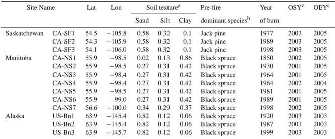
Table 1. Measurement sites used in this study for model evaluation, their geographical coordinates, soil texture, pre-fire dominant vegetation
species, year of the most recent fire event, and the period of eddy-covariance observation.
Site Name Lat Lon Soil texturea Pre-fire Year OSYc OEYc Sand Silt Clay dominant speciesb of burn
Saskatchewan CA-SF1 54.5 −105.8 0.58 0.32 0.1 Jack pine 1977 2003 2005 CA-SF2 54.3 −105.9 0.58 0.32 0.1 Jack pine 1989 2003 2005 CA-SF3 54.1 −106.0 0.58 0.32 0.1 Jack pine 1998 2003 2005 Manitoba CA-NS1 55.9 −98.5 0.02 0.13 0.86 Black spruce 1850 2002 2005 CA-NS2 55.9 −98.5 0.27 0.31 0.42 Black spruce 1930 2001 2005 CA-NS3 55.9 −98.4 0.27 0.31 0.42 Black spruce 1964 2001 2005 CA-NS4 55.9 −98.4 0.27 0.31 0.42 Black spruce 1964 2002 2004 CA-NS5 55.9 −98.5 0.27 0.31 0.42 Black spruce 1981 2001 2005 CA-NS6 55.9 −99.0 0.27 0.31 0.42 Black spruce 1989 2001 2005 CA-NS7 56.6 −100.0 0.34 0.29 0.37 Black spruce 1998 2002 2005 Alaska US-Bn1 63.9 −145.4 0.82 0.12 0.06 Black spruce 1920 2003 2003 US-Bn2 63.9 −145.4 0.82 0.12 0.06 Black spruce 1987 2003 2003 US-Bn3 63.9 −145.7 0.82 0.12 0.06 Black spruce 1999 2003 2003 aSoil texture information, where available, is provided by site PIs, otherwise it is completed from the soil map of Zobler (1986) and translated into sand/silt/clay fractions by the model default values that correspond to soil types in the Zobler map.bBlack spruce: Picea mariana (Mill.) BSP; Jack pine: Pinus banksiana Lamb.cOSY, Eddy covariance observation period start year; OEY, Eddy covariance observation period end year.
(Amiro et al., 2006; Goulden et al., 2006; Liu and Ran-derson, 2008). Vegetation before burning was dominated by black spruce (Picea mariana (Mill.) BSP) or jack pine
(Pi-nus banksiana Lamb.), and was in various stages of forest
re-covery when measurements were collected. Dead tree boles were found to remain intact and upright until approximately 5 yr after fire, and most of these snags then fell within 10– 15 yr after burning (Goulden et al., 2006; Liu and Randerson, 2008). Soils at the three evaluation site clusters are moder-ately well-drained to well-drained (Gower et al., 1997; Liu et al., 2005; Goulden et al., 2006). Permafrost occurs at the Alaska and Manitoba sites but is absent for the top 2 m of soil for all the Saskatchewan sites (Gower et al., 1997).
The model was evaluated against various measurements collected from a range of published studies, or retrieved by the authors. Variables evaluated comprise GPP, NEP, TER, leaf area index (LAI), total (aboveground) biomass carbon, woody debris carbon, forest floor carbon, mineral soil car-bon, forest DBH, individual density, and basal area. The de-tailed data source information is provided in Table S1. 2.2 Model description of ORCHIDEE-FM
For our research objectives, the global general purpose, process-based vegetation model ORCHIDEE (Krinner et al., 2005) is used. Brought to steady equilibrium state for vege-tation and soil carbon pools after a long spinup, ORCHIDEE originally represents an “average” mature forest in a big-leaf approximation. To explicitly account for forest stand structure and processes related with forest age, a forest management module (FM) was developed (Bellassen et al., 2010). The version of ORCHDEE with FM module is here-inafter referred to as “ORCHIDEE-FM”, and the original
ORCHDEE (without FM) will be referred to as “the standard ORCHIDEE”.
ORCHIDEE-FM includes several processes that are im-portant in simulating forest stand development: (1) age-related stand dynamics, including the decline in NPP in old forests, age limitation of LAI growth in young stands, and age-dependent allocation of woody NPP among stems and coarse roots; (2) a woody litter pool to account for the slow decomposition of that material; and (3) an explicit descrip-tion of forest stand structure (stand density, tree diameter distribution, etc.) with the model able to simulate the self-thinning process, given a maximum density–biomass rela-tionship for different types of forests.
The decomposition for above- and belowground litter and mineral soil organic carbon is modeled to follow a first-order kinetic equation in ORCHIDEE-FM (Parton et al., 1988). Acknowledging the different turnover rates of its compo-nents, the litter pool is sub-divided into metabolic, struc-tural and woody litter. Plant live biomass is divided into eight compartments: leaf, above- and belowground sapwood, above- and belowground heartwood, root, fruit, and carbon reserve pool. In ORCHIDEE-FM, when carbon is transferred from the live biomass to the litter pools, the carbon from live biomass does not go directly to the three litter pools, it goes first to a temporary litter buffer, and is then allocated to the three litter pools according to prescribed ratios (Krinner et al., 2005).
2.3 Modifications of ORCHIDEE-FM into ORCHIDEE-FM-BF for boreal fires
ORCHIDEE-FM was adapted into ORCHIDEE-FM-BF (ORCHIDEE-FM for Boreal Fires) to make it able to
simulate boreal crown fire processes. A crown fire kills all the aboveground biomass and initiates a new forest cohort, and is similar to a clear-cut event from a successional modeling per-spective, although the aboveground carbon is exported in the case of clear-cut. The “clear-cut” routine of the FM module was thus adapted to mimic fire burning effects and the es-tablishment of new forest after fire. When crown fire occurs, part of the ground litter and tree biomass are removed from existing pools as carbon emissions into the atmosphere, and the unburned biomass is simulated as standing dead wood (snags), which gradually moves into the litter pool over time. 2.3.1 Age-related changes of LAI and productivity
Previous studies have reported that LAI increases with stand age in young boreal forests until ∼ 25 yr; after that LAI tends to saturate (Wang et al., 2003; Goulden et al., 2011). This age dependence of LAI is empirically modeled by scaling the maximum LAI (a parameter specified for each biome in ORCHIDEE which sets an achievable climax LAI, not nec-essarily reached at a given site) to increase with the square root of stand age until 25 yr. The model’s default maximum LAI of 4.5 m2m−2for the boreal forest biome was used.
To account for the productivity decrease in aging bo-real forests (Bond-Lamberty et al., 2004; Mack et al., 2008; Goulden et al., 2011), a decrease in the optimal carboxyla-tion rate in old-growth forest was added to the model. For stands aged between 100 and 200 years old, the optimal car-boxylation rate is modeled to decrease by up to 10 % over the 100 yr in a linear way, to mimic the NPP reduction between the 74 and 154 year old forests in central Canada observed by Goulden et al. (2011). To promote agreement between the simulated and field-based estimates of productivity, the op-timal carboxylation rate was adjusted from the default value of 35 µmol m−2s−1to 24 µmol m−2s−1.
2.3.2 Fire combustion fraction for different carbon pools
In fires of boreal North America, carbon emissions come mainly from ground fuel (or organic soil horizons) and live biomass combustion is limited to tree leaves and small branches. The combustion fraction depends on a range of factors and is not necessarily constant; however, the present study was not seeking an accurate simulation of the combus-tion process and thus simple fixed combuscombus-tion fraccombus-tions were adopted for different types of fuel. Considering the data in available field reports (Stocks, 1987, 1989; Kasischke and Stocks, 2000; Kasischke and Hoy, 2012), the combustion fraction was set to 7 % for aboveground live biomass and 30 % for ground litter. The unburned biomass was transferred to the snag pool (see Supplement Sect. 1 for more detailed description).
2.3.3 Snag decay after a fire event
At the three study sites, fire-formed snags and downed dead-wood represent a significant component of the forest carbon stocks. In reality, the decrease of snags (either standing or downed) occurs through three processes: decomposition by microbes, fragmentation and leaching. Field measurements show that the change of snag and woody debris as a func-tion of time after fire follows a first-order kinetic equafunc-tion (Bond-Lamberty and Gower, 2008):
dD
dt = −kD, (1)
where dDdt is the change of woody debris, D is the
exist-ing woody debris and k is the annual decomposition con-stant. Bond-Lamberty and Gower (2008) reported a k value
of 0.05–0.07 yr−1for standing snag and downed woody
de-bris using three independent methods: direct respiration mea-surement, repeated field surveys and chronosequence obser-vation.
To represent this process, a snag pool was added in ORCHIDEE-FM-BF, which includes the aboveground un-burned heartwood biomass and belowground thick pivotal woody roots. To simplify the model, it was assumed that no respiration occurs for standing snags and that the reduced snag mass enters the litter pool completely. This is consistent with the results of Manies et al. (2005), who found standing snags (stems) respire very slowly until they fall and come into contact with moss and soil.
During the first 20 yr after fire, we assumed an annual de-cay rate of 8 % (k = 0.08 yr−1)of snag being transferred to the litter pool, and during the next 20–40 yr an annual rate of 5 % (k = 0.05 yr−1). Forty years after fire, all the remaining snag becomes litter. These parameters are derived from the field measurements by Bond-Lamberty and Gower (2008). 2.3.4 Modifying litter and soil carbon turnover time
The default values of litter and soil carbon turnover time in ORCHIDEE were originally defined from the CENTURY soil carbon decomposition model (Parton et al., 1988), which was based on grassland ecosystems. We modified the resi-dence time parameters in ORCHIDEE-FM-BF according to observations of radiocarbon content (Trumbore and Harden, 1997) and mass balance constraint studies (Harden et al., 2000; O’Donnell et al., 2011) for boreal soils. When driven by local climate, the modified mass weighted mean turnover time is ∼ 63 yr for aboveground litter (against 15.7 yr in the standard version of ORCHIDEE) and ∼ 2100 yr (against 1555 yr) for the mineral soil carbon pool.
2.4 Simulation set-up
2.4.1 Climate forcing data
Two sets of climate data are used for climate forcing. Composite Monthly Climate Data (hereafter referred to as CMCD) include monthly temperature and precipitation from meteorological stations close to the evaluation sites with the missing fields being filled by CRU3.1 data. Half-hourly climate data (hereafter referred to as HHCD) include gap-filled in situ meteorological measurements from the eddy-covariance sites (see Supplement Sect. 2 for more detailed description).
2.4.2 Vegetation, soil and other input data
ORCHIDEE-FM-BF is built on the concept of plant func-tional types (PFTs), with each PFT being associated with a specific vector of model parameters. Boreal evergreen needleleaf forests (black spruce or jack pine) are the climax vegetation type on the evaluation sites, although broadleaf trees such as trembling aspen often dominate at the early succession stage. The dynamic vegetation mechanisms in ORCHIDEE-FM-BF do not allow the realistic representa-tion of this species shift at the intermediate forest stage on a single simulation pixel, thus each site is prescribed to be fully covered by the boreal needleleaf evergreen forest PFT (see Krinner et al., 2005). The PFT-specific parameters in ORCHIDEE-FM-BF are set to the model default values given by Krinner et al. (2005) except the modifications de-scribed in Sect. 2.3. Soil texture is prede-scribed at each site as shown in Table 1.
2.4.3 Simulation protocol
Our simulations are conducted in a way that does not require specific biometric measurement inputs (such as LAI, initial biomass, mineral soil carbon etc.). Rather, these variables are determined from climate forcing data and the model equa-tions in a prognostic way, by starting with a spinup simula-tion followed with transient simulasimula-tions. Boreal forests are known to experience recurrent fire disturbances, and simi-larly, our simulation protocol is designed to allow a gradual ecosystem carbon pool accumulation under recurrent fires until equilibrium state, before the most recent fire event is simulated at each site (Fig. 1).
As we did not know the exact history of fire disturbance for each evaluation site, the fire return interval (FRI) for all the sites was set uniformly to be 160 yr. This value was cho-sen for three reasons. First, the oldest stand in the evalua-tion sites is 155 yr after fire (CA-NS1 in Manitoba). Second, the FRI for Canadian central boreal forest was reported to range between 66 and 200 yr by Stocks et al. (2002). Third, Anderson et al. (2006) reported that during the past 4600 yr, the FRI for a lowland boreal forest in south central Alaska was 142 ± 70 yr. We acknowledge that assuming a uniform
FRI of 160 yr is a simplification, as fire occurrence depends on several factors including climate (which varied during the Holocene) and the availability of fuel – thus not necessarily occurred at the equal intervals in the past.
According to the defined simulation protocol (Fig. 1), the model was initially run for a “first spinup” period starting from bare soil and without fires for 400 yr, followed by a “second spinup” of 3200 yr, i.e., 20 successive “fire rota-tions” with assumed stand-replacing fires occurring every 160 yr (each 160 yr period is called a “fire rotation”). This second spinup allows all forest ecosystem carbon pools (es-pecially the mineral soil carbon pool) to reach a long-term equilibrium state in the presence of recurrent fire disturbance. Finally, the most recent fire event is simulated for the year of burning. The model is then driven with actual climate forcing data during the postfire period of forest regrowth, so that the model output can be compared to and evaluated against field measurements.
We define a “climate forcing history” which was used by most of the simulations. The monthly CMCD climate data were used in this climate forcing history. The rationale of the climate forcing history was to ensure that, for the histor-ical spinup, the average state of historhistor-ical climate was used, and for the period before and after the most recent fire event, actual observed climate data were used. Specifically, the cli-mate forcing data used in different stages of the simulation protocol are as below (see also Table S2):
a. For the first spinup and the first 19 fire rotations of the second spinup, we use the multi-year mean CMCD climate data of each site from the first year of mete-orological station measurements until the year of the most recent fire (see Table S2 for details). This sta-ble climate forcing was used with the goal of driving the model into an equilibrium with the average state of historical climate conditions.
b. For the last (20th) fire rotation of the second spinup, at the beginning the average CMCD were used, but when entering the period of meteorological station measure-ment, the climate forcing shifted to actual year data. The time of shift depended on the year of the most recent fire and the duration of meteorological station observation at each site. By doing so, we made sure that before the most recent fire, actual monthly climate data were used to reflect the historical climate trends and variability that the ecosystem experienced at each site (see Table S2 for details).
c. For the postfire simulation after the most recent fire event, actual CMCD climate data continued to be used. But if the most recent fire occurred earlier than the start year of the meteorological station measurement, the average CMCD data were repeated until the year when meteorological station observations started and then real CMCD data began to be used.
Simulation Protocol
2 3
…
19 201
First spinup Secondspinup Postfiresimulation
Most recent fire EC observation
period
Average historical climate data Actual year climate data Constant 1850 CO2 Transient CO2 CNT-CMCD
ORC-STD FM-BF-NOSNAG
Average historical climate data Actual year climate data
GPPCAL-CMCD
Average historical climate data Actual year climate data Constant 1850 CO2
CO2FIX-CLIMVAR
160-year “fire rotation”
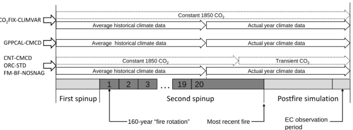
Fig. 1. Illustration of the simulation protocol, climate forcing and atmospheric CO2forcing data for various simulations. First spinup: the model is first run for 400 yr starting from bare soil without fire; second spinup: after first spinup, the model is run for 3200 yr, which consists of 20 successive “fire rotations” with assumed crown fires occurring every 160 yr (i.e., a FRI of 160 yr). Postfire simulation: the most recent fire event is simulated during the occurrence year, and the model is driven with actual observed climate forcing data for postfire regrowth. For clarity, CNT-HHCD, GPPCAL-HHCD and CO2FIX-CLIMFIX simulations were not shown. Refer to Sect. 2.4.4 and Table 2 for more detailed descriptions of different simulations.
Two scenarios of atmospheric CO2concentration were used
in the simulations, namely fixed CO2(CO2FIX) and variable
CO2(CO2VAR). For the CO2FIX scenario, the atmospheric
CO2 concentration was fixed at the 1850 level (285 ppm)
throughout the simulation. For the CO2VAR scenario, for the “first spinup” until the beginning of the 20th fire rotation of
the second spinup, CO2concentration was fixed at the 1850
level, then during the 20th fire rotation, beginning from some
point the atmospheric CO2was prescribed to increase
(tran-sient CO2concentration was used), and corresponded exactly
to the CO2concentration at the year of burning for the most recent fire at each site. This was done to reflect the atmo-spheric CO2history experienced at each individual site. The
difference between CO2VAR and CO2FIX allowed us to
sep-arate the effect of CO2fertilization on postfire CO2fluxes. 2.4.4 List of simulations in this study
Based on the defined simulation protocol, several simulations were performed; these are listed in Table 2 and described be-low:
CNT-CMCD: control simulation. The simulation was per-formed using ORCHIDEE-FM-BF with all the modified fea-tures, processes, and parameters described in Sect. 2.3. The
CO2VAR scenario was used.
GPPCAL-CMCD: GPP calibration simulation. This simu-lation used the same forcing as with the CNT-CMCD simula-tion, but the EC-observed multi-year mean GPP was assim-ilated (nudged) into the model. GPP assimilation was done by first calculating the ratio of average simulated to observed GPP at each study site for the EC observation period, and then applying this site-specific ratio throughout all the lation stages (first spinup, second spinup and postfire
simu-lation, see Fig. 1) to correct the simulated GPP for each run step. In this manner, the mean modeled GPP is tuned to be equal to the multi-year mean value observed by eddy covari-ance.
CNT-HHCD and GPPCAL-HHCD: these simulations are the same as CNT-CMCD and GPPCAL-CMCD, except that HHCD (half-hourly climate data) rather than CMCD were used during the EC observation period. Note that GPPCAL-CMCD and GPPCAL-HHCD simulations will have exactly the same GPP in every time step of the simulation (30 min) and the change from CMCD data to HHCD for the EC obser-vation period will only affect respiration, and thus net ecosys-tem production.
CO2FIX-CLIMVAR: no CO2fertilization simulation. The
CO2FIX scenario was used in the simulation, with varying
climate data.
CO2FIX-CLIMFIX: no CO2fertilization simulation. The
CO2FIX scenario was used in the simulation. But for the
postfire simulation after the most recent fire, input climate forcing was fixed as the average monthly climate data that was used in the spinup runs. This simulation, together with
CO2FIX-CLIMVAR simulation, was done only for sites
CA-NS1, CA-SF1 and US-Bn1, in order to be compared with the GPPCAL-CMCD simulation to separate the roles of
vary-ing climate and CO2 in the postfire carbon flux trajectory.
To make the results comparable with the GPPCAL-CMCD simulation, the same site-specific GPP correction ratio used in GPPCAL-CMCD simulation was applied to correct
mod-eled GPP in each step of the CO2FIX runs. This was done
for two reasons. First, this site-specific ratio is considered to reflect the model internal structural error that could not be resolved by parameterization and is therefore independent of
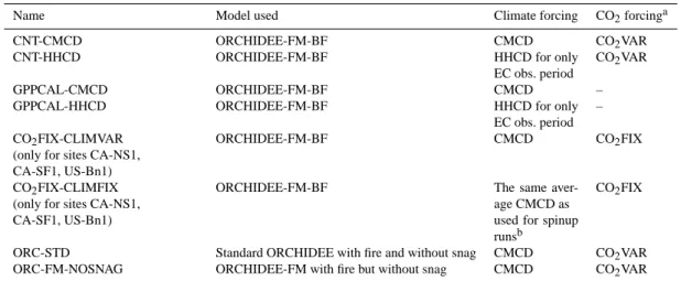
Table 2. List of simulations, and their climate and atmospheric CO2forcing.
Name Model used Climate forcing CO2forcinga
CNT-CMCD ORCHIDEE-FM-BF CMCD CO2VAR
CNT-HHCD ORCHIDEE-FM-BF HHCD for only
EC obs. period
CO2VAR
GPPCAL-CMCD ORCHIDEE-FM-BF CMCD –
GPPCAL-HHCD ORCHIDEE-FM-BF HHCD for only
EC obs. period –
CO2FIX-CLIMVAR
(only for sites CA-NS1, CA-SF1, US-Bn1)
ORCHIDEE-FM-BF CMCD CO2FIX
CO2FIX-CLIMFIX
(only for sites CA-NS1, CA-SF1, US-Bn1)
ORCHIDEE-FM-BF The same
aver-age CMCD as used for spinup
runsb
CO2FIX
ORC-STD Standard ORCHIDEE with fire and without snag CMCD CO2VAR
ORC-FM-NOSNAG ORCHIDEE-FM with fire but without snag CMCD CO2VAR
aAtmospheric CO
2forcing for GPPCAL-CMCD and GPPCAL-HHCD simulations is not applicable because GPP is externally forced to the model in the
simulation, by nudging mean multi-year observed annual GPP into the model.bFor the CO2FIX-CLIMFIX simulation, the average monthly climate data used are:
1968–1980(avg) for CA-NS1, 1943–1976(avg) for site CA-SF1, and 1930–1959(avg) for site US-Bn1 (see also Table S2).
scenario observation data available to derive the site-specific ratios.
ORC-STD: simulation with standard version of OR-CHIDEE. This simulation was done using the standard ver-sion of ORCHIDEE, with the same crown fire process as in Sect. 2.3 being implemented. No snag pool was represented and all unburned live biomass was sent to the litter pool (via the litter buffer) immediately after fire.
ORC-FM-NOSNAG: simulation with ORCHIDEE-FM with the same crown fire process implemented. Again, no fire caused snag process was represented in the model. This simulation and ORC-STD simulation were mainly for com-paring with the CNT-CMCD simulation to demonstrate the “improvement chain” in simulating postfire forest regrowth by moving from standard ORCHIDEE to ORCHIDEE-FM and further to ORCHIDEE-FM-BF.
2.5 Method for simulation-measurement comparison
Due to the differences in the scope of the forest floor, woody debris and mineral soil carbon as measured in the field and as modeled, a scheme was developed to match the model output with field measurements for these variables (refer to Supple-ment Sect. 3 for more details).
Three metrics were used to quantitatively evaluate the simulation-measurement agreement in a comprehensive way: 1. Metric 1. Linear regression was used to examine the overall model-measurement agreement. Simula-tion data were regressed against measurements with the regression line forced through the origin (regres-sion through origin; RTO) as it was assumed when the measurement value is zero, the simulation value should be zero as well. The RTO model used is
Yi =slope · Xi+εi, (2)
where Xi are measurement data, Yi are simulation
data, and εiis random error. If the regression slope was
not significantly different from unity, then we consid-ered it as fairly good agreement.
2. Metric 2. The root mean square deviation (RMSD) was used to quantify the model-measurement agreement in absolute terms. RMSD is the average quadratic dis-tance between simulation and measurement values:
RMSD = v u u t P i (Xi−Yi)2 n , (3)
where Yiand Xi are simulated and measured data,
respectively. We further calculated the systematic RMSD (RMSD_sys), which describes the error caused by systematic difference between simulation and mea-surement data, and unbiased RMSD (RMSD_unbias), which describes the error caused by internal variation among simulation values:
RMSD_sys = v u u t P i (Xi− ˆYi)2 n , (4)
where ˆYiis the predicted value by RTO regression, Xi
is measurement value. RMSD_unbias = v u u t P i (Yi− ˆYi, )2 n (5)
where ˆYi is the predicted value by RTO regression,
and Yi is simulation value. If RMSD is close to the
error, site-to-site and year-to-year precision in mea-surement) and RMSD is dominated by RMSD_unbias, then we considered that the modeling error was accept-able, and that the model realistically reproduced mea-surement data.
3. Metric 3. Measurement-simulation uncertainty overlap ratio was used to characterize measurement-simulation agreement with uncertainties in both being considered. First, we collected for each evaluation variable the measurement standard error or 90 % confidence inter-val, when they are reported in the source literature, and treated them as the measurement uncertainty. Then we calculated the number of data points where the sim-ulation uncertainty and the measurement uncertainty overlapped. Finally we calculated the ratio of this over-lapped number to the total number of measurement data points (Bond-Lamberty et al., 2006). We consid-ered one overlap between model and measurement un-certainty to indicate that the model was able to sim-ulate the measurement correctly. The model simula-tion uncertainty was constructed by pooling together simulation data for all the evaluation sites at the same site cluster, and the minimum–maximum range among model outputs was treated as simulation uncertainty. Soil drainage condition is recognized as an important site-specific feature affecting forest ecosystem pro-cesses in North American boreal forests (Wang et al., 2003; Yi et al., 2009a) and may contribute to model-data misfit. Therefore, all the measurement data have been classified as either “dry” (with good soil drainage) or “wet” (with poor soil drainage) according to the information provided in the data source litera-ture. As noted in Sect. 2.1, all the evaluation sites sim-ulated could be considered as dry sites. Nevertheless, to have an idea of the model performance for the poor-drainage sites as well, the model-measurement com-parison statistics by metrics (1), (2), and (3) were cal-culated separately for “dry” and “wet” sites, and for all dry and wet sites combined.
3 Results
3.1 Model improvement in ORCHIDEE-FM-BF and simulated fire carbon emissions
Moving from standard ORCHIDEE to ORCHIDEE-FM (or ORCHIDEE-FM-BF) significantly improved simulation re-sults. GPP, total biomass carbon and heterotrophic respira-tion simulated by ORCHIDEE-FM-BF are in good agree-ment with the observation data (Refer to Suppleagree-ment Sect. 4 for more detailed information).
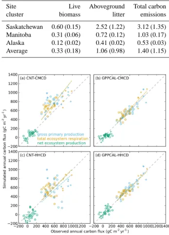
The simulated fire carbon emissions in the most recent fire events for the three site clusters for the GPPCAL-CMCD
Table 3. Simulated fire carbon emissions (kg C m−2) from live biomass, aboveground litter, and total carbon emissions for the most recent fire event for the three site clusters by GPPCAL-CMCD sim-ulation. The mean values for each site cluster are shown in the table with standard deviation being shown within brackets.
Site Live Aboveground Total carbon cluster biomass litter emissions Saskatchewan 0.60 (0.15) 2.52 (1.22) 3.12 (1.35) Manitoba 0.31 (0.06) 0.72 (0.12) 1.03 (0.17) Alaska 0.12 (0.02) 0.41 (0.02) 0.53 (0.03) Average 0.33 (0.18) 1.06 (0.98) 1.40 (1.15)
Fig. 2. Simulated vs. observed annual gross primary production (sky
blue), total ecosystem respiration (orange) and net ecosystem pro-duction (green), before (a, c) and after (b, d) nudging observed mean multi-year GPP. Observed annual carbon fluxes are from Amiro et al. (2010). A 1 : 1 line is shown as the dashed gray line. Colored dashed lines indicate RTO regression lines. Distinctions are made among Manitoba (circles), Saskatchewan (cross symbol, “+”) and Alaska (stars) data.
simulation are: for Saskatchewan 3.12 ± 1.3 kg C m−2,
for Manitoba 1.03 ± 0.17 kg C m−2, and for Alaska
0.53 ± 0.03 kg C m−2(Table 3). The mean fire-carbon
emis-sions among all the 13 study sites are 1.40 ± 1.15 kg C m−2,
with 0.33 kg C m−2 being emitted from crown burning and
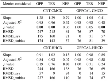
Table 4. Model-measurement comparison metrics for annual GPP,
TER and NEP. The left-hand (right-hand) column shows values be-fore (after) nudging the observed multi-year GPP into the model (see Sect. 2.4.4 for more details).
Metrics considered GPP TER NEP GPP TER NEP
CNT-CMCD GPPCAL-CMCD Slope 1.28 1.29 0.79 1.00 1.05 0.41 Adjusted R2 0.95 0.96 0.62 0.98 0.98 0.48 pvalue 0.00 0.00 0.06 1.00 0.05 0.00 RMSD 247 215 61 76 87 70 RMSD_sys 175 160 21 0 31 57 RMSD_unbias 174 143 57 76 81 39 CNT-HHCD GPPCAL-HHCD Slope 0.91 1.02 0.13 1.00 0.98 0.85 Adjusted R2 0.84 0.92 −0.02 0.98 0.98 0.58 pvalue 0.19 0.76 0.00 1.00 0.31 0.24 RMSD 244 166 138 76 76 69 RMSD_sys 57 9 84 0 14 15 RMSD_unbias 237 166 110 76 74 67
Linear regression (of form y = slope · x) is fitted between simulated and observed annual data across all evaluation sites. Sample size is 33 for GPP, and 31 for TER and NEP. Data reported here include regression slope, and the probability of the slope being significantly not different from 1 (p value), adjusted goodness of fit (adjusted R2,a modification of R2
that adjusts for the number of explanatory variables), root mean square deviation (RMSD), systematic and unbiased RMSD (see Sect. 2.5.2 for detailed description). Tests with pvalue < 0.05 (i.e., slope 6= 1) are bold for emphasis.
3.2 Evaluation of simulated annual GPP, TER and NEP
Simulated annual GPP, TER and NEP is compared to EC measurements in Fig. 2. Model outputs are shown for sim-ulations both before (CNT-CMCD and CNT-HHCD) and af-ter (GPPCAL-CMCD and GPPCAL-HHCD) multi-year av-erage GPP assimilation. Note, in the GPPCAL simulations, only the average multi-year GPP from the model is opti-mized to the measured mean value, so that the simulated inter-annual variability of GPP can still be compared to EC data.
The CNT-CMCD simulation without GPP nudging, over-estimates both GPP and TER across all study sites (Table 4, Fig. 2a) by approximately 30 %. No overestimation can be seen for NEP in CNT-CMCD simulation (Table 4, Fig. 2a), suggesting compensation of GPP and TER biases in NEP. In the CNT-HHCD simulation, the RTO regression slopes for GPP and TER are not significantly different from unity, in-dicating no systematic bias in simulation of these two car-bon fluxes. Whereas NEP in CNT-HHCD is significantly lower than measurement values (∼ 85 % by RTO slope). This shows that the choice of climate forcing data (low vs. high frequency) strongly affects the model-data misfit.
For CNT-CMCD simulation, the simulated to observed multi-year average GPP ratios are different for each of the three clusters of evaluation sites. This ratio is 1.15 ± 0.27 for Saskatchewan sites, 1.42 ± 0.17 for Manitoba sites, and 2.13 ± 0.13 for Alaska sites. The overestimate of simulated GPP tends to be larger at higher latitudes.
Fig. 3. Simulated and measured leaf area index (LAI) as a function
of time after fire. Model results (Manitoba: sky blue, Saskatchewan: green, Alaska: orange) are presented by pooling together outputs for all evaluation sites of the same cluster, with the solid line in-dicating the mean value, and shaded area showing between-site minimum–maximum range. Measurements from different sources are shown separately for Manitoba (circles), Saskatchewan (dia-monds) and Alaska (triangles), with wet (dry) site measurements as filled (open) signs. Error bars on the measurement points indicate 90 % confidence interval measurement uncertainty. The inset panel shows the overall model-measurement agreement along a 1 : 1 line for dry (small open circles) and wet (small cross symbol, “+”) site measurements separately.
Because the GPPCAL-CMCD and GPPCAL-HHCD runs use the same nudged GPP, the model-measurement met-rics for annual GPP are the same for these two simu-lations (Table 4). As expected, nudging multi-year aver-age GPP greatly improves the model-measurement agree-ment for annual GPP, with RTO regression slope equal to unity, and RMSD being reduced by more than ∼ 70 % compared to the non-assimilated runs (Table 4). Nudging GPP simultaneously improves the TER simulation in both GPPCAL-CMCD and GPPCAL-HHCD simulations. Model-measurement agreement for NEP in GPPCAL-HHCD is also improved after assimilation (RTO regression slope changes from 0.13 to 0.85, RMSD is reduced by more than half; Ta-ble 4), but NEP remains underestimated (too small a modeled carbon sink) in GPPCAL-CMCD.
3.3 Evaluation of postfire evolution of LAI, biomass, forest floor, woody debris, and mineral soil organic carbon
In this section, the evaluations of ORCHIDEE-FM-BF out-put against biometric measurements are presented for LAI, biomass carbon, forest floor carbon, woody debris and min-eral soil carbon (Table 5). Note that the two GPP calibration simulations only differ for the EC observation period and car-bon stocks are not expected to change greatly during these
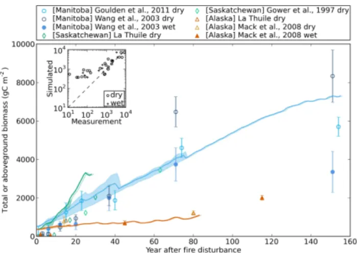
Fig. 4. Simulated vs. observed total biomass carbon (for
Man-itoba) and aboveground biomass carbon (for Saskatchewan and Alaska) as a function of time after fire. Model results (Manitoba: sky blue, Saskatchewan: green, Alaska: orange) are presented by pooling together outputs for all evaluation sites of the same clus-ter, with the solid line indicating the mean value, and shaded area showing between-site minimum–maximum range. Measurements from different sources are shown separately for Manitoba (circles), Saskatchewan (diamonds) and Alaska (triangles), with wet (dry) site measurements as filled (open) signs. Error bars on the measure-ment points indicate 90 % confidence interval measuremeasure-ment uncer-tainty. The inset panel shows the overall model-measurement agree-ment along a 1 : 1 line for dry (small open circles) and wet (small cross symbol, “+”) site measurements separately.
few years, thus the simulation results from the GPPCAL-CMCD simulation are used for comparison.
3.3.1 Leaf area index
RTO regression slope between simulated and measured LAI indicates that the model underestimates LAI by an over-all fraction of 24 % (RTO regression equal to 0.76, see Ta-ble 5) when all sites are considered together. The LAI in dry sites is underestimated by ∼ 30 % by the model and wet sites overestimated by 15 % (Table 5). The overlap ratio be-tween simulated and measured data is 0.43, indicating 43 % of measurements are well simulated by the model. A close look at the model- and measurement data shows that LAI in the Manitoba dry sites have been underestimated by 50 % in the middle-aged forest (∼ 80 yr) and by 30 % in the old-aged forest (∼ 150 yr) (Fig. 3). The underestimation in the intermediate-aged forest is partly because the whole sim-ulation pixel is prescribed to be fully covered by the bo-real needleleaf trees, and this precludes the occurrence of broadleaf trees, which often dominate the early succession stage and have higher LAI and productivity.
Fig. 5. Simulated vs. observed forest floor carbon stock as a function
of time after fire. Model results (Manitoba: sky blue, Saskatchewan: green, Alaska: orange) are presented by pooling together outputs for all evaluation sites of the same cluster, with the solid line in-dicating the mean value, and shaded area showing between-site minimum–maximum range. Measurements from different sources are shown separately for Manitoba (circles), Saskatchewan (dia-monds) and Alaska (triangles), with wet (dry) site measurements as filled (open) signs. Error bars on the measurement points indi-cate 90 % confidence interval measurement uncertainty. The inset panel shows the overall model-measurement agreement along a 1:1 line for dry (small open circles) and wet (small cross symbol, “+”) site measurements separately.
3.3.2 Total and aboveground biomass
With the re-growing of the forest stand after fire, forest biomass carbon is modeled to increase continuously with for-est age (Fig. 4). The RTO regression slope for all dry and wet sites combined is not significantly different from unity, indi-cating a very good overall model-measurement agreement. Yet for wet sites, modeled biomass carbon is overestimated by about 50 %, with a larger systematic RMSD than unbi-ased RMSD, likely because ORCHIDEE-FM-BF does not limit growth sufficiently at wet sites.
3.3.3 Forest floor carbon
RTO regression analysis indicates that forest floor carbon is underestimated by ∼ 50 %, when pooling all study sites together (Table 5), explaining the bigger systematic RMSD than unbiased RMSD. But due to the large uncertainty in the measured data (Fig. 5), the overlap ratio between simulated and measured data is 0.43, which is moderately good (43 % of the measurements are reproduced by the model).
If the three clusters of sites are examined separately, some additional biases are revealed. For the Manitoba sites, for-est floor carbon is found to be underfor-estimated by the model, mainly in very young forest (< 10 yr) and forest older than
∼70 yr. In contrast, for Saskatchewan sites the model
Table 5. Model-measurements comparison metrics for LAI, biomass carbon, forest floor carbon, total woody debris, diameter at breast
height (DBH), stand individual density, and basal area (BA) (see Table S1 for the definition of the variables; see Supplement Sect. 3 for how modeled and field observation data were matched against each other for woody debris and forest floor).
Items Drainage LAI Biomass Forest floor Woody DBH Stand individual Basal
carbon carbon debris density Area
N All 33 37 35 60 12 11 12 Dry 26 27 26 53 7 6 7 Wet 7 10 9 7 5 5 5 Slope All 0.76 1.03 0.51 0.31 0.79 1.14 0.89 Dry 0.71 0.94 0.54 0.30 0.74 1.06 0.76 Wet 1.15 1.55 0.47 0.50 0.89 1.32 1.50 pvalue All 0.00 0.69 0.00 0.00 0.06 0.54 0.43 Dry 0.00 ∗0.37 0.00 0.00 0.02 ∗0.80 0.03 Wet 0.48 0.02 0.00 0.24 0.70 0.56 0.25 Adjusted R2 All 0.78 0.86 0.59 0.34 0.85 0.72 0.80 Dry 0.79 ∗0.89 0.57 ∗0.37 ∗0.94 ∗0.81 ∗0.94 Wet 0.85 0.89 0.66 0.23 0.77 0.64 0.82 Overlap ratio All 0.43 0.38 0.43 0.43 0.50 0.27 0.33 Dry ∗0.47 ∗0.38 0.35 0.43 ∗0.57 ∗0.33 ∗0.43 Wet 0.25 0.38 0.67 – 0.40 0.20 0.20 RMSD All 1.13 1018 1884 2165 1.74 6595 8.57 Dry 1.20 ∗865 ∗1810 2199 ∗1.52 ∗5481 ∗6.87 Wet 0.86 1347 2083 1890 2.00 7723 10.50 RMSD_sys All 0.58 69 1416 1839 0.93 1292 2.08 Dry 0.74 152 1279 1933 1.25 656 5.36 Wet 0.26 965 1763 900 0.42 2401 6.05 RMSD_unbias All 0.98 1015 1242 1142 1.46 6467 8.31 Dry 0.94 851 1281 1047 0.87 5441 4.30 Wet 0.83 939 1111 1662 1.96 7340 8.58
See Sect. 2.5 for explanation for all items except N, which means the sample size. Cases with p value < 0.05 are bold for emphasis (which means regression slope is significantly different from 1). Bold RMSD_sys indicates that the value of RMSD_sys is bigger than RMSD_unbias, which means RMSD is dominated by systematic error and poor model-measurement agreement. Stars (∗) indicate a better model-measurement agreement
in dry sites than in wet sites. Woody debris includes all standing dead wood (STD), downed woody debris (DWD) and total woody debris (TWD).
although this result could well be biased by the scarcity of available measurements.
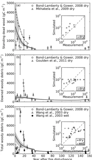
3.3.4 Woody debris
Model-measurement comparisons for woody debris, includ-ing standinclud-ing dead wood (SDW), downed woody debris (DWD) and total woody debris (TWD), are shown in Fig. 6. The RTO regression slopes between simulated and measured woody debris for dry, wet and for all sites combined are 0.31, 0.30 and 0.50 respectively, suggesting underestimation by the model. The overlap ratio is 0.43, indicating mod-erate model-measurement agreement. For dry sites and all sites combined, the systematic RMSD is bigger than unbi-ased RMSD, indicating a persistent model bias. But for wet sites, this bias is reduced and becomes smaller than unbiased RMSD.
At Manitoba sites, simulated SDW carbon is higher than field measurements for young forests (< 20 yr) (Fig. 6a). Note, for both downed woody debris and total woody de-bris, the measurements are extremely high in forests around 20 yr old. This is because tree mortality is delayed after fire
(Bond-Lamberty and Gower, 2008), whereas in the model, unburned tree biomass is considered to become standing dead wood immediately after fire.
3.3.5 Mineral soil carbon and stand structure
The simulated mineral soil carbon is compared with the ob-servation in a qualitative way. Summarizing, the simulated mineral soil carbon agrees best with the well-drained mea-surements, and is generally smaller than the poorly drained measurements. ORCHIDEE-FM-BF only has moderate to low capability at reproducing soil carbon. However the dif-ferences to observation are mainly found in the carbon pool with a small turnover rate, and thus the overall contribution to the flux error is relatively small (see Supplement Sect. 5 for more detailed discussion). The simulated forest stand in-dividual density, mean DBH and basal area generally agree well with observation (see Supplement Sect. 6 for more de-tailed description).
Fig. 6. Simulated vs. observed woody debris as a function of time
after fire for (a) standing dead wood (SDW); (b) downed woody debris (DWD); and (c) total woody debris (TWD). Data for itoba and Saskatchewan sites are shown for SDW, and only Man-itoba sites are shown for DWD and TWD. Model results are pre-sented by pooling together outputs for all the evaluation sites in the same site cluster, with the thick black (and dashed) line indicating the mean value, and shaded area showing between-site minimum– maximum range. All black lines in the three panels show the result for Manitoba sites, the dashed line in panel (a) shows the result for Saskatchewan sites. Measurements from different sources are shown for both dry (open circles and triangles) and wet (filled dots) measurements. Error bars on the measurement points indicate 90 % confidence interval measurement uncertainty. The inset panel shows the overall model-measurement agreement along a 1 : 1 line for dry (small open circles) and wet (small cross symbol, +) measurements separately.
3.4 Overall model performance across different soil drainage conditions
When examining model-measurement agreement for differ-ent soil drainage conditions, in terms of RTO regression goodness of fit (adjusted R2), overlap ratio, and RMSD, the model is found to perform better at dry sites than at wet sites
for LAI, biomass carbon stock, DBH, stand density and basal area (5 out of 6 variables for which the comparison is appli-cable). This indicates that the model has a generally better performance at dry sites than wet ones.
Model-measurement agreement metrics across all evalu-ation sites for carbon fluxes and carbon stocks are summa-rized in Table 6, together with measurement accuracy. The average model-measurement overlap ratio for LAI, biomass, forest floor and total woody debris carbon was 42 %. Except for forest floor carbon, the model-measurement RMSDs for all variables in Table 6 are lower than or equal to the uncer-tainty of field measurement, indicating that the model perfor-mance is on average satisfactory, given the uncertainty in the observed data.
3.5 Attributing the role of past climate and CO2
trends in the postfire evolution of carbon fluxes
To attribute the roles of the atmospheric CO2 and varying
climate in postfire forest CO2 fluxes trajectory, CO2
FIX-CLIMFIX and CO2FIX-CLIMVAR simulations were done
for sites CA-NS1, CA-SF1, and US-Bn1 to be compared with GPPCAL-CMCD simulations. The postfire GPP, TER and NEP trajectory for Manitoba sites are shown in Fig. 7 (see Fig. S6 for sites in Saskatchewan and Alaska). The attribu-tion analysis is done only for the period after the most recent fire events, the same period as the chronosequence study on each cluster of sites (for CA-NS1 155 yr, for CA-SF1 28 yr and for US-Bn1 83 yr).
When attributing the effects of varying CO2 and climate
for the site CA-NS1 (Manitoba), we assume that the
simu-lation result by CO2FIX-CLIMFIX for the time before 1968
(the starting year of meteorological station observations)
fol-lowed the same curve as CO2FIX-CLIMVAR. This is mainly
due to the restriction in the availability of historical climate data from the meteorological station. This assumption may lead to underestimated varying climate effects as the climate trend before 1968 is not taken into account. For clarity, we focus on the site CA-NS1 and then briefly discuss the sites CA-SF1 and US-Bn1.
We find that the temporal pattern and magnitudes of
post-fire CO2fluxes at the Manitoba sites (CA-NS1 to CA-NS7)
over the past 150 yr are greatly driven by the fertilization
effect of increasing atmospheric CO2. The EC-measured
magnitudes of postfire GPP for different ages of forest af-ter fire are much higher than the simulation result with
fixed CO2 (CO2FIX-CLIMVAR). The GPP measurements
can only be reproduced by the model if the effect of
increas-ing CO2 is accounted for (GPPCAL-CMCD, Fig. 7a). The
same also applies for TER and NEP, although the slight un-derestimation of NEP (underestimated carbon sink) by the GPPCAL-CMCD simulation is again shown (as shown in
Fig. 2c). When comparing GPPCAL-CMCD and CO2
Table 6. Model-measurement RMSD, RTO regression slope, overlap ratio for all sites combined, and measurement accuracy for GPP, TER,
NEP, LAI, biomass carbon, total woody debris and forest floor carbon.
Variable RMSD RTO regression slope Overlaping ratio Measurement Accuracy∗
Gross primary production (g C m−2yr−1) 76 – – 100
Total ecosystem respiration (g C m−2yr−1) 76 – – 200
Net ecosystem production (g C m−2yr−1) 69 – – 50
Leaf area index (m2m−2) 1.13 0.76 0.43 2
Biomass carbon (g C m−2) 1018 1.03 0.38 1000
Woody debris (g C m−2) 1885 0.35 0.43 2000
Forest floor carbon (g C m−2) 1884 0.51 0.43 1000
∗Measurement accuracy information is from Goulden et al. (2011). For GPP, TER and NEP, measurement and aggregation accuracy is used, and for other variables,
across-landscape sampling accuracy is used.
Climate effect
CO2 effect
Combined effect
Fig. 7. Simulated GPP (a), TER (b) and NEP (c) trajectory for the
time of the 20th fire rotation (since the first vertical red dashed line) and for the chronosequence period (since the second verti-cal red dashed line) for Manitoba sites. Simulation results for the scenario of varying CO2with varying climate (GPPCAL-CMCD) are shown for all seven sites in colored lines, with the scenario of fixed CO2with varying climate (CO2FIX-CLIMVA) as a gray line, and the scenario of fixed CO2 with fixed climate (CO2 FIX-CLIMFIX) as black line for the site CA-NS1. Corresponding eddy-covariance CO2flux measurements (Amiro et al., 2010; Goulden et al., 2011) at each site are shown as colored dots, with the colors corresponding to the colors of GPPCAL-simulation results for each site. For GPPCAL-CMCD simulation results, the numbers after the site names in the legend indicate the year of most recent fire event. The colored small arrows at the bottom of the panel (a) indicate the time to increase atmospheric CO2for each site in the GPPCAL-CMCD simulation.
CO2leads to both an increase in GPP and TER, and a net
increase in NEP (postfire carbon sink) (Table 7).
All three fluxes of GPP, TER and NEP are higher for the
CO2FIX-CLIMFIX simulation than CO2FIX-CLIMVAR,
in-dicating that recent climate trends alone decrease the post-fire carbon sequestration in our model simulation. GPP is decreased to a greater extent than TER when climate varies
but CO2 remains fixed, causing a net decrease in NEP
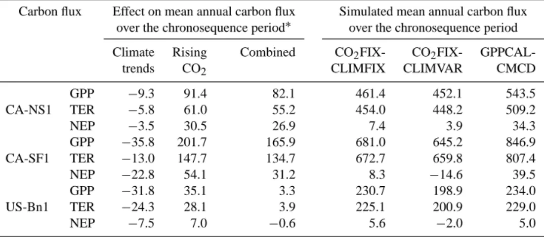
(Ta-ble 7). In summary, in terms of mean annual NEP over the entire postfire period for the site CA-NS1 (155 yr), increasing CO2caused an increase of 30.5 g C m−2yr−1in mean annual NEP but climate trends alone a decrease by 3.5 g C m−2yr−1; their combined effect is an increase of mean annual NEP by 26.9 g C m−2yr−1 (Table 7). For the period after the most
recent fire event, the GPPCAL-CMCD (varying CO2 with
varying climate) simulates a strong carbon sink in all the car-bon stock compartments (total biomass, aboveground litter, belowground litter and mineral soil organic carbon) in the forest and accumulated NEP is 4.6 times higher than the car-bon emissions in the fire (see Tables S3, S4 and S5 in the Supplement for the carbon budget for the three simulations at the three sites).
The role of varying CO2 and climate in postfire carbon
fluxes trajectory for the sites CA-SF1 and US-Bn1 is sim-ilar to that for CA-NS1. In terms of mean annual NEP over the period after the most recent fire event for
CA-SF1 (28 yr), increasing CO2 caused an increase in NEP by
54.1 g C m−2yr−1, while varying climate resulted in a de-crease by 22.8 g C m−2yr−1; their combined effect is an
increase in mean annual NEP of 31.2 g C m−2yr−1. For
US-Bn1 (83 yr), increasing CO2 caused an increase of
7.0 g C m−2yr−1in mean annual NEP while varying climate a decrease by 7.5 g C m−2yr−1, leading to a decrease in mean annual NEP of 0.6 g C m−2yr−1.
4 Discussion
In the preceding sections, the ORCHIDEE-FM-BF model is evaluated against chronosequence measurements of carbon
Table 7. Effects of varying atmospheric CO2and climate and their combined effect on mean annual carbon fluxes (g C m−2yr−1)over the chronosequence study period after the most recent fire event. The respective postfire period length for the evaluation sites CA-NS1, CA-SF1 and US-Bn1 are 155, 28 and 83 yr.
Carbon flux Effect on mean annual carbon flux Simulated mean annual carbon flux over the chronosequence period∗ over the chronosequence period Climate Rising Combined CO2FIX- CO2FIX-
GPPCAL-trends CO2 CLIMFIX CLIMVAR CMCD
CA-NS1 GPP −9.3 91.4 82.1 461.4 452.1 543.5 TER −5.8 61.0 55.2 454.0 448.2 509.2 NEP −3.5 30.5 26.9 7.4 3.9 34.3 CA-SF1 GPP −35.8 201.7 165.9 681.0 645.2 846.9 TER −13.0 147.7 134.7 672.7 659.8 807.4 NEP −22.8 54.1 31.2 8.3 −14.6 39.5 US-Bn1 GPP −31.8 35.1 3.3 230.7 198.9 234.0 TER −24.3 28.1 3.9 225.1 200.9 229.0 NEP −7.5 7.0 −0.6 5.6 −2.0 5.0
∗Climate effect was calculated as difference between simulations of CO
2FIX-CLIMVAR and CO2FIX-CLIMFIX, and CO2effect was calculated as difference between simulations of GPPCAL-CMCD and CO2FIX-CLIMVAR, and combined effect as difference between simulations of GPPCAL-CMCD and CO2FIX-CLIMFIX.
fluxes, ecosystem carbon pools and stand structure, with fo-cus on the capability of the model to reproduce the tempo-ral evolution of each variable as a function of time-after-fire. To our knowledge, this is the first study that tries to evalu-ate a global process-based vegetation model for fire distur-bances against multiple sites and multiple observation data sets. Although we believe the chronosequence stands are usu-ally carefully selected to make them comparable and thus represent the process of forest development, there are still site-specific conditions which lead to spatial heterogeneity among sites and complicate model-measurement compari-son. So the discussion below will focus on the more general issues on model-measurement comparison rather than ex-plaining why some specific site or variable is overestimated or underestimated by the model.
4.1 Effect of nudging observed multi-annual average GPP on improving other CO2fluxes
As shown in Sect. 3.2, nudging observed GPP has improved the model-measurement agreement for carbon fluxes. Be-sides, the RMSDs for the carbon pool and stand structure variables have been reduced by 1–40 % in the GPPCAL-CMCD simulation compared with CNT-GPPCAL-CMCD simulations (RMSDs for CNT-CMCD simulations not shown).
The GPPCAL-HHCD simulation has better agreement with observation in terms of TER and NEP than the GPPCAL-CMCD simulation. This is because the 30 min climate fields used in the GPPCAL-HHCD simulation are assumed to be more realistic than the monthly ones in the GPPCAL-CMCD simulation. This forcing-related model output bias could not be completely solved by model
calibra-tion, which has also been noticed by Zhao et al. (2012) and Lin et al. (2011).
4.2 Fire carbon emissions
The simulated fire carbon emissions are highest at Saskatchewan sites and lowest at Alaskan sites. As the fire combustion fraction is fixed in the model, the amount of sim-ulated carbon emissions is directly related to the simsim-ulated forest floor carbon stock, which is the major source of the carbon emissions in boreal fires.
In a synthesis study of fire carbon emissions in North America, French et al. (2011) reported higher average
car-bon emissions in Alaska (2–5 kg C m−2) than in Canadian
fires (1.2–1.9 kg C m−2), probably due to a higher level of organic soil carbon and deeper burning in Alaskan forests. Our simulated average fire carbon emissions for the Mani-toba and Saskatchewan sites are 1.65 kg C m−2and are there-fore within the range given by French et al. (2011). However, the simulated emissions at Alaskan sites (0.53 kg C m−2)are far below their reported value, and are also lower than those
reported by Randerson et al. (2006, 1.56 kg C m−2 for the
site US-Bn3), and Kasischke and Hoy (2012, 3.01 kg C m−2
during large fire years and 1.69 kg C m−2 during small fire years).
The underestimation of fire carbon emissions at Alaskan sites could be partly explained by the underestimation in for-est floor carbon stock. The forfor-est floor carbon stock is
under-estimated by ∼ 60 % (simulated ∼ 1.3 kg C m−2vs. observed
∼3.3 kg C m−2). Correspondingly, fire carbon emissions are
underestimated by 65–80 % (simulated 0.5 kg C m−2vs.
re-ported 1.5–3 kg C m−2from local studies). Besides, the sim-ple combustion fraction scheme used in the model does not
allow combustion fraction to vary with fire conditions, and this might also contribute to the errors in carbon emission estimation, as several studies point out that surface fuel com-bustion fraction contributes to the biggest uncertainty in esti-mating fire carbon emissions from boreal forest fires (French et al., 2004; de Groot et al., 2009).
4.3 Model performance across different soil drainage conditions
One characteristic of boreal forest ecosystems is that ecosys-tem processes are greatly modulated by soil drainage con-ditions (Wang et al., 2003; Bond-Lamberty et al., 2006). Well-drained stands occur on flat upland or south-facing slopes and are often not underlain by permafrost. Poorly drained stands occur on flat lowland, or north-facing slopes and are generally underlain by continuous or discontinuous permafrost (Harden et al., 1997, 2001; Wang et al., 2003; Turetsky et al., 2011). Stands with poor soil drainage are of-ten found to be associated with open canopy forests with relatively poor tree growth and a low biomass, abundant bryophyte layer such as sphagnum (Sphagnum spp.) which typically grows in wet environments (Wang et al., 2003), fre-quently flooded soil, and a massive amount of organic soil carbon due to the slow decomposition in the anaerobic envi-ronment (Bond-Lamberty et al., 2006).
ORCHIDEE-FM-BF is found to perform better in well-drained sites than in poorly well-drained ones. This is an ex-pected result which could be explained by several key pro-cesses in the model. First, the soil hydrological propro-cesses in ORCHIDEE-FM-BF are simulated in a way that allows soil water to drain away as runoff or infiltration when exces-sive precipitation occurs (Ducoudré et al., 1993), this proce-dure does not allow soil flooding. In reality, soils on poorly drained sites (either underlain by permafrost or due to to-pographic effects) tend to be saturated with water. In addi-tion, the thick surface organic layer acts to maintain mois-ture (Harden et al., 2006). These processes are however not included in ORCHIDEE-FM-BF. Second, in current versions of ORCHIDEE, the soil moisture always has a positive ef-fect on photosynthesis (Krinner et al., 2005); the model fails to represent the detrimental effect of excessive soil water on plant roots and the negative effect on photosynthesis.
To improve model performance on poorly drained sites of a general process biogeochemical model such as OR-CHIDEE, the poor drainage related hydrological and eco-physiological processes need to be incorporated into the model. These processes may include, for example, frequent soil flooding, detrimental effects of excessive soil water on root function and photosynthesis (Kreuzwieser et al., 2004), and reduced soil organic matter decomposition and nutrient mineralization (Wickland and Neff, 2007) in case of exces-sive soil moisture. Despite some valuable attempts (Bond-Lamberty et al., 2007a; Pietsch et al., 2003; Yi et al., 2010), the explicit process-based representation of a forest with poor
soil drainage or forested wetlands or peatland remains a big challenge in general process biogeochemical models.
Nevertheless, to examine the potential errors for regional application of ORCHIDEE-FM-BF on carbon fluxes and biomass carbon stocks, we tried to upscale the site-level sim-ulation errors from both good and poor drainage conditions (Table 5) to regional scale, by using the soil drainage dis-tribution information in both Alaska and Canada. The soil drainage map for Alaska by Harden et al. (2001) shows that
∼60 % of the soils were drained to moderately
well-drained. For Canada, 65–75 % of the soils are well-drained or moderately well-drained (Soil Landscapes of Canada Work-ing Group, 2010). To upscale the site-level error to regional scale in a rather simple way, the RTO regression slopes for dry and wet sites (Table 5) were used together with dry/wet soil distribution to derive an area-weighted error. Using this method, the model will probably generate an overestimation of total/aboveground biomass carbon stock by 12 % (Canada) to 18 % (Alaska), which is still within or comparable to the uncertainty of inventory-based net land–atmosphere carbon fluxes at national (Stinson et al., 2011) or regional scales (Hayes et al., 2012).
In summary, the model performance is found to be gen-erally acceptable if all dry and wet sites are considered to-gether. A process-based generic model like ORCHIDEE-FM-BF should not be fine-tuned at each study site for fur-ther reducing each error. Contrarily, only a multi-site agree-ment can be expected to assess for instance the model’s ca-pability to make regional simulations. Based on the results in Table 6, the key information is that the model-measurement error across multiple sites is comparable with the measure-ment accuracy, which justifies using the model for regional applications.
4.4 The role of past climate and CO2trends in the
postfire evolution of carbon fluxes
4.4.1 The role of increasing atmospheric CO2
We find a significantly positive role of increasing
atmo-spheric CO2in explaining the postfire carbon uptake as
ob-served by the chronosequence method. Other studies also re-port similar positive effects of historical CO2in increasing the boreal regional carbon stock (Balshi et al., 2007; Hayes et al., 2011). This is reasonable as the ambient CO2 concen-tration is one of the factors that limit plant photosynthetic activity (Chapin III et al., 2002).
Our results also reveal some more interesting aspects of
the CO2 fertilization effect on plant carbon uptake in the
context of forest succession. As shown in Fig. 7, the mag-nitude of postfire GPP on each site, as measured by the chronosequence method, could only be reproduced at exactly the same simulated site, but not at others (for easy identifica-tion, the simulation data for the GPPCAL-CMCD simulation and measurement data for a single site are plotted in the same