HAL Id: hal-01179489
https://hal.inria.fr/hal-01179489
Preprint submitted on 22 Jul 2015
HAL is a multi-disciplinary open access
archive for the deposit and dissemination of
sci-entific research documents, whether they are
pub-lished or not. The documents may come from
teaching and research institutions in France or
abroad, or from public or private research centers.
L’archive ouverte pluridisciplinaire HAL, est
destinée au dépôt et à la diffusion de documents
scientifiques de niveau recherche, publiés ou non,
émanant des établissements d’enseignement et de
recherche français ou étrangers, des laboratoires
publics ou privés.
On the Scalability of Constraint Solving for
Static/Off-Line Real-Time Scheduling
Raul Gorcitz, Emilien Kofman, Thomas Carle, Dumitru Potop-Butucaru,
Robert de Simone
To cite this version:
Raul Gorcitz, Emilien Kofman, Thomas Carle, Dumitru Potop-Butucaru, Robert de Simone. On the
Scalability of Constraint Solving for Static/Off-Line Real-Time Scheduling. 2015. �hal-01179489�
On the Scalability of Constraint Solving for
Static/Off-Line Real-Time Scheduling
Raul Gorcitz2, Emilien Kofman1,4, Thomas Carle3, Dumitru Potop-Butucaru1,
and Robert de Simone1
1
INRIA, France
2
CNES, France
3 Brown University, USA 4
CNRS/UNS, France?
Abstract. Recent papers have reported on successful application of con-straint solving techniques to off-line real-time scheduling problems, with realistic size and complexity. Success allegedly came for two reasons: ma-jor recent advances in solvers efficiency and use of optimized, problem-specific constraint representations. Our current objective is to assess further the range of applicability and the scalability of such constraint solving techniques based on a more general and agnostic evaluation cam-paign. For this, we have considered a large number of synthetic scheduling problems and a few real-life ones, and attempted to solve them using 3 state-of-the-art solvers, namely CPLEX, Yices2, and MiniZinc/G12. Our findings were that, for all problems considered, constraint solving does scale to a certain limit, then diverges rapidly. This limit greatly depends on the specificity of the scheduling problem type. All experimental data (synthetic task systems, SMT/ILP models) are provided so as to allow experimental reproducibility.
Keywords: real-time scheduling, satisfiability modulo theories, constraint solv-ing, repeatable
1
Introduction
Multi-processor scheduling is a vast, difficult and still open topic. It is addressed in several research areas (real-time scheduling, parallel compilation,. . . ), using various formal resolution approaches (from operations research to dedicated al-gorithmics). Still, regardless of the area or the solving approach, the majority of multiprocessor scheduling problems are NP-hard [7, 14]. Only a few utterly simple cases have polynomial solutions [5].
While NP-hard complexity is usually bad news, because some medium-size problem instances may be found to be intractable, it is not always so. And,
?This work was partly funded by the French Government (National Research Agency,
ANR) through the Labex UCN@sophia (“Investments for the Future” Program #ANR-11-LABX-0031-01), and the HOPE project (#ANR-12-INSE-0003).
because of the regularity induced by human-made specifications, the tough com-plexity sometimes only occur in accidental pathological descriptions. In fact, many instances of NP-hard problems can be rapidly solved in practice using exact algorithms [10]. This led to a renewal of interest in the improvement of solvers to increase their efficiency, a topic once thought as almost closed decades ago. And these recent improvements in solver power in turn led researchers for a renewed interest in using these exact techniques for solving problems such as multi-processor scheduling (whose need in part motivated the solver’s improve-ments, so that everything gets quite intricated in the end).
Another avenue of research in this area was (and still is) the definition of in-sightful heuristics for fast scheduling, with generally admittedly good results. We shall not consider heuristic approaches here, partly because they are by defini-tion non-optimal (meaning that they have no guarantee to find a schedule when one exists, or that their solution is close or not to being optimal), but mostly because the current relevance of exact scheduling techniques relying on top-class constraint solvers is our actual research concern in this paper. It is therefore always interesting to determine when exact/optimal techniques work. This is exactly our objective here: to determine the limits of applicability of exact solv-ing techniques for various multi-processor schedulsolv-ing problems. In other terms, we seek to determine the empirical practical complexity [10] of such problems.
Our approach considers static (off-line) real-time multi-processor schedul-ing problems, encoded as specifications made for satisfiability modulo theories (SMT), integer linear programming (ILP), or more general constraint program-ming (CP). The encodings themselves cover a range of scheduler features: single-period vs. multi-single-period, non-preemptive vs. preemptive, non-dependent vs. de-pendent tasks, heterogenous architectures vs. homogenous architectures, schedu-lability verification vs. optimization. For each scheduling problem we study the evolution of resolution time as number of tasks and processors grow, under dif-ferent system loads. We deduce in a systematic way for which range of values exact constraint resolution can be applied within reasonable time, and where are the actual limits of tools and methods.
The problem instances we consider include (mostly) synthetic and (a few) real-life examples. Constraints are generated from tasks graphs in a systematic way [6]. Tasks graphs are usually displaying some amount of parametric sym-metry which allows us to produce even more constraints [13] (see Section 4.2). This allows to select one solution out of a stable symetric class and thus cuts down the search space complexity.
We solve the resulting specifications using 3 state-of-the-art solvers: CPLEX for ILP specifications, Yices2 for SMT, and MiniZinc/G12 for the CP programs. We thus determine the (average) time required to solve instances of the schedul-ing problems for each type of problem and for each choice of parameters (number of tasks/processors and system load).
Our results indicate that, for most problems we considered, exact resolution works very efficiently for small to medium-size instances, but an abrupt combi-natorial explosion systematically occurs at some point. It is thus interesting to
figure what is the range of values for which the exact solution scales up. The limit largely depends on the particular scheduling features as described above, and on the system load (from less than 20 tasks for the optimal scheduling of average-load dependent tasks to more than 150 tasks in the schedulability analysis of single-period non-dependent, non-preemptive task systems with low system load).
By exploring the applicability limits of exact solving over multiple classes of scheduling problems, we provide insight into which characteristics of a scheduling problem make it more or less difficult to solve in practice. For instance, our results show that it is generally easier to build schedules when system utilization is low or, on the opposite, to prove unsatisfiability when load is very high.
Our experimental setting can be seen as a real-life effort at reconciling the seemingly contradictory conclusions found in two series of papers:
– Papers recording unsuccessful previous attempts at using exact techniques for off-line real time scheduling, such as [8]. This pessimistic view has recently been reinforced by evidences that it is still unfeasible to map relatively simple parallelized applications onto many-cores (cf. Section 5) or to map complex embedded control applications modeled as real-time dependent task systems onto bus-based multiprocessors when both allocation and scheduling must be computed [4]. We do not consider in this category the many other papers which discard exact solving techniques based on theoretical considerations, rather than experimental ones, because the issue is indeed to consider the potential gap between the two.
– A few recent papers reporting the successful application of modern constraint solving tools to realistic real-time scheduling and compilation problems[12, 6], due to increase in solver efficiency.
As suggested by our experiments, the brute-force application of exact meth-ods to any-size problems shall certainly comfort the first point-of-view (generally the one shared amongst the real-time scheduling and compilation communities). But, still, if one gets conscious of the boundaries as well as of the care and attention that must be taken in modeling the problems to be presented to the solvers, there is now a growing range of applications that can indeed fall into the scope of these methods. And this includes already a number of problems of practical relevance, especially those displaying certain features such as low sys-tem utilization, non-preemptive execution model, few dependencies,. . . as shown in our results.
Outline The remainder of the paper is structured as follows. Section 2 reviews related work. Section 3 fully defines the ILP/SMT/CP encoding schemes used on the various scheduling problems we cover. Section 4 details the composition of our testbench, i.e. the generation rules for the synthetic examples and the structure of the non-synthetic ones. Section 5 provides and interprets the results, and Section 6 concludes.
2
Related work
One major inspiration came from previous work by Leyton-Brown et al. [10] on understanding the empirical hardness of NP-complete problems, and in particu-lar SAT. Their paper points out that SAT solving is simple(r) when either the number of constraints per variable is low (thus allowing the rapid construction of a solution) or when it is high, in which case unsatisfiability can be rapidly deter-mined. Our paper provides a similar conclusion when the number of constraints per variable is replaced with the average real-time system load. Our paper also provides a more practical evaluation of when exact solving is usable, through criteria such as solving time and timeout ratio.
Our paper also develops over previous work on applying exact solving tech-niques (ILP/SMT/CP, more classical branch-and-cut, model checking) to off-line real-time scheduling problems [12, 6, 8]. These previous results all focus on either the (improved) modeling of a given scheduling problem or on the improvement of the solver algorithm. Our objective was quite different: to evaluate the lim-its of applicability of existing techniques and to determine global patterns that hold for all scheduling problems, and which should guide the search for efficient solutions in particular cases.
Previous work also exhibits handcrafted operations research backtracking algorithms for specific scheduling problems [2] with finely tuned branching and constraint propagation policies. Our work assumes a more generic approach and uses the policies of the solvers. Depending on the tool it is sometimes possible to guide the solver in order to change those policies. Because of the variety of the studied models and tools we did not investigate those possible optimizations.
Our paper is not directly related to previous work on heuristic solving of scheduling problems. This includes work on the heuristic use of exact solving methods, such as the use of intermediate non-optimal solutions provided by op-timizaton tools, or the use of exact techniques to separately solve parts of a scheduling problem (e.g. communications scheduling). However, our work sug-gests that solving complex scheduling problems is likely to require heuristics for some time, especially given the trend of considering larger systems and adding more and more detail (non-functional requirements).
Finally, in the SMT/ILP/CP modeling of this paper we have neglected the modeling approach associated with fluid scheduling [11]. While this modeling technique bears a promise of reduced complexity, it is not clear yet whether it can deal with dependent tasks, which we consider central for the future of real-time scheduling.
3
ILP/SMT/CP modeling of scheduling problems
This section formally introduces the scheduling problems we consider and then formally defines the encodings as SMT/ILP/CP constraint systems. We consider scheduling problems of two main types: schedulability verification and optimiza-tion. Schedulability verification consists here in determining if a schedule exists
when the periods and durations of the various tasks are fixed. All optimization problems we consider concern single-period task systems. There, the objective is to compute the smallest period ensuring the existence of a schedule. Only the durations of the tasks are an input to the optimization problems. In all cases, deadlines are implicit (equal to the periods). Among the 3 solvers we use, CPLEX and MiniZinc/G12 can natively solve optimization problems, whereas Yices2 cannot.
As a baseline, we employ for all problems classical encodings, similar to the one of [6]. In the case of parallelized code running on homogenous architectures, this encoding is enriched with state-of-the-art symmetry-breaking constraints [13] that largely reduce solving time. The symmetry-breaking constraints are introduced later, in Section 4.2, after an application example has been introduced (to allow intuitive presentation).
Our encoding will assume that all time values used in the definition of the scheduling problem are a multiple of a given time base. This must hold for problem inputs, like the worst-case durations of tasks, and also for problem results (computed start dates and, for optimization problems, the period). All these time values are represented using integer constants and variables.
We directly present here only the SMT/CP encoding of the problems. The ILP encoding requires representing the Boolean logic parts of the rules with integer linear constraints. This straightforward translation is not detailed here.
3.1 Single-period dependent tasks, heterogenous architecture The first problem we consider is that of non-preemptive distributed scheduling of a set of dependent tasks having all the same period on a heterogenous set of processors connected using a single broadcast bus. The abstract formal definition of such a scheduling problem, known as a task model, must provide the following objects:
– The sets of tasks, task dependencies, and processors, respectively denoted with T, D, and P. We assume that each dependecy d ∈ D connects exactly one source task denoted Src(d) and one destination task denoted Dst(d). The elements of the task and dependency sets are ordered, so that we can write τ1> τ2 or d1< d2.
– For each τ ∈ T and p ∈ P, CanExec(τ, p) is a Boolean defining whether processor p can execute task τ . Whenever CanExec(τ, p) is true, the value WCET(τ, p) is defined as a safe upper bound of the worst-case execution time of τ on p. WCET(τ, p) is a finite integer positive value.
– For each d ∈ D, WCCT(d) is a safe upper bound of the worst-case duration of transmitting over the bus the data communication associated with d. WCCT(d) is always a positive value. We make the assumption that the bus can perform data communications associated with any d.
– Alloc(τ, p) is a Boolean variable. It is true when task τ is allocated on pro-cessor p. It is only defined and used in constraints when CanExec(τ, p) is true.
– BusAlloc(d) is a Boolean variable. It is true when a bus communication is allocated for dependency d. It must be true when the source and destination tasks of d are allocated on different processors.
– Before(τ1, τ2) is a Boolean variable. If true, it requires that task τ1is
sched-uled before task τ2, in which case τ2starts after τ1 ends.
– Before(d1, d2) is a Boolean variable. It is true when the bus communication
of dependency d1is scheduled before the communication of d2, in which case
we will require that whenever both communications are scheduled on the bus, d2 starts after d1 ends.
– Start (τ ) and Start (d) are non-negative integers providing respectively the start dates of task τ (on a processor) and communication associated with dependency d (on the bus). The value of Start (d) should only be used when BusAlloc(d) is true.
– T is the length of the schedule table, which gives the maximum period of the resulting schedule. It can be either an input of the problem, when the period is fixed, or an output, for optimization problems.
SMT/CP encoding: Constraints. The 8 following rules are used as constraint constructors for both optimization and schedulability problems. Note that con-sidering only rules [1], [2], [3], and [8] corresponds to encoding of single-period, non-dependent tasks.
[1] Each task is allocated on exactly one processor.
for all τ ∈ T do P
p∈P CanExec(τ,p)=true
Alloc(τ, p) = 1
[2] If two tasks are ordered, the second starts after the first ends.
for all p ∈ P do
for all (τ1, τ2) ∈ T2 with CanExec(τ1, p) = true and τ16= τ2 do
Before(τ1, τ2) ∧ Alloc(τ1, p) ⇒ Start (τ1) + WCET(τ1, p) ≤ Start (τ2)
[3] If two tasks are allocated on the same processor, they must be ordered.
for all p ∈ P do
for all τ1, τ2 ∈ T with CanExec(τi, p) = true, i = 1, 2 and τ1< τ2 do
Alloc(τ1, p) ∧ Alloc(τ2, p) ⇒ Before(τ1, τ2) ∨ Before(τ2, τ1)
[4] The source and destination of a dependency must be ordered.
for all d ∈ D do
Before(Src(d), Dst(d)) ∧ ¬Before(Dst(d), Src(d))
[5] The bus communication associated with a dependency (if any) must start af-ter the source task ends and must end before the destination task starts.
for all (d, p) ∈ D×P do
if CanExec(Src(d), p) = true then if CanExec(Dst(d), p) = true then
Alloc(Src(d), p) ∧ ¬Alloc(Dst(d), p) ⇒ Start (Src(d)) + WCET(Src(d), p) ≤ Start (d)
Alloc(Src(d), p) ∧ ¬Alloc(Dst(d), p) ⇒ Start (d) + WCCT(d) ≤ Start (Dst(d)) Alloc(Src(d), p) ∧ ¬Alloc(Dst(d), p) ⇒ BusAlloc(d)
else
Alloc(Src(d), p) ⇒ Start (Src(d)) + WCET(Src(d), p) ≤ Start (d) Alloc(Src(d), p) ⇒ Start (d) + WCCT(d) ≤ Start (Dst(d)) Alloc(Src(d), p) ⇒ BusAlloc(d)
[6] When two dependencies require both a bus communication, these communi-cations must be ordered.
for all (d1, d2) ∈ D2with d1< d2 do
BusAlloc(d1) ∧ BusAlloc(d2) ⇒ Before(d1, d2) ∨ Before(d2, d1)
[7] If two dependencies are ordered, the first must end before the second starts.
for all (d1, d2) ∈ D2with d16= d2 do
Before(d1, d2) ⇒ Start (d1) + WCCT(d1) ≤ Start (d2)
[8] All tasks must end at a date smaller or equal than the schedule length.
for all (p, τ ) ∈ P×T with CanExec(τ, p) = true do
Alloc(τ, p) ⇒ Start (τ ) + WCET(τ, p) ≤ T
3.2 Simplified encoding for the homogenous case
In the homogenous case, all processors have the same computing power, so that for each task τ we only need to define a single duration WCET(τ ). We still allow some allocation constraints: A task τ has either fixed allocation, in which case CanExec(τ, p) is true for exactly one of the processors p, or can be executed on all processors, in which case CanExec(τ, p) is true for all p. The constraint rules [2], [5], and [8] need to be replaced with the following simplified rules.
[2hom] If two tasks are ordered, the second starts after the first ends.
for all p ∈ P do
for all (τ1, τ2) ∈ T2 with CanExec(τ1, p) = true and τ16= τ2 do
Before(τ1, τ2) ∧ Alloc(τ1, p) ⇒
Start (τ1) + WCET(τ1) ≤ Start (τ2)
[5hom] The bus communication associated with a dependency (if any) must start after the source task ends and must end before the destination task starts.
for all (d, p) ∈ D × P do
if CanExec(Src(d), p) = true then if CanExec(Dst(d), p) = true then
Alloc(Src(d), p)∧¬Alloc(Dst(d), p) ⇒ Start (Src(d))+WCET(Src(d)) ≤ Start (d) Alloc(Src(d), p) ∧ ¬Alloc(Dst(d), p) ⇒ Start (d) + WCCT(d) ≤ Start (Dst(d)) Alloc(Src(d), p) ∧ ¬Alloc(Dst(d), p) ⇒ BusAlloc(d)
else
Alloc(Src(d), p) ⇒ Start (Src(d)) + WCET(Src(d)) ≤ Start (d) Alloc(Src(d), p) ⇒ Start (d) + WCCT(d) ≤ Start (Dst(d)) Alloc(Src(d), p) ⇒ BusAlloc(d)
[8hom] All tasks have release date 0 and implicit deadline (equal to the pe-riod), so that they must end at a date smaller or equal than the schedule length.
Start (τ ) + WCET(τ ) ≤ T
3.3 Multi-period, non-preemptive, non-dependent tasks
The scheduling problem has now a new input: For each task τ ∈ T, we define its period, denoted T(τ ). It must be a positive integer. Unlike in the single-period case, we shall not require here that all tasks have release date 0. The deadline of each task is equal to its period.
We provide here only the encoding for the heterogenous architecture case. The homogenous case can be easily derived. The encoding uses the same variables as for single-period tasks. To account for the multi-period case, the upper bound for Start (τ ) is set to T(τ )−1 for all τ . Among the constraints, we use unmodified rule [1]. Rules [4]-[7] are not used here, because we have no dependencies. Rule [8] is no longer needed because tasks do not have release date 0. Rules [2] and [3] are replaced by a single rule (LCM denotes here the least common multiple of two integers):
[2mpnp] Instances of two different tasks cannot overlap.
for all (p, τ1, τ2) ∈ P × T × T with CanExec(τi, p) = true, i = 1, 2 and τ1< τ2 do
for all −1 ≤ α < LCM(T(τ1), T(τ2))/T(τ1) do
for all −1 ≤ β < LCM(T(τ1), T(τ2))/T(τ2) do
Alloc(τ1, p) ∧ Alloc(τ1, p) ⇒
(Start (τ1) + α ∗ T(τ1) + WCET(τ1, p) ≤ Start (τ2) + β ∗ T(τ2))∨
(Start (τ2) + β ∗ T(τ2) + WCET(τ2, p) ≤ Start (τ1) + α ∗ T(τ1))
3.4 Multi-period, preemptive, non-dependent tasks
In the preemptive model, a task can be interrupted and resumed. In our off-line scheduling context, the date of all interruptions and resumptions is an output of the scheduling problem. These dates are taken in the same integer time base as the start dates, periods... For simplicity, we consider non-dependent tasks, and we only provide here the encoding for heterogenous architectures. Preemption costs are neglected (as often in real-time scheduling). Migrations are not allowed. The encoding basically replaces each preemptable task with a sequence of non-preemptable tasks of duration 1 which must be all allocated on the same processor. The output of the scheduling problem consists in one start date for each unit task. We denote with Start (τ, p, i) the start of the ith unit task of task τ on processor p, where i ranges from 0 to WCET(τ, p) − 1. The bounds for Start (τ, p, i) are the same as for Start (τ ) in the non-preemptive multi-period case. Among the constraints, we preserve unchanged only rule [1]. Rules [4]-[8] are not needed (as explained for the non-preemptive case). Rules [2] and [3] are modified as follows:
[2mpp] Unit task instances of different tasks do not overlap.
for all (p, τ1, τ2) ∈ P × T2 with CanExec(τ1, p) and CanExec(τ2, p) and τ1< τ2 do
for all 0 ≤ α < LCM(T(τ1), T(τ2))/T(τ1) do
for all 0 ≤ β < LCM(T(τ1), T(τ2))/T(τ2) do
Alloc(τ1, p) ∧ Alloc(τ1, p) ⇒
Start (τ1, p, i) + α ∗ T(τ1) 6= Start (τ2, p, j) + β ∗ T(τ2)
[3mpp] Multiple reservations made for a given task cannot overlap.
for all (p, τ ) ∈ P × T with CanExec(τ, p) = true do for all 0 ≤ i < WCET(τ, p) − 1 do
Start (τ, p, i) < Start (τ, p, i + 1)
4
Test cases
As often in real-time scheduling, we perform measurements on large numbers of synthetic test cases. In addition, we consider two real-life signal processing applications (an implementation of the Fast Fourier Transform, and an automo-tive platooning application), typical for the field of real-time implementation of data-parallel applications.
4.1 Test case generation
Synthesizing test cases posed significant challenges, because we must allow for meaningful comparisons between a variety of scheduling problems. For instance, we could not use the state-of-the-art algorithm UUniFast [3] because it does not cover heterogenous architectures. Finally, we decided to use two synthesis algorithms.
The first one, used in comparisons involving non-dependent tasks, can be seen as an extension of UScaling [3]. For each type of scheduling problem and choice of system load, we generate examples with number of taks n ranging from 7 to 147 tasks, with an increment of 5. For each task size, we generate 40 problem instances (reduced to 25 instances for the more complex multiperiodic preemp-tive case). For each instance of a multi-period problem, periods are randomly assigned to the tasks uniformly in the set {5, 10, 15, 20, 30, 60}. For single-period schedulability problems, the period of all tasks is set to 60. In all cases, the number of processors is set to dn/5e.
The choice of system load is done by setting the maximal per-task processor usage value u. For a task τ of period T(τ ), WCET values are chosen randomly, with a uniform distribution, in the interval [1..bu ∗ T(τ )c]. For single-period op-timization problems T(τ ) is replaced in the formula by 60 for all tasks. Our measurements will use values of u ranging in the set {0.1, 0.3, 0.35, 0.5}. Given the way the number of processors is computed, this respectively corresponds to average system loads of approximately 25%, 75%, 87.5%, and 125%.
Each task is designated, with a 30% probability, a fixed-allocation task. In this case, a processor is randomly allocated to it (with uniform distribution), and a WCET value is only assigned for the task on this processor. In the heterogenous case, for each task τ that does not have fixed allocation, and for each processor p, we decide with 70% probability that τ can be executed on p, in which case we generate WCET(τ, p) as explained above.
The second generation algorithm is used in the comparison involving single-period dependent task systems. We use here the algorithm proposed by Carle and Potop [4] (in section 6). We use this algorithm to synthesize a single set of 40 random test cases. For each of these examples we create one SMT system including the dependence-related constraints, and one without these constraints.
4.2 Signal processing case studies
FFT. The first application is a parallelized version of the Cooley-Tukey imple-mentation of the integer 1D radix 2 FFT [1]. The FFT has a recursive nature, as the task graph of the FFT on 2n+1inputs is obtained by instantiating twice the
FFT on 2n inputs and then adding 2n tasks. For instance, the task graph of an
8-input FFT, provided in Fig. 1(middle) can be obtained by instantiating twice the task graph of the 4-input FFT, and then adding the 4 tasks of the bottom row. In each of the 3 task graphs of Fig. 1, nodes are tasks and arcs are data dependencies. All dependencies in an FFT transmit the same amount of data.
r00 r11 r01 r10 r02 r32 r11 r22 r31 r12 r20 r01 r00 r21 r10 r30 r02 r03 r43 r23 r00 r41 r01 r60 r71 r31 r50 r21 r61 r62 r73 r33 r32 r72 r12 r22 r53 r13 r51 r20 r11 r52 r42 r70 r30 r63 r40 r10
Fig. 1: From left to right: FFT task graphs for 4, 8 and 16 inputs
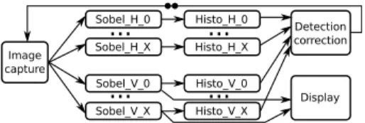
Platooning. This application is run by one car in order to automatically follow the car in front of it. It takes input from an embedded camera and controls the speed and steering of the car. It uses a Sober filter and a histogram search in order to detect the front car in the captured images. The detection and correction function uses this data to correct car speed and steering. It also adjusts image capture parameters, which creates a feedback loop in the model. The feedback dependency arc initially contains 2 tokens.
Image capture Detection correction Display Sobel_V_0 Sobel_V_X
...
Histo_V_0 Histo_V_X...
Sobel_H_0 Sobel_H_X...
Histo_H_0 Histo_H_X...
The image processing part of the application can be parallelized, by splitting the image into regions which can be processed independently. The task graph of the application (after parallelization) is provided in Fig. 2. The parallelism (of split/merge type) can be raised or decreased by changing the value of X. This means that the application exibhits both task parallelism (breadth) and pipeline parallelism (depth).
Encoding of the examples and symmetry breaking The task graphs of the 2 examples are transformed into a set of constraints by assuming that imple-mentation is done on 3 homogenous processors connected by a bus, according to the rules of Section 3.2. But our examples feature multiple identical processors and split/merge parallelism defining groups of identical tasks [13]. Thus, the re-sulting SMT/CP encoding is not very efficient, a solver being forced to spend a lot of time traversing many equivalent configurations that are identical up to a permutation of identical tasks or processors. This can be avoided by adding symmetry-breaking constraints to the initial constraint system.
In mapping the platooning application, a solver will explore the configura-tions where task Sobel H 0 starts before Sobel H 1, but also those where So-bel H 1 starts before SoSo-bel H 0. However these two tasks have symmetric de-pendencies and have the same cost so that exploring only one of the cases is enough to solve the constraint system. This also means that one can swap them (and their Histo dependency) without violating any dependency and without modyfing the resulting makespan. Formally, if Ts is a set of symmetric tasks in
T (as defined in [13]), then we add to the constraint system the following rule: [9] Start dates of symmetric tasks are ordered.
for all (τ1, τ2) ∈ Ts2 with τ1< τ2do
Start (τ1) ≤ Start (τ2)
As like as task symmetries, core symmetries can be exploited by constraining the allocation of tasks to processors, as explained in [13].
5
Experimental results
We have run the SMT/ILP/CP specifications of the previous section respectively through the Yices 2, CPLEX, and MiniZinc/G12 solvers on 8-core Intel Xeon workstations. Solving was subject to a timeout of 3600 seconds (1 hour) for synthetic test cases and 1800 seconds for the FFT and platooning applications. For all synthetic schedulability problems we have used both Yices 2 and CPLEX. Scalability findings are similar for the two solvers,5 so we will always plot only one of the result sets. Comparisons are only made between figures obtained using the same solver. For the FFT and platooning applications we have used MiniZinc/G12.
5
We found differences between solvers, but they do not affect scalability and for space reasons we cannot present them here.
5.1 Synthetic test cases
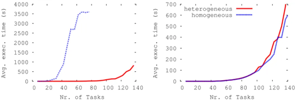
For the test cases obtained using the first algorithm of Section 4.1, the solving times for instances of the same scheduling problem with the same load and the same number of tasks are averaged. The resulting average values are plotted separately for each scheduling problem and load value against the number of tasks. The resulting curve for preemptive, multi-periodic, heterogenous systems with 75% average load, under schedulability analysis, is provided in Fig. 3(left graph, dotted blue curve).
0 500 1000 1500 2000 2500 3000 3500 4000 0 20 40 60 80 100 120 140
Avg. exec. time (s)
Nr. of Tasks 0 100 200 300 400 500 600 700 0 20 40 60 80 100 120 140
Avg. exec. time (s)
Nr. of Tasks heterogeneous
homogeneous
Fig. 3: Single-period, non-preemptive vs. Multi-period, preemptive (left) and Heteroge-nous vs. homogeHeteroge-nous (right)
To give a better feeling of how this graph is built, we plotted in Fig. 4(left) the results of each problem instance. Values with the same abscissa are averaged to obtain the blue line. Fig. 4(right) provides the evolution of timeouts as a function of task number. From 50 tasks on solving has a timeout rate of more than 40%, making it unusable in practice. By comparison, Fig. 3(left graph, solid
0 500 1000 1500 2000 2500 3000 3500 4000 0 10 20 30 40 50 60 70 80 Exec. time (s) Nr. of Tasks 0 20 40 60 80 100 0 10 20 30 40 50 60 70 80 Timeouts (%) Nr. of Tasks
Fig. 4: Results for preemptive, multi-periodic, heterogenous systems, 75% load
same average load (schedulability analysis). Clearly, solving scales much better for the second problem. Intuitively, our experiments show that multi-periodic problems are more complex than single-period ones, and preemptive problems are more complex than non-preemptive ones.
Fig. 3(right graph) provides the results for single-period, non-preemptive task systems with 25% average load in the heterogenous and homogenous case (without symmetry breaking). The graph shows no significant differences, but we shall see later that the use of symmetry breaking should allow a significant reduction of the solving time in the homogenous case if split/merge parallelism is used (so that some homogenous problems are a lot easier to solve).
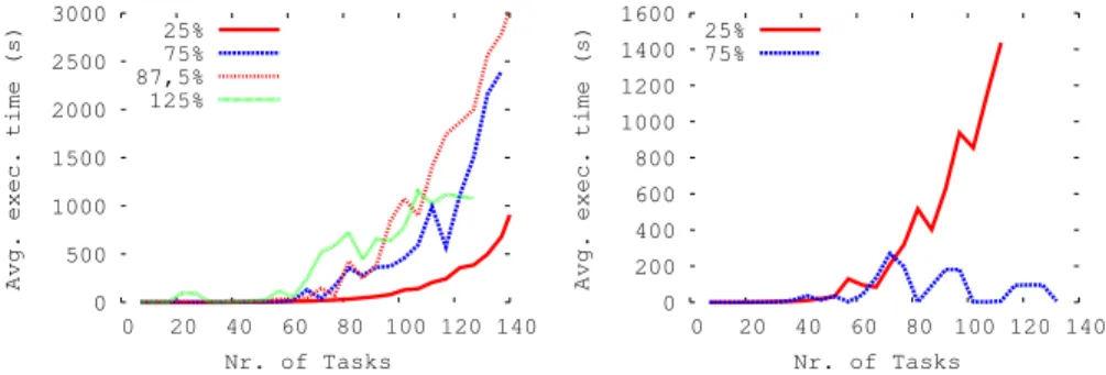
0 500 1000 1500 2000 2500 3000 0 20 40 60 80 100 120 140
Avg. exec. time (s)
Nr. of Tasks 25% 75% 87,5% 125% 0 200 400 600 800 1000 1200 1400 1600 0 20 40 60 80 100 120 140
Avg. exec. time (s)
Nr. of Tasks 25%
75%
Fig. 5: Complexity as a function of system load. Single-period, non-preemptive, het-erogenous (left), Multi-period, non-preemptive, hethet-erogenous (right).
Fig. 5 shows the evolution of the empyric complexity of a problem as a function of the system load. The left graph show that for single-period, non-preemptive, heterogenous schedulability problems, solving scales very well for systems with either very low load (25% on average, solid red line) or very high (over-)load (125% on average, solid green line). In the first case, it is very easy to find solutions. In the second case, non-schedulability is rapidly determined. The remaining two lines correspond to systems with average load, where solving does not scale well. The right graph of the figure considers the multi-period, non-preemptive, heterogenous schedulability problem, where at 75% load solving scales indefinitely (most problems are non-schedulable), whereas at 25% load solving does not scale well.
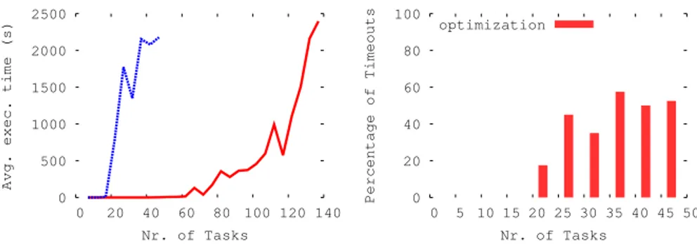
Fig. 6(left) compares the scalability of schedulability analysis (red solid line) with that of period optimization (blue dotted line). The optimization problem is far more complex and does not scale beyond 25 tasks, where the timeout rate is 40% (cf. right graph).
For the test cases obtained using the second algorithm of Section 4.1, we first determined that the solving time for a dependent task problem is always greater or equal that the solving time for the corresponding problem without
0 500 1000 1500 2000 2500 0 20 40 60 80 100 120 140
Avg. exec. time (s)
Nr. of Tasks 0 20 40 60 80 100 0 5 10 15 20 25 30 35 40 45 50 Percentage of Timeouts Nr. of Tasks optimization
Fig. 6: Schedulability analysis vs. optimization for single-period, non-preemptive, het-erogenous at 75% average load
the dependence-related constraints. Furthermore, the global timeout rate for dependent tasks is 55%, whereas for non-dependent tasks is only 13%.
5.2 Signal processing case studies
FFT. The solver was only able to produce optimal schedules for small problems (12 tasks and 16 dependencies), which is consistent with our synthetic example experiments. Note that we were unable to exploit here the symmetry breaking technique, because the FFT task graph does not use split/merge parallelism.
Table 1: Fast Fourier Transform CP resolution time at different levels of the recursion
FFT size (n. of inputs) n. of tasks (messages) opt. time (s) mem. peak (MB)
2 1(0) 0.5 4 4 4(4) 1 4 8 12(16) 2 18 16 32(48) > 1800 271 32 80(128) > 1800 > 8000 64 192(320) > 1800 > 8000
Table 2: CP solver optimisation: time(s), memory(MB) problem performance when raising the breadth of the graph
Symmetry breaking
X (p=1) n.of tasks (messages) None Task CPU Both
0 7 (7) 0.7 2 0.7 2 0.7 2 0.7 2
1 11 (14) 0.9 18 0.7 7 0.7 5 0.6 5
2 15 (21) 5.4 28 1.5 28 2.9 26 1.1 20
Platooning. The experiments show that the solver handles better a very deep task graph than a very large graph. Given the results, a problem with higher depth is expected to be solved within reasonable time as long as the memory of the machine is not exhausted. On contrary, with a problem of large breadth, the solver will not fill the memory of the machine, but will fail to return a solution within reasonable time. Symetry breaking is not trivial in this application graph but can still be achieved if the lexicographic order is the same for Sobel H X and Histo H X.
Table 3: CP solver optimisation problem performance when raising the depth of the graph p (X=0) 1 2 3 4 5 6 7 8 9 10 11 12 13 n.of tasks 7 14 21 28 35 42 49 56 63 70 77 84 91 n.of messages 7 14 22 30 38 46 54 62 70 78 86 94 102 opt time(s) 0.4 0.8 1.2 2 3.2 4.9 7.2 11.3 17.6 21 26 28 > 300 mem peak (MB) 4 10 21 89 199 426 701 1195 1882 2936 4143 5872 > 8000
6
Conclusion
There is a constant mutual challenge between solvers efficiency and problems complexity: new needs from scheduling theory (in temporal correctness) and formal verification theory (functional correctness) raise new interest in resolution techniques, which at some points in history prompt advances in tool power (BDD symbolic representation, SAT/SMT solvers, partial-order and symmetry-based problem reductions,...). One is thus bound to periodically revise judgements on whether the current state-of-affairs in solvers allows to cope with reasonable size specifications, or how far it does.
We tried to provide an empirical answer of that sort (valid as of today), by checking a number of real-time scheduling problems, with typical features repre-sentative of real case-studies. We submitted them to state-of-the art constraint solvers, using optimizing symmetry assumptions, and got answers beyond a sim-ple yes/no, showing that exact computation techniques can indeed be currently attempted on certain problems, provided much care is taken into the solver-aware specification encoding. At the same time, solving complex scheduling problems is likely to require heuristics for some time, especially given the trend of considering larger systems and adding more detail to the specifications.
Recently the Boolean satisfaction modulo theory priniciple was extended to ILP modulo theory [9]. One could wonder at that point how our current contri-bution could fit in a (much more ambitious) idea of a general Constraint modulo theory.
All test cases can be obtained by request to the PC chairs and will be shortly published online, along with the generation scripts, to allow reproduction and extension.
References
1. Bahn, J.H., Yang, J., Bagherzadeh, N.: Parallel fft algorithms on network-on-chips. In: Proceedings ITNG 2008 (April 2008)
2. Baptiste, P., Le Pape, C., Nuijten, W.: Constraint-based scheduling: applying con-straint programming to scheduling problems, vol. 39. Springer Science & Business Media (2001)
3. Bini, E., Buttazzo, G.: Measuring the performance of schedulability tests. Real Time Systems 30, 129–154 (2005)
4. Carle, T., Potop-Butucaru, D.: Predicate-aware, makespan-preserving software pipelining of scheduling tables. TACO 11(1), 12 (2014)
5. Coffman Jr, A.P.E., Graham, R.L.: Optimal scheduling for two-processor systems. Acta informatica 1(3), 200–213 (1972)
6. Craciunas, S., Oliver, R.S.: SMT-based task- and network-level static schedule generation for time-triggered networked systems. In: Proceed-ings RTNS’14. pp. 45:45–45:54. ACM, New York, NY, USA (2014), http://doi.acm.org/10.1145/2659787.2659812
7. Garey, M., Johnson, D.: Complexity results for multiprocessor scheduling under resource constraints. SIAM Journal of Computing 4(4), 397–411 (1975)
8. Gu, Z., He, X., Yuan, M.: Optimization of static task and bus access schedules for time-triggered distributed embedded systems with model-checking. In: Design Au-tomation Conference, 2007. DAC ’07. 44th ACM/IEEE. pp. 294–299 (June 2007) 9. Hang, C., Manolios, P., Papavasileiou, V.: Synthesizing cyber-physical architectural models with real-time constraints. In: Computer Aided Verification. pp. 441–456. Springer (2011)
10. Leyton-Brown, K., Hoos, H.H., Hutter, F., Xu, L.: Understanding the empirical hardness of np-complete problems. Commun. ACM 57(5), 98–107 (May 2014), http://doi.acm.org/10.1145/2594413.2594424
11. Megel, T., Sirdey, R., David, V.: Minimizing task preemptions and migrations in multiprocessor optimal real-time schedules. In: Real-Time Systems Symposium (RTSS), 2010 IEEE 31st. pp. 37–46 (Nov 2010)
12. Nowatzki, T., Sartin-Tarm, M., Carli, L.D., Sankaralingam, K., Es-tan, C., Robatmili, B.: A general constraint-centric scheduling frame-work for spatial architectures. SIGPLAN Not. 48(6), 495–506 (Jun 2013), http://doi.acm.org/10.1145/2499370.2462163, (Proceedings PLDI’13)
13. Tendulkar, P., Poplavko, P., Maler, O.: Symmetry breaking for multi-criteria map-ping and scheduling on multicores. In: Formal Modeling and Analysis of Timed Systems, pp. 228–242. Springer (2013)
14. Topcuoglu, H., Hariri, S., Wu, M.Y.: Performance-effective and low-complexity task scheduling for heterogeneous computing. Parallel and Distributed Systems, IEEE Transactions on 13(3), 260–274 (Mar 2002)