HAL Id: halshs-00118797
https://halshs.archives-ouvertes.fr/halshs-00118797
Submitted on 6 Dec 2006
HAL is a multi-disciplinary open access archive for the deposit and dissemination of sci-entific research documents, whether they are pub-lished or not. The documents may come from teaching and research institutions in France or abroad, or from public or private research centers.
L’archive ouverte pluridisciplinaire HAL, est destinée au dépôt et à la diffusion de documents scientifiques de niveau recherche, publiés ou non, émanant des établissements d’enseignement et de recherche français ou étrangers, des laboratoires publics ou privés.
Innovation and firm growth in ”complex technology”
sectors: a quantile regression approach
Alex Coad, Rekha Rao
To cite this version:
Alex Coad, Rekha Rao. Innovation and firm growth in ”complex technology” sectors: a quantile regression approach. 2006. �halshs-00118797�
Maison des Sciences Économiques, 106-112 boulevard de L'Hôpital, 75647 Paris Cedex 13
http://mse.univ-paris1.fr/Publicat.htm
Centre d’Economie de la Sorbonne
UMR 8174
Innovation and Firm Growth in «Complex Technology» Sectors!: A Quantile Regression Approach
Alex COAD
Rekha RAO
Innovation and Firm Growth in ‘Complex Technology’
Sectors: A Quantile Regression Approach
∗
Alex Coad
? ‡ †Rekha Rao
‡? CES-Matisse, UMR 8174 CNRS et Univ. Paris 1
‡ S.Anna School of Advanced Studies, Pisa, Italy
Cahiers de la MSE
S´
erie rouge
Cahier num´
ero R06050
Abstract
Innovation is commonly seen as the principal engine of economic development. In this paper, we investigate the microfoundations of economic growth by relating innova-tion to sales growth at the firm-level, for incumbent firms in four ‘complex technology’ sectors. The average firm, which experiences only modest growth, may grow for a num-ber of reasons that may or may not be related to ‘innovativeness’. However, given that firms are heterogeneous and that growth rates distributions are typically heavy-tailed, it may be misleading to use regression techniques that focus on the average firm. Using a quantile regression approach, we observe that innovativeness is of crucial importance for a handful of ‘superstar’ fast-growth firms.
INNOVATION ET CROISSANCE DES FIRMES DANS LES SECTEURS DE ‘TECH-NOLOGIES COMPLEXES’ : UNE APPROCHE PAR LA REGRESSION PAR QUAN-TILE
R´esum´e: L’innovation est largement reconnue comme ´etant le moteur principal du d´eveloppement ´economique. Dans ce papier, nous ´etudions les fondements micro de la croissance ´economique en liant l’innovation `a la croissance du chiffre d’affaires au niveau de l’entreprise, pour les firmes ap-partenant `a 4 secteurs de ‘technologies complexes’. L’entreprise moyenne, dont la croissance est faible, croˆıt peut-ˆetre pour des raisons qui n’ont rien `a voir avec l’innovation. N´eanmoins, ´etant donn´e que les firmes sont h´et´erog`enes et que les distributions de taux de croissance sont typique-ment exponentielles, il serait peut-ˆetre erron´e d’appliquer une strat´egie de r´egression centr´ee sur la firme moyenne. Une approche par la r´egression par quantile fait apparaˆıtre que l’innovation est d’une importance primordiale pour un petit nombre de firmes ‘superstars’ ayant un fort taux de croissance.
JEL codes: O31, L25
Keywords: Innovation, Firm Growth, Quantile Regression
Mots cl´es: Innovation, Croissance des firmes, R´egression par quantile
∗Thanks go to Ashish Arora, Giovanni Dosi, Bronwyn Hall, Stephen Machin, Peter Maskell, Stan
Met-calfe, Bernard Paulr´e, Toke Reichstein, and participants at the DRUID Summer conference 2006 for helpful discussions and comments. Each author blames the other for any remaining mistakes.
†Corresponding Author : Alex Coad, CES-Matisse, Maison des Sciences Economiques, 106-112 Bd. de l’Hˆopital, 75647 Paris, France E-mail: [email protected]
1
Introduction
Early contributions on firm growth focused on the empirical validation of Gibrat’s Law, also known as the Law of Proportionate Effect. Taken in its simplest form, this ‘law’ predicts that expected growth rates are independent of firm size. Regressions have found, in general, that growth patterns in modern economies are characterized by a weak negative dependence of growth rates on size (i.e. a slight reversion to the mean), leading us to reject Gibrat’s Law (among a large number of studies see for example Mansfield 1962, Hall 1987, Evans 1987, Hart and Oulton 1996; see also Sutton 1997 for a review). Mean-reversion is typically quite pronounced for small firms, but is much weaker or even nonexistent for larger firms (Mowery (1983), Hart and Oulton (1996), Lotti et al. (2003)). However, the explanatory power of such regressions is often found to be rather low, and the coefficient estimates, though significant, are often quite small. Although strictly speaking we are led to reject Gibrat’s Law, it does appear to be useful as a rough first approximation.
Attention has also been placed on the influence of other factors on firm growth, using a variety of different databases. One classic research topic has been to investigate the influence of age on firm growth. Indeed, it has even been suggested that the correct causality runs from age to size to growth, such that size has no effect on the expected growth rates if age is taken into account (Fizaine 1968, Evans 1987). In any case, age is observed to have a negative influence on firm growth. Legal status seems to have an influence, with public firms and firms with limited liability having significantly higher growth rates in comparison with other companies (Harhoff et al. 1998). Proprietary structure also appears to affect growth, when this latter is taken at the plant-level. Evidence suggests that the expected growth rate of a plant declines with size for plants owned by single-plant firms but increases with size for plants owned by multiplant firms (Dunne et al. 1989). Looking at data on industry leaders, Geroski and Toker (1996) identify other variables that are observed to influence growth. Advertising expenditure, the demand growth of an industry, and also the industry concentration are observed to have a positive influence on firm growth rates.
However, even though such explorations into the determinants of firm growth rates may obtain coefficient estimates that are statistically significant, the explanatory power is
remark-ably weak (Geroski 2000). As Marsili (2001) points out, the R2 coefficient in such studies is
generally lower than 30%. “In short, the empirical evidence suggests that although there are systematic factors at the firm and industry levels that affect the process of firm growth, growth is mainly affected by purely stochastic shocks. . . ” (Marsili 2001:18). “The most elementary ‘fact’ about corporate growth thrown up by econometric work on both large and small firms is that firm size follows a random walk” (Geroski 2000:169). It seems that there is little more that we can say about firm growth rates apart from that they are largely unpredictable, stochastic, and idiosyncratic. However, as Geroski (2000) concludes, these characteristics of growth rates may be due to the unpredictable and stochastic nature of innovation success; i.e. that looking at firm-level innovations could be the key to understanding firm-level growth. We believe that this idea deserves further empirical investigation.
One of the difficulties in observing the effect of innovation on growth is that it may take a firm a long time to convert increases in economically valuable knowledge (i.e. innovation) into economic performance. Even after an important discovery has been made, a firm will typically have to invest heavily in product development. In addition, converting a product idea into a set of successful manufacturing procedures and routines may also prove costly and difficult. Furthermore, even after an important discovery has been patented, a firm in an uncertain market environment may prefer to treat the patent as a ‘real option’ and delay associated
investment and development costs (Bloom and Van Reenen, 2002). There may therefore be considerable lags between the time of discovery of a valuable innovation and its conversion into commercial success. Another feature of the innovation process is that there is uncertainty at every stage, and that the overall outcome requires success at each step of the process. In a pioneering empirical study, Mansfield et al. (1977) identify three different stages of innovation that correspond to three different conditional probabilities of success: the probability that a project’s technical goals will be met (x); the probability that, given technical success, the resulting product or process will be commercialized (y); and finally the probability that, given commercialization, the project yields a satisfactory return on investment (z). The overall success of the innovative activities will be the product of these three conditional probabilities (x × y × z). If a firm fails at any of these stages, it will have incurred costs without reaping benefits. We therefore expect that firms differ greatly both in terms of the returns to R&D (measured here in terms of post-innovation sales growth) and also in terms of the time required to convert an innovation into commercial success. However, it is anticipated that innovations will indeed pay off on average and in the long term, otherwise commercial businesses would obviously have no incentive to perform R&D in the first place.
One strand of the empirical literature has focused on the influence of firm-level innovation on employment growth, exploring the popular concern that technological advance is labour-saving and thus necessarily leads to technological unemployment (see, among others, Van Reenen 1997, Greenhalgh et al. 2001, and Evangelista and Savona 2003). A successful in-novator may grow by changing the composition of its productive resources, to the profit of machines and at the expense of employment. Even if the innovating firm grows significantly, a reallocation of production between capital and labour makes the effect of innovation on employment growth a priori unclear. Indeed, it is observed that even “[e]mpirical work on the effect of innovations on employment growth yields very mixed results” (Niefert 2005:9).
An investigation of innovation on sales growth, however, should not be so ambiguous. It is reasonable to expect that successful innovators will grow more than other firms, although the magnitude of the relationship between innovation and growth and the relevant number of time lags are empirical questions. Our gleaning of this literature yields nonetheless a sparse and rather motley harvest. (This may be due to difficulties in linking firm-level innovation data to other firm characteristics.) Mansfield (1962) considers the steel and petroleum sectors over a 40-year period, and finds that successful innovators grew quicker, especially if they were initially small. Moreover, he asserts that the higher growth rate cannot be attributed to their pre-innovation behavior. Another early study by Scherer (1965) looks at 365 of the largest US corporations and observes that inventions (measured by patents) have a positive effect on company profits via sales growth. Of particular interest to this study is his observation that innovations typically do not increase profit margins but instead increase corporate profits via increased sales at constant profit margins. This suggests that sales growth is a particularly meaningful indicator of post-innovation performance. Mowery (1983) focuses on the dynamics of US manufacturing over the period 1921-1946 and observes that R&D employment only has a significantly positive impact on firm growth (in terms of assets) for the period 1933-46. Furthermore, using two different samples, he observes that R&D has a similar effect on growth for both large and small firms. Geroski and Machin (1992) look at 539 large quoted UK firms over the period 1972-83, of which 98 produced an innovation during the period considered. They observe that innovating firms (i.e. firms that produced at least one ‘major’ innovation) are both more profitable and grow faster than non-innovators. The influence of specific innovations on sales growth are nonetheless short-lived (p. 81) - “the full effects of innovation on corporate growth are realized very soon after an innovation is introduced,
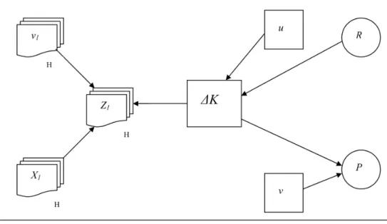
Figure 1: The Knowledge ‘Production Function’: A Simplified Path Analysis Diagram (from Griliches 1990:1671)
generating a short, sharp one-off increase in sales turnover.” In addition, and contrary to Scherer’s findings, they observe that innovativeness has a more noticeable influence on profit margins than on sales growth. Geroski and Toker (1996) look at 209 leading UK firms and observe that innovation has a significant positive effect on sales growth, when included in an OLS regression model amongst many other explanatory variables. Roper (1997) uses survey data on 2721 small businesses in the U.K., Ireland and Germany to show that innovative products introduced by firms made a positive contribution to sales growth. Freel (2000) considers 228 small UK manufacturing businesses and, interestingly enough, observes that although it is not necessarily true that ‘innovators are more likely to grow’, nevertheless ‘innovators are likely to grow more’ (i.e. they are more likely to experience particularly rapid growth). Finally, Bottazzi et al. (2001) study the dynamics of the worldwide pharmaceutical sector and do not find any significant contribution of a firm’s ‘technological ID’ or innovative
position1 to sales growth.
A critical examination of these studies reveals that the proxies that they use to quantify ‘innovativeness’ are rather noisy. Figure 1 shows that the variable of interest (i.e. ∆K - addi-tions to economically valuable knowledge) is measured with noise if one takes either innovative input (such as R&D expenditure or R&D employment) or innovative output (such as patent statistics). In order to remove this noise, one needs to collect information on both innovative input and output, and to extract the common variance whilst discarding the idiosyncratic vari-ance of each individual proxy that includes noise, measurement error, and specific variation. In this study, we believe we have obtained useful data on a firm’s innovativeness by considering
1They measure a firm’s innovativeness by either the discovery of NCE’s (new chemical entities) or by the
both innovative input and innovative output simultaneously in a synthetic variable.2 Another criticism is that previous studies have lumped together firms from all manufacturing sectors - even though innovation regimes vary dramatically across industries. In this study, we focus on specific 2-digit sectors that have been hand-picked according to their intensive patenting and R&D activity. However, even within 2-digit sectors, there is significant heterogeneity between firms, and using standard regression techniques to make inferences about the average firm may mask important phenomena. Using quantile regression techniques, we investigate the relationship between innovativeness and growth at a range of points of the conditional growth rate distribution. We observe that, whilst for the average firm innovativeness may not be so important for sales growth, innovativeness is of crucial importance for the ‘superstar’ high-growth firms.
“Linking more explicitly the evidence on the patterns of innovation with what is known about firms growth and other aspects of corporate performance - both at the empirical and at the theoretical level - is a hard but urgent challenge for future research” (Cefis and Ors-enigo, 2001:1157). We are now in a position to rise to this challenge. In section 2 we discuss the methodology, focusing in particular on the shortcomings of using either patent counts or R&D figures individually as proxies for innovativeness. We describe how we use Princi-pal Component Analysis to extract a synthetic ‘innovativeness’ index from patent and R&D data. Section 3 describes how we matched the Compustat database to the NBER innova-tion database. In secinnova-tion 4 we proceed to a regression analysis. In secinnova-tion 5 we provide a brief introduction to quantile regression techniques and apply them to our context. Section 6 concludes.
2
Methodology - How can we measure innovativeness?
Activities related to innovation within a company can include research and development; acquisition of machinery, equipment and other external technology; industrial design; and training and marketing linked to technological advances. These are not necessarily identified as such in company accounts, so quantification of related costs is one of the main difficulties encountered during the innovation studies. Each of the above mentioned activities has some effect on the growth of the firm, but the singular and cumulative effect of each of these activities is hard to quantify. Data on innovation per se has thus been hard to find (Van Reenen, 1997). Also, some sectors innovative extensively, some don’t innovative in a tractable manner, and the same is the case with organizational innovations, which are hard to quantify in terms of impact on the overall growth of the firms. However, we believe that no firm can survive without at least some degree of innovation.
We use two indicators for innovation in a firm: first, the patents applied for by a firm and second, the amount of R&D undertaken. Cohen et al. (2000) suggest that no industry relies exclusively on patents, yet the authors go on to suggest that the patents may add sufficient value at the margin when used with other appropriation mechanisms. Although patent data has drawbacks, patent statistics provide unique information for the analysis of the process of technical change (Griliches, 1990). We can use patent data to access the patterns of innova-tion activity across fields (or sectors) and nainnova-tions. The number of patents can be used as an
2Following Griliches (1990), we consider here that patent counts can be used as a measure of innovative
output, although this is not entirely uncontroversial. Patents have a highly skew value distribution and many
patents are practically worthless. As a result, patent numbers have limitations as a measure of innovative output - some authors would even prefer to consider raw patent counts to be indicators of innovative input.
indicator of inventive as well as innovative activity, but it has its limitations. One of the major disadvantage of patents as an indicator is that not all inventions and innovations are patented (or indeed ‘patentable’). Some companies - including a number of smaller firms - tend to find the process of patenting expensive or too slow and implement alternative measures such as secrecy or copyright to protect their innovations (Archibugi 1992; Arundel and Kabla 1998). Another bias in the study using patenting can arise from the fact that not all patented inven-tions become innovainven-tions. The actual economic value of patents is highly skewed and varying, and most of the value is concentrated in a very small percentage of the total (OECD, 1994). Furthermore, another caveat of using patent data is that we may underestimate innovation occuring in large firms, because these typically have a lower propensity to patent (Dosi 1988). The reason we use patent data in our study is that, despite the problems mentioned above, patents would reflect the continuous developments within technology (Engelsman and van Raan, 1990). We complement the patent data with R&D data. R&D can be considered as an input into the production of inventions, and patents as intermediates into the production of innovations. R&D data may lead us to systematically underestimate the amount of innovation in smaller firms, however, because these often innovate on a more informal basis outside of the R&D lab (Dosi 1988). For some of the analysis we consider the R&D stock and also the patent stock, since the past investments in R&D as well as the past applications of patents have an impact not only on the future values of R&D and patents, but also on firm growth. Hall (2004) suggests that the past history of R&D spending is a good indicator of the firms technological position.
Taken individually, each of these indicators for firm-level innovativeness has its drawbacks. Each indicator on its own provides useful information on a firm’s innovativeness, but also idiosyncratic variance that may, at best, be unrelated to a firm’s innovativeness. One particular feature pointed out by Griliches (1990) is that, although patent data and R&D data are often chosen to individually represent the same phenomenon, there exists a major statistical discrepancy in that there is typically a great randomness in patent series, whereas R&D/sales ratios are much more smoothed. Principal Component Analysis (PCA) is appropriate here as it allows us here to summarize the information provided by several indicators of innovativeness into a composite index, by extracting the common variance from correlated variables whilst separating it from the specific and error variance associated with each individual variable (Hair
et al. 1998). We are not the only ones to apply PCA to studies into firm-level innovation
however - this technique has also been used by Lanjouw and Schankerman (2004) to develop a composite index of ‘patent quality’ using multiple characteristics of patents (such as the number of citations, patent family size and patent claims).
We only consider certain specific sectors, and not the whole of manufacturing. This way we are not affected by aggregation effects; we are grouping together firms that can plausibly be compared to each other. We are particularly interested in looking at the growth of firms clas-sified under ‘complex’ technology classes. We base our classification of firms on the typology
put forward by Hall (2004) and Cohen et al. (2000). The authors define ‘complex product’3
industries as those industries where each product relies on many patents held by a number of other firms and the ‘discrete product’ industries as those industries where each product relies on only a few patents and where the importance of patents for appropriability has
tradition-ally been higher.4 We chose four sectors that can be classified under the ‘complex products’
3During our discussion, we will use the terms ‘products’ and ‘technology’ interchangeably to indicate
gen-erally the same idea.
4It would have been interesting to include ‘discrete technology’ sectors in our study, but unfortunately we
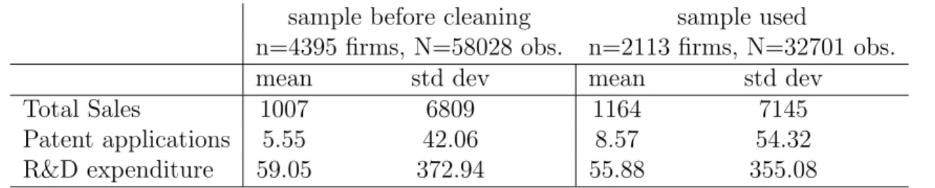
Table 1: Summary statistics before and after data-cleaning
sample before cleaning sample used
n=4395 firms, N=58028 obs. n=2113 firms, N=32701 obs.
mean std dev mean std dev
Total Sales 1007 6809 1164 7145
Patent applications 5.55 42.06 8.57 54.32
R&D expenditure 59.05 372.94 55.88 355.08
Note: for R&D, n=4009, N =44641 before cleaning; n=2113, N =32326 after cleaning.
class. The two digit SIC codes that match the ‘complex technology’ sectors are 35, 36, 37,
and 38.5 By choosing these sectors that are characterised by high patenting and high R&D
expenditure, we hope that we will be able to get the best possible quantitative observations for firm-level innovation.
3
Database
We use an original database created from the NBER patent database and the Compustat file database for our study, and this section is devoted to describing the creation of the sample which we will use in our analysis.
The innovation data has been obtained from the NBER Database (Hall et al. 2001b). The NBER database comprises detailed information on almost 3,416,957 U.S. utility patents in the USPTO’s TAF database granted during the period 1963 to December 2002 and all citations made to these patents between 1975 and 2002. The firms patenting history is analysed over the whole period represented by the NBER patent database. The initial sample of firms was
obtained from the Compustat6 database for the aforementioned sectors comprising ’complex’
product sectors. These firms were then matched with the firm data files from the NBER
patent database and we found all the firms7 that have patents. The final sample thus contains
5The ‘complex technology’ sectors that we consider are SIC 35 (industrial and commercial machinery and
computer equipment), SIC 36 (electronic and other electrical equipment and components, except computer equipment), SIC 37 (transportation equipment) and SIC 38 (measuring, analyzing and controlling instruments; photographic, medical and optical goods; watches and clocks).
6Compustat has the largest set of fundamental and market data representing 90% of the worlds market
capitalization. Use of this database could indicate that we have oversampled the Fortune 500 firms. Being included in the Compustat database means that the number of shareholders in the firm was large enough for the firm to command sufficient investor interest to be followed by Standard and Poor’s Compustat, which basically means that the firm is required to file 10-Ks to the Securities and Exchange Commission on a regular basis. It does not necessarily mean that the firm has gone through an IPO. Most of them are listed on NASDAQ or the NYSE.
7The patent ownership information (obtained from the above mentioned sources) reflects ownership at the
time of patent grant and does not include subsequent changes in ownership. Also attempts have been made to combine data based on subsidiary relationships. However, where possible, spelling variations and variations based on name changes have been merged into a single name. While every effort is made to accurately identify all organizational entities and report data by a single organizational name, achievement of a totally clean record is not expected, particularly in view of the many variations which may occur in corporate identifications. Also, the NBER database does not cumulatively assign the patents obtained by the subsudiaries to the parents, and we have taken this limitation into account and have subsequently tried to cumulate the patents obtained by the subsidiaries towards the patent count of the parent. Thus we have attempted to create an original database
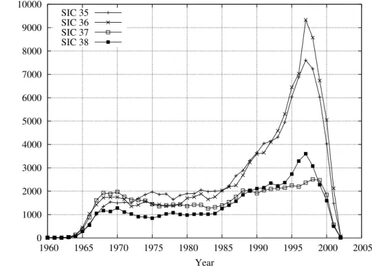
0 1000 2000 3000 4000 5000 6000 7000 8000 9000 10000 1960 1965 1970 1975 1980 1985 1990 1995 2000 2005 No. Patents Year SIC 35 SIC 36 SIC 37 SIC 38
Figure 2: Number of patents per year. SIC 35: Machinery & Computer Equipment, SIC 36: Electric/Electronic Equipment, SIC 37: Transportation Equipment, SIC 38: Measuring Instruments.
both patenters and non-patenters.
The NBER database has patent data for over 60 years and the Compustat database has firms’ financial data for over 50 years, giving us a rather rich information set. As Van Reenen (1997) mentions, the development of longitudinal databases of technologies and firms is a major task for those seriously concerned with the dynamic effect of innovation on firm growth. Hence, having developed this longitudinal dataset, we feel that we will be able to thoroughly investigate whether innovation drives sales growth at the firm-level.
Table 1 shows some descriptive statistics of the sample before and after cleaning. Initially using the Compustat database, we obtain a total of 4395 firms which belong to the SICs 35-38 and this sample consists of both innovating and non-innovating firms. These firms were then matched to the NBER database. After this initial match, we further matched the year-wise firm data to the year-wise patents applied by the respective firms (in the case of innovating firms) and finally, we excluded firms that had less than 7 consecutive years of good data. Thus, we have an unbalanced panel of 2113 firms belonging to 4 different sectors. Since we intend to take into account sectoral effects of innovation, we will proceed on a sector by sector basis, to have (ideally) 4 comparable results for 4 different sectors.
Figure 2 shows the number of patents per year in our final database. For two of the sectors (i.e. 35 and 36), there appears to be a strong structural break at the beginning of the 1980s which may well be due to changes in patent regulations (see Hall (2004) for a discussion). Table 2 presents the firm-wise distribution of patents, which is noticeably right-skewed. We find that 47% of the firms in our sample have no patents. Thus the intersection of the two datasets gave us 1129 patenting firms who had taken out at least one patent between 1963
Table 2: The Distribution of Firms by Total Patents, 1963-1999
0 or more 1 or more 10 or more 25 or more 100 or more 250 or more 1000 or more
Firms 2113 1122 733 511 222 128 56
Table 3: Contemporaneous correlations
between Patents and R&D expenditure
SIC 35 SIC 36 SIC 37 SIC 38
Corr. 0.5392 0.3411 0.4996 0.6720
p-value 0.0000 0.0000 0.0000 0.0000
Obs. 10017 10222 3175 8912
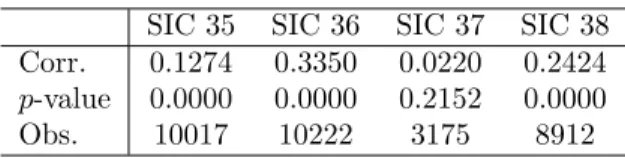
Table 4: Contemporaneous correlations be-tween ‘patent intensity’ (patents/sales) and ‘R&D intensity’ (R&D/sales)
SIC 35 SIC 36 SIC 37 SIC 38
Corr. 0.1274 0.3350 0.0220 0.2424
p-value 0.0000 0.0000 0.2152 0.0000
Obs. 10017 10222 3175 8912
and 1999, and 991 firms that had no patents during this period. The total number of patents taken out by this group over the entire period was 332 888, where the entire period for the NBER database represented years 1963 to 2002, and we have used 269 102 of these patents in our analysis i.e. representing about 81% of the total patents ever taken out at the US Patent Office by the firms in our sample. Though the NBER database provides the data on patents applied for from 1963 till 2002, it contains information only on the granted patents and hence we might see some bias towards the firms that have applied in the end period covered by the database due the lags faced between application and the grant of the patents. Hence to avoid this truncation bias (on the right) we consider the patents only till 1999 so as to account for
the average 3-year gap between application and grant of the patent.8 Concerning R&D, 2100
of the 2113 firms report positive R&D expenditure, and 2078 of these report R&D for more than seven years.
Table 3 shows that patent numbers are well correlated with total R&D expenditure, albeit without controlling for firm size. To take this into account, Table 4 reports the correlations between firm-level patent intensity and R&D intensity. For sectors 35, 36 and 38 we observe positive and highly significant correlations, which nonetheless take values of 0.335 or lower. These correlations coefficients would thus appear to be consistent with the idea that, even within industries, patent and R&D statistics do contain large amounts of idiosyncratic vari-ance and that either of these variables taken individually would be a rather noisy proxy for ‘innovativeness’.
4
Regression Analysis
To investigate the long-term influence of innovation on growth, we turn to regression estimation of equations (1) and (2), on a sector by sector basis.
GROW T Hi,t = α1GROW T Hi,t−1+ α2SIZEi,t−1+ K
X
k=1
βkP ATi,t−k+ yt+ νi+ ²i,t (1)
8This average gap has been referred to by many authors, among others Bloom and Van Reenen (2002) who
mention a lag of two years between application and grant, and Hall et al. (2001a) who state that 95% of the patents that are eventually granted are granted within 3 years of application.
T able 5: In vestigating the relev ance of lagged paten t in tensit y on gro wth -estimation of Equation (1). a Dep.V ar. SIC 35 SIC 36 SIC 37 SIC 38 Gro wth (t -1: t) OLS FE GMM OLS FE GMM OLS FE GMM OLS FE GMM P at/Sales (t − 1) 0.0440 0.0354 0.0243 0.0207 0.0267 0.0184 -0.0478 -0.0219 -0.0513 0.0017 0.0021 0.0018 (t -stat) 1.24 0.72 1.89 1.31 2.05 1.71 -1.85 -0.84 -2.05 4.62 2.34 11.35 (t − 2) 0.0140 0.0171 0.0107 0.0029 0.0010 -0.0012 0.0609 0.0674 0.0622 0.0010 0.0013 0.0011 (t -stat) 0.70 0.59 1.84 0.18 0.06 -0.12 1.67 1.97 3.60 10.81 1.42 9.08 (t − 3) -0.0144 0.0013 -0.0124 0.0016 0.0017 -0.0002 0.1122 0.1059 0.1193 0.0001 4.25 E-05 -1.05 E-05 (t -stat) -0.60 0.09 -2.06 6.93 3.35 -0.07 3.67 4.04 13.70 0.37 0.14 -0.06 Obs. N =7368 N =7368 N =7368 N =7564 N =7564 N =7564 N =2510 N =2510 N =2510 N =6571 N =6571 N =6571 n =668 n =668 n =676 n =676 n =185 n =185 n =579 n =579 R 2 within 0.0436 0.0419 0.0876 0.0441 R 2 b et w een 0.0013 0.0088 0.0464 0.1710 R 2 ov erall 0.0491 0.0198 0.0477 0.0194 0.1046 0.0572 0.0206 0.0097 F -stat -10.52 214.16 12.94 9.19 1.46 E+12 6.53 6.43 1.86 E+07 -9.81 E+09 422492 Hansen J (p -v alue) b 0.984 0.985 1.000 0.776 AR(1) p-v alue 0.000 0.000 0.000 0.000 AR(2) p-v alue 0.445 0.805 0.750 0.252 aCo efficien ts significan t at the 5% lev el app ear in b old. P at/Sales = paten ts( t)/sales( t − 1), R&D/Sales = R&D( t)/sales( t − 1); inno vation pro xies( t) are deflated b y sales at time t − 1 to av oid problems related to the ’regression fallacy’. SIC 35: Mac hinery & Computer Equipmen t, SIC 36: Electric/Electronic Equipmen t, SIC 37: T ransp ortation Equipmen t, SIC 38: Measuring Instrumen ts. bT ests for ov er-iden tifying restrictions usually giv e Sargan statistics. Ho w ev er, w e prefer the Hansen J statistic here, since the Sargan statistic is not robust to heterosk edasticit y or auto correlation (Ro o dman 2005). This Hansen J statistic is the (robust) minimized value of the tw o-step GMM criterion function, whereas the Sargan statistic is the minimized value of the one-step GMM criterion function (Ro o dman 2005).
T able 6: In vestigating the relev ance of lagged R&D in tensit y on gro wth -estimation of Equation (2). a Dep.V ar. SIC 35 SIC 36 SIC 37 SIC 38 Gro wth (t -1: t) OLS FE GMM OLS FE GMM OLS FE GMM OLS FE GMM R&D/Sales (t− 1) 0.0285 0.0526 0.0189 0.0085 0.0149 0.0055 0.2363 0.2735 0.2132 0.0003 0.0008 0.0004 (t -stat) 0.70 0.78 0.58 1.32 1.99 0.87 1.36 1.56 2.06 1.42 3.37 1.77 (t − 2) -0.0049 0.0023 -0.0051 -0.0022 -0.0045 -0.0045 -0.2132 -0.2393 -0.2318 0.0006 0.0007 0.0006 (t -stat) -0.27 0.07 -0.48 -0.36 -0.78 -1.55 -1.27 -1.08 -2.84 3.81 4.34 3.89 (t − 3) 0.0007 0.0003 0.0006 0.0030 0.0013 0.0045 0.3127 0.3430 0.3577 0.0002 0.0002 0.0002 (t -stat) 1.05 0.22 1.53 1.36 0.44 1.79 2.21 2.84 5.62 0.99 1.71 1.10 Obs. N =7298 N =7298 N =7298 N =7478 N =7478 N =7478 N =2418 N =2418 N =2418 N =6549 N =6549 N =6549 n =668 n =668 n =676 n =676 n =185 n =185 n =579 n =579 R 2 within 0.0452 0.0417 0.1011 0.0483 R 2 b et w een 0.0008 0.0123 0.0589 0.3436 R 2 ov erall 0.0496 0.0196 0.0475 0.0187 0.1193 0.0716 0.0202 0.0089 F -stat -10.58 127.46 8.45 8.56 1794.19 5.53 5.86 1.27 E+08 -1.45 E+09 75.61 Hansen J (p -v alue) 0.884 0.996 1.000 0.471 AR(1) p-v alue 0.000 0.000 0.000 0.000 AR(2) p-v alue 0.449 0.749 0.757 0.314 aCo efficien ts significan t at the 5% lev el app ear in b old. P at/Sales = paten ts( t)/sales( t − 1), R&D/Sales = R&D( t)/sales( t − 1); inno vation pro xies( t) are deflated b y sales at time t − 1 to av oid problems related to the ’regression fallacy’. SIC 35: Mac hinery & Computer Equipmen t, SIC 36: Electric/Electronic Equipmen t, SIC 37: T ransp ortation Equipmen t, SIC 38: Measuring Instrumen ts.
GROW T Hi,t = α1GROW T Hi,t−1+ α2SIZEi,t−1+ K
X
k=1
βkR&Di,t−k+ yt+ νi+ ²i,t (2)
Sales growth for firm i in year t is taken as the dependent variable, and either ‘patent intensity’ (P AT ) or ‘R&D intensity’ (R&D) features as the independent variable. We control for growth rate autocorrelation by including lagged growth, and also control for size
depen-dence by including lagged sales. The yt are yearly dummy variables, and νi captures the
time-invariant firm-specific fixed effects between firms. We estimate equations (1) and (2) using pooled OLS (in which case the firm-specific fixed effects are not included) and fixed-effects regressions (the relevant test statistics, not shown here, indicate that we should prefer fixed-effects panel data estimation to random effects estimation). The usual OLS assumptions are likely not to be completely satisfied in this dataset, however, and so the reader should not attach too much importance to the OLS estimates. We also report results obtained using the ‘system GMM’ dynamic panel-data estimator (Arellano and Bover (1995), Blundell and Bond (1998)).
Regression results are presented in tables 5 and 6. A first remark is that each sector appears to display slightly different dynamics. For sector 35 (Machinery and Computer Equipment), we are largely unable to discern any significant effect of innovativeness on sales growth. It would appear that patent intensity would have a positive effect on growth one year after, but this positive influence may actually become negative when patent intensity is lagged three years. For sector 36 (Electric/Electronic Equipment), a firm’s innovativeness is associated with superior growth one period later, although the longer-term influence is harder to unravel. Sector 37 (Transportation Equipment) presents some unique results in that the largest influ-ence between innovativeness and growth is visible when three lags are taken. Finally, for sector 38, innovativeness appears to have its greatest effect on growth when one lag is considered, although a somewhat smaller effect can be detected in the second lag.
A comparison of tables 5 and 6 reveals that the two innovativeness variables - patent intensity and R&D intensity - do give results that are sometimes qualitatively different (e.g. the 3rd lag of SIC 36 or the first two lags of SIC 37). Indeed, as discussed in section 2, these two variables are quite different not only in terms of statistical properties (patent statistics are much more skewed and less persistent than R&D statistics) but also in terms of economic significance.
The overall R2 for the regressions is relatively small in all cases: it is highest in sector 37
(up to 12%) but less than 5% for the remaining sectors. It is clear that, by looking at a firm’s ‘innovativeness’, we have not discovered the ‘answer’ or the ‘key’ to understanding variation in firm growth. Innovation is uncertain and generally lacks persistence; similarly, firm growth is highly idiosyncratic and lacks persistence - in the face of this circumstantial evidence, however, we should resist the temptation to overplay the relationship between innovativeness and firm growth.
There is something of a convention in the innovation literature to amortize R&D expen-diture and patents at a rate of 15% (see among others Griliches (1990) and Lanjouw and Schankerman (2004)), and the implications of this particular figure are that a firm’s com-parative advantage in terms of innovativeness will not tend to last more than a few years. Applying this amortizement rate to patents, for example, suggests that one patent today is worth ceteris paribus almost twice as much as a patent four years ago, and more than three times as much as a patent seven years ago. Furthermore, an implication of this constant
Table 7: Extracting the ‘innovativeness’ index used for the quantile regressions - Principal Component Analysis results (first component only, unrotated)
SIC 35 SIC 36 SIC 37 SIC 38
R&D / Sales 0.4321 0.3889 0.4579 0.4126
Patents / Sales 0.3946 0.3340 0.3385 0.4069
R&D stock / Sales (δ = 15%) 0.4005 0.4364 0.4579 0.4078
Patent stock / Sales (δ = 15%) 0.4100 0.4264 0.3562 0.4069
R&D stock / Sales (δ = 30%) 0.4001 0.4328 0.4596 0.4085
Patent stock / Sales (δ = 30%) 0.4112 0.4214 0.3578 0.4069
Propn Variance explained 0.6509 0.7820 0.5135 0.5522
No. Obs. 8611 8796 2773 7698
depreciation rule is that firm-level innovativeness should have a monotonically decreasing in-fluence on firm performance as time goes by. The results presented in tables 5 and 6 are not entirely consistent with this 15% depreciation approach. First, there does not appear to be a monotonically decreasing influence of innovativeness on growth - in sector 37, for example, the largest effect is detectable in the third lag, and for the first two lags the sign of the coefficient changes. Second, the coefficient estimates in sectors 35, 36 and 38 would appear to decay at a faster depreciation rate than 15%. This is consistent with recent remarks that the standard 15% level may be too low (Hall and Oriani, 2006). In any case, the evidence presented here suggests that firm-level R&D and patent stocks display different depreciation dynamics across different sectors.
5
Quantile Regressions
In this section we begin by explaining why we believe quantile regression techniques to be a useful tool to this study. First we describe the intuition of quantile regression analysis, and then we present the quantile regression model in a few introductory equations. In section 5.2 we present the results.
5.1
Methodology
Standard least squares regression techniques provide summary point estimates that calculate the average effect of the independent variables on the average firm. However, this focus on the average firm may hide important features of the underlying relationship. As Mosteller and Tukey explain in an oft-cited passage: “What the regression curve does is give a grand summary for the averages of the distributions corresponding to the set of x’s. We could go further and compute several regression curves corresponding to the various percentage points of the distributions and thus get a more complete picture of the set. Ordinarily this is not done, and so regression often gives a rather incomplete picture. Just as the mean gives an incomplete picture of a single distribution, so the regression curve gives a correspondingly incomplete picture for a set of distributions” (Mosteller and Tukey, 1977:266). Quantile re-gression techniques can therefore help us obtain a more complete picture of the underlying relationship between innovation and firm growth.
In our case, estimation of linear models by quantile regression may be preferable to the usual regression methods for a number of reasons. First of all, we know that the standard least-squares assumption of normally distributed errors does not hold for our database be-cause growth rates follow a heavy-tailed distribution (see Stanley et al. (1996) for the growth rates distribution of Compustat firms). Whilst the optimal properties of standard regression estimators are not robust to modest departures from normality, quantile regression results are characteristically robust to outliers and heavy-tailed distributions. In fact, the quantile
regression solution ˆβθ is invariant to outliers that tend to ± ∞ (Buchinsky, 1994). Another
advantage is that, while conventional regressions focus on the mean, quantile regressions are able to describe the entire conditional distribution of the dependent variable. In the context of this studies, high growth firms are of interest in their own right, we don’t want to dismiss them as outliers, but on the contrary we believe it would be worthwhile to study them in detail. This can be done by calculating coefficient estimates at various quantiles of the conditional distribution. Finally, a quantile regression approach avoids the restrictive assumption that the error terms are identically distributed at all points of the conditional distribution, since the variance-covariance matrix is estimated by bootstrapping techniques. Relaxing this assump-tion allows us to acknowledge firm heterogeneity and consider the possibility that estimated slope parameters vary at different quantiles of the conditional growth rate distribution.
The quantile regression model, first introduced by Koenker and Bassett (1978), can be written as:
yit= x0itβθ+ uθit with Quantθ(yit|xit) = x0itβθ (3)
where yit is the growth rate, x is a vector of regressors, β is the vector of parameters to be
estimated, and u is a vector of residuals. Q(yit|xit) denotes the θth conditional quantile of yit
given xit. The θth regression quantile, 0 < θ < 1, solves the following problem:
min β 1 n ½ X i,t:yit≥x0itβ θ|yit− x0itβ| + X i,t:yit<x0itβ (1 − θ)|yit− x0itβ| ¾ = min β 1 n n X i=1 ρθuθit (4)
where ρθ(.), which is known as the ‘check function’, is defined as:
ρθ(uθit) =
½
θuθit if uθit ≥ 0
(θ − 1)uθit if uθit < 0
¾
(5) Equation (4) is then solved by linear programming methods. As one increases θ con-tinuously from 0 to 1, one traces the entire conditional distribution of y, conditional on x (Buchinsky, 1998). More on quantile regression techniques can be found in the surveys by Buchinsky (1998) and Koenker and Hallock (2001); see also the special issue of Empirical
Economics (Vol. 26 (3), 2001).
5.2
Results
We now seek to estimate the following linear regression model:
GROW T Hi,t = α1GROW T Hi,t−1+ α2SIZEi,t−1+ α3IN Ni,t−k+ yt+ ²i,t (6)
which is similar to the previous models. This time, we create a composite ‘innovativeness’ variable, INN , using Principal Components Analysis (see Table 7). This synthetic ‘innova-tiveness’ index is created by extracting the common variance from a series of related variables:
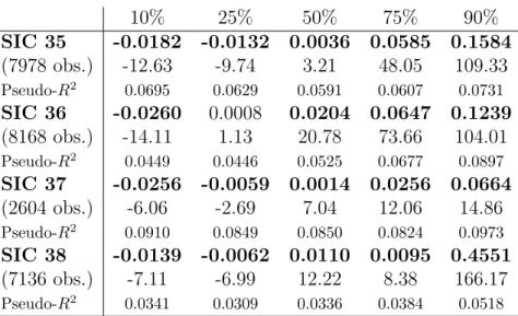
Table 8: Quantile regression estimation of equation (6): the coefficient and t-statistic on ‘in-novativeness’ reported for the 10%, 25%, 50%, 75% and 90% quantiles. Coefficients significant at the 5% level appear in bold.
10% 25% 50% 75% 90% SIC 35 -0.0182 -0.0132 0.0036 0.0585 0.1584 (7978 obs.) -12.63 -9.74 3.21 48.05 109.33 Pseudo-R2 0.0695 0.0629 0.0591 0.0607 0.0731 SIC 36 -0.0260 0.0008 0.0204 0.0647 0.1239 (8168 obs.) -14.11 1.13 20.78 73.66 104.01 Pseudo-R2 0.0449 0.0446 0.0525 0.0677 0.0897 SIC 37 -0.0256 -0.0059 0.0014 0.0256 0.0664 (2604 obs.) -6.06 -2.69 7.04 12.06 14.86 Pseudo-R2 0.0910 0.0849 0.0850 0.0824 0.0973 SIC 38 -0.0139 -0.0062 0.0110 0.0095 0.4551 (7136 obs.) -7.11 -6.99 12.22 8.38 166.17 Pseudo-R2 0.0341 0.0309 0.0336 0.0384 0.0518
both patent intensity and R&D intensity at time t, and also the actualized stocks of patents
and R&D.9 We consider that the summary ‘innovativeness’ variable we create is a
satisfac-tory indicator of firm-level innovativeness because it loads well with each of the variables and explains between 55% to 78% of the total variance.
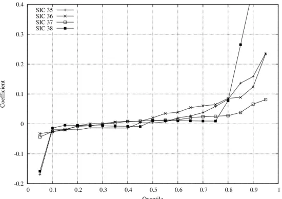
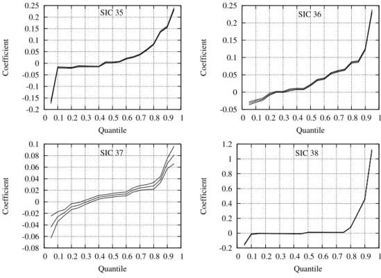
Generally speaking, the results are highly significant (see table 8). Evaluated at the median, innovativeness is observed to have a positive and significant influence for all four sectors, though the effect appears to be stronger for SIC’s 36 and 38. The median quantile however does not tell the whole story, since the coefficients vary greatly across the conditional distribution. Figure 3 shows that a similar pattern can be seen for all four sectors, and the ‘tight’ confidence intervals for the coefficient estimates in figure 4 show that the coefficients vary significantly across the conditional distribution, as one moves from the lower tail to the upper tail. For each of the four sectors, the coefficient is much larger at the higher quantiles. At the 90% quantile, for example, the coefficient of innovativeness on growth is about 40 times larger than at the median, for 3 of the 4 sectors.
The coefficients can be interpreted as the partial derivative of the conditional quantile of
y with respect to particular regressors, δQθ(yit|xit)/δx. Put differently, the derivative is
in-terpreted as the marginal change in y at the θth conditional quantile due to marginal change
in a particular regressor (Yasar et al., 2006). The evidence here suggests therefore that for high-growth firms, a larger proportion of their growth is due to their high innovativeness. This
is corroborated by the fact that the pseudo-R2’s rise at the upper extremes of the conditional
distribution. If they ‘win big’, innovative firms can grow rapidly. Conversely, there exist many firms that invest a lot in both R&D and patents that nonetheless perform poorly and experi-ence disappointing growth. Indeed, at the lowest quantiles, innovativeness is even observed to have a negative effect on firm growth. This result may at first appear counterintuitive but it
9These stock variables are calculated using the conventional amortizement rate of 15%, and also at the rate
of 30% since, as we discussed before, we suspect that the 15% rate may be too low. Due to lack of alternatives for the period under consideration, R&D spending is deflated over the three year period using the consumer price index. This choice of deflator is not ideal but we do not expect it to invalidate our results.
-0.2 -0.1 0 0.1 0.2 0.3 0.4 0 0.1 0.2 0.3 0.4 0.5 0.6 0.7 0.8 0.9 1 Coefficient Quantile SIC 35 SIC 36 SIC 37 SIC 38
Figure 3: Variation in regression coefficients over the conditional quantiles. SIC 35: Machinery & Computer Equipment, SIC 36: Electric/Electronic Equipment, SIC 37: Transportation Equipment, SIC 38: Measuring Instruments.
does in fact have a ready interpretation. As Freel comments: “firms whose efforts at innova-tion fail are more likely to perform poorly than those that make no attempt to innovate. To restate, it may be more appropriate to consider three innovation derived subclassifications -i.e. ‘tried and succeeded’, ‘tried and failed’, and ‘not tried’” (Freel, 2000:208). Indeed, unless a firm strikes it lucky and discovers a commercially viable innovation, its innovative efforts will be no more than a waste of resources.
6
Conclusion
In modern economic thinking, innovation is ascribed a central role in the evolution of indus-tries. In a turbulent environment characterized by powerful forces of ‘creative destruction’, firms can nonetheless increase their chances of success by being more innovative than their competitors. Investing in R&D is a risky activity, however, and even if an important discovery is made it may be difficult to appropriate the returns. Firms must then combine the inven-tion with manufacturing and marketing know-how in order to convert the basic ‘idea’ into a successful product - only then will innovation lead to superior performance. The processes of creating competitive advantage from firm-level innovation strategies are thus rather complex and were the focus of this paper.
Nevertheless, and perhaps surprisingly, the bold conjectures on the important role of in-novation have largely gone unquestioned. This is no doubt due to difficulties in actually measuring innovation. Whilst variables such as patent counts or R&D expenditures do shed light on the phenomenon of firm-level innovation, they also contain a lot of irrelevant,
id--0.2 -0.15 -0.1 -0.05 0 0.05 0.1 0.15 0.2 0.25 0 0.1 0.2 0.3 0.4 0.5 0.6 0.7 0.8 0.9 1 Coefficient Quantile SIC 35 -0.05 0 0.05 0.1 0.15 0.2 0.25 0 0.1 0.2 0.3 0.4 0.5 0.6 0.7 0.8 0.9 1 Coefficient Quantile SIC 36 -0.08 -0.06 -0.04 -0.02 0 0.02 0.04 0.06 0.08 0.1 0 0.1 0.2 0.3 0.4 0.5 0.6 0.7 0.8 0.9 1 Coefficient Quantile SIC 37 -0.2 0 0.2 0.4 0.6 0.8 1 1.2 0 0.1 0.2 0.3 0.4 0.5 0.6 0.7 0.8 0.9 1 Coefficient Quantile SIC 38
Figure 4: Variation in regression coefficients over the conditional quantiles. Confidence in-tervals extend to 2 standard errors in either direction. SIC 35: Machinery & Computer Equipment, SIC 36: Electric/Electronic Equipment, SIC 37: Transportation Equipment, SIC 38: Measuring Instruments.
iosyncratic variance. In this study, innovation was measured by using Principal Component analysis to create a synthetic ‘innovativeness’ variable for each firm in each year. This al-lows us to use information on both inventive input (R&D expenditure) and inventive output (patent statistics) to extract information on the unobserved variable of interest, i.e. ‘increases in commercially useful knowledge’, whilst discarding the idiosyncratic variance of each vari-able taken individually. Furthermore, while standard regression analyses focus on the growth of the mean firm, such techniques may be ill-appropriate given that growth rate distributions are highly skewed and that high-growth firms should not be treated as outliers but instead are objects of particular interest. Regression quantile analysis allows us to parsimoniously describe the entire conditional growth rate distribution, and we observed that, compared to the average firm, innovation is of far greater importance for the fastest growing firms.
In the sectors studied here, there is a great deal of technological opportunity. Competi-tion in such sectors is organized according to the principle that a successful (and fortunate) innovator may suddenly come up with a winning innovation and rapidly gain market share. The reverse side of the coin, of course, is that a firm that invests in R&D but does not make a discovery (either through missed opportunities or just plain bad luck) may rapidly forfeit its market share to its rivals. As a result, firms in turbulent, highly innovative sectors can never be certain how they will perform in future. Innovative firms may either succeed spectacularly or (if they don’t happen to discover a commercially valuable innovation) they may waste a large amount of resources. Innovative activity is highly uncertain and although it may increase the probability of superior performance, it cannot guarantee it.
Many years ago, Keynes wrote: “If human nature felt no temptation to take a chance, no satisfaction (profit apart) in constructing a factory, a railway, a mine or a farm, there might not be much investment merely as a result of cold calculation” (1936:150) - the same is certainly true for R&D. Need it be reminded, an innovation strategy is even more uncertain than playing a lottery, because it is a ‘game of chance’ in which neither the probability of winning nor the prize can be known for sure in advance. In the face of such radical uncertainty, some firms may well be overoptimistic (or indeed risk-averse) about what they will actually gain. For other firms, there may be over-investment in R&D because of the ‘managerial prestige’ attached to having an over-sized R&D department. As a result, we cannot rule out the possibility that many firms invest in R&D far from something which could correspond to the ‘profit-maximizing’ level (whatever ‘profit-‘profit-maximizing’ may mean). However, the help of economists should be at hand to provide understanding of the processes of innovation and their effect on firm performance, in order to better inform firms about what they can expect to gain from an innovation programme and bring R&D investment closer to something of a cost-benefit analysis framework. Nonetheless, there is at present but a small body of research that links firm-level innovation to subsequent performance. It would appear that linking innovation to firm performance is a research agenda that is still in need of considerable attention. This will necessarily involve ‘getting one’s hands dirty’ and working with real-world data.
References
Archibugi, D. (1992), ‘Patenting as an indicator of technological innovation: a review’, Science
and Public Policy, 19 (6), 357-368.
Arellano, M. and O. Bover (1995), ‘Another Look at the Instrumental Variable Estimation of Error-Components Models’, Journal of Econometrics, 68, 29-51.
Arundel, A. and I. Kabla (1998), ‘What percentage of innovations are patented? Empirical estimates for European firms’, Research Policy, 27, 127-141.
Bloom, N. and J. Van Reenen (2002), ‘Patents, Real Options and Firm Performance’,
Eco-nomic Journal, 112, C97-C116.
Blundell, R. and S. Bond (1998), ‘Initial Conditions and Moment Restrictions in Dynamic Panel Data Models’, Journal of Econometrics, 87, 115-143.
Bottazzi, G., G. Dosi, M. Lippi, F. Pammolli and M. Riccaboni (2001), ‘Innovation and Cor-porate Growth in the Evolution of the Drug Industry’, International Journal of Industrial
Organization, 19, 1161-1187.
Buchinsky, M. (1994), ‘Changes in the U.S. Wage Structure 1963-1987: Application of Quantile Regression’, Econometrica, 62, 405-458.
Buchinsky, M. (1998), ‘Recent Advances in Quantile Regression Models: A Practical Guide for Empirical Research’, Journal of Human Resources, 33 (1), 88-126.
Cefis, E. and L. Orsenigo (2001), ‘The persistence of innovative activities: A cross-countries and cross-sectors comparative analysis’, Research Policy, 30, 1139-1158.
Cohen, W. M., R. R. Nelson and J. P. Walsh (2000), ‘Protecting their intellectual assets: Appropriability conditions and why US manufacturing firms patent (or not)’, NBER working paper 7552.
Dosi, G. (1988), ‘Sources, Procedures, and Microeconomic Effects of Innovation’, Journal of
Economic Literature, 26 (3), 1120-1171.
Dunne, T., M. Roberts and L. Samuelson (1989), ‘The growth and failure of US Manufacturing plants’, Quarterly Journal of Economics, 104 (4), 671-698.
Engelsman, E. C. and A. F. J. van Raan (1990), ‘The Netherlands in Modern Technology: A Patent-Based Assessment’, Centre for Science and Technology Studies (CWTS), Leiden, The Netherlands; Research Report to the Ministry of Economic Affairs.
Evangelista, R. and M. Savona (2003), ‘Innovation, Employment and Skills in Services: Firm and Sectoral Evidence’, Structural Change and Economic Dynamics, 14 (4), Special Issue, 449-74.
Evans, D. S. (1987), ‘The Relationship between Firm Growth, Size and Age: Estimates for 100 Manufacturing Industries’, Journal of Industrial Economics, 35, 567-581.
Fizaine, F. (1968), ‘Analyse statistique de la croissance des enterprises selon l’age et la taille’,
Revue d’Economie Politique, 78, 606-620.
Freel, M. S. (2000), ‘Do Small Innovating Firms Outperform Non-Innovators?’, Small Business
Economics, 14, 195-210.
Geroski, P. A. (2000), ‘The growth of firms in theory and practice’, in N. Foss and V. Mahnke (eds), New Directions in Economic Strategy Research, Oxford: Oxford University Press.
Geroski, P. A. and S. Machin (1992), ‘Do Innovating Firms Outperform Non-innovators?’,
Business Strategy Review, Summer, 79-90.
Geroski, P. A. and S. Toker (1996), ‘The turnover of market leaders in UK manufacturing industry, 1979-86’, International Journal of Industrial Organization, 14, 141-158.
Greenhalgh, C., M. Longland and D. Bosworth (2001), ‘Technological Activity and Employ-ment in a Panel of UK Firms’, Scottish Journal of Political Economy, 48 (3), 260-282. Griliches, Z. (1990), ‘Patent Statistics as Economic Indicators: A Survey’, Journal of Economic
Literature, 28, 1661-1707.
Hall, B. (1987), ‘The Relationship between Firm Size and Firm Growth in the U.S. Manufac-turing Sector’, Journal of Industrial Economics, 35 (4), 583-600.
Hall, B. (2004), ‘Exploring the Patent Explosion’, Journal of Technology Transfer, 30 (1-2), 35-48.
Hall, B., A. Jaffe and M. Trajtenberg (2001a), ‘Market Value and Patent Citations: A First Look’, Paper E01-304, University of California, Berkeley.
Hall, B., A. Jaffe and M. Trajtenberg (2001b), ‘The NBER Patent Citation Data File: Lessons, Insights and Methodological Tools’, NBER Working Paper 8498.
Hall, B. H. and R. Oriani (2006), ‘Does the market value R&D investment by European firms? Evidence from a panel of manufacturing firms in France, Germany, and Italy’, International
Journal of Industrial Organization, forthcoming.
Hair, J., R. Anderson, R. Tatham and W. Black (1998), Multivariate Data Analysis: Fifth
Edition, Upper Saddle River, NJ: Prentice Hall.
Harhoff, D., K. Stahl and M. Woywode (1998), ‘Legal Form, Growth and Exits of West German Firms - Empirical Results for Manufacturing, Construction, Trade and Service Industries’,
Journal of Industrial Economics, 46 (4), 453-488.
Hart, P. E. and N. Oulton (1996), ‘The Growth and Size of Firms’, Economic Journal, 106 (3), 1242-1252.
Keynes, J. M. (1936), The general theory of employment, interest, and money, Lon-don: MacMillan.
Koenker, R. and G. Bassett (1978), ‘Regression Quantiles’, Econometrica, 46, 33-50.
Koenker, R. and K. F. Hallock (2001), ‘Quantile Regression’, Journal of Economic
Perspec-tives, 15 (4), 143-156.
Lanjouw, J. and M. Schankerman (2004), ‘Patent Quality and Research Productivity: Mea-suring Innovation with Multiple Indicators’, Economic Journal, 114, 441-465.
Lotti, F., E. Santarelli and M. Vivarelli (2003), ‘Does Gibrat’s Law hold among young, small firms?’, Journal of Evolutionary Economics, 13, 213-235.
Mansfield, E. (1962), ‘Entry, Gibrat’s law, innovation and the growth of firms’, American
Mansfield, E., J. Rapoport, A. Romeo, E. Villani, S. Wagner and F. Husic (1977), The
Pro-duction and Application of New Industrial Technology, New York: Norton.
Marsili, O. (2001), The Anatomy and Evolution of Industries, Cheltenham: Edward Elgar. Mosteller, F. and J. Tukey (1977), Data Analysis and Regression, Reading, MA:
Addison-Wesley.
Mowery, D. C. (1983), ‘Industrial Research and Firm Size, Survival, and Growth in American Manufacturing, 1921-1946: An Assessment’, Journal of Economic History, 43 (4), 953-980. Niefert, M. (2005), ‘Patenting Behavior and Employment Growth in German Start-up Firms: A Panel Data Analysis’, Discussion Paper No 05-03, ZEW Centre for European Economic Research, Mannheim.
OECD (1994), Using Patent Data as Science and Technology Indicators, Patent Manual 1994, Paris.
Roodman, D. (2005), ‘xtabond2: Stata module to extend xtabond dynamic panel data esti-mator’, Center for Global Development, Washington.
Roper, S. (1997), ‘Product Innovation and Small Business Growth: A Comparison of the Strategies of German, UK and Irish Companies’, Small Business Economics, 9, 523-537. Scherer, F. M. (1965), ‘Corporate Inventive Output, Profits, and Growth’, Journal of Political
Economy, 73 (3), 290-297.
Stanley, M. H. R., L. A. N. Amaral, S. V. Buldyrev, S. Havlin, H. Leschhorn, P. Maass, M. A. Salinger and H. E. Stanley (1996) “Scaling behavior in the growth of companies”
Nature 379, 804-806.
Sutton, J. (1997), ‘Gibrat’s Legacy’, Journal of Economic Literature, 35, 40-59.
Van Reenen, J. (1997), ‘Employment and Technological Innovation: Evidence from UK Man-ufacturing Firms’, Journal of Labor Economics, 15 (2), 255-284.
Yasar, M., C. H. Nelson and R. M. Rejesus (2006), ‘Productivity and Exporting Status of Manufacturing Firms: Evidence from Quantile Regressions’, Weltwirtschaftliches Archiv, forthcoming.