METIS: a fast integrated tokamak modelling tool for scenario design

HAL Id: cea-01873853

https://hal-cea.archives-ouvertes.fr/cea-01873853

HAL is a multi-disciplinary open access

archive for the deposit and dissemination of sci-entific research documents, whether they are pub-lished or not. The documents may come from teaching and research institutions in France or abroad, or from public or private research centers.

L’archive ouverte pluridisciplinaire HAL, est destinée au dépôt et à la diffusion de documents scientifiques de niveau recherche, publiés ou non, émanant des établissements d’enseignement et de recherche français ou étrangers, des laboratoires publics ou privés.

METIS: a fast integrated tokamak modelling tool for

scenario design

J. Artaud, F Imbeaux, J. Garcia, G. Giruzzi, T Aniel, V. Basiuk, A. Bécoulet,

C. Bourdelle, Y. Buravand, J. Decker, et al.

To cite this version:

J. Artaud, F Imbeaux, J. Garcia, G. Giruzzi, T Aniel, et al.. METIS: a fast integrated tokamak modelling tool for scenario design. Nuclear Fusion Journal of Plasma Physics and Thermonuclear Fusion, 2018, 58, pp.105001. �10.1088/1741-4326/aad5b1�. �cea-01873853�

1

METIS: A FAST INTEGRATED TOKAMAK MODELLING TOOL FOR

SCENARIO DESIGN

J.F. Artaud1, F. Imbeaux1, J. Garcia1, G. Giruzzi1,T. Aniel1, V. Basiuk1, A. Bécoulet1, C. Bourdelle1, Y. Buravand1, J. Decker2, R. Dumont1, L.G. Eriksson3, X. Garbet1, R. Guirlet1, G.T. Hoang1, P. Huynh1, E. Joffrin1, X. Litaudon4, P. Maget1, D. Moreau1, R. Nouailletas1, B. Pégourié1, Y. Peysson1, M. Schneider5 , J. Urban6

1) CEA, IRFM, F-13108 Saint-Paul-lez-Durance, France.

2) Ecole Polytechnique Fédérale de Lausanne (EPFL), Centre de Recherches en Physique des Plasmas, Association Euratom-Confédération Suisse, CH-1015 Lausanne, Switzerland

3) European Commission, Research Directorate General, B-1049 Brussels, Belgium

4) EUROfusion Programme Management Unit, Culham Science Centre, Culham, OX14 3DB, United Kingdom

5) ITER Organization, Route de Vinon-sur-Verdon, CS90046, 13067 St Paul-lez-Durance, France

6) Institute of Plasma Physics of the CAS, Za Slovankou 3, 182 00 Praha 8, Czech Republic Abstract

METIS is a numerical code aiming at fast full tokamak plasma analyses and predictions. It combines 0-D scaling-law normalised heat and particle transport with 1-D current diffusion modelling and 2-D equilibria. It contains several heat, particle and impurities transport models, as well as heat, particle, current and momentum sources, which allow faster than real time scenario simulations. This paper gives a first comprehensive description of the METIS suite: overall structure of the code, main available models, details on the simulation workflow and numerical implementation. Some examples of applications to the analysis of experimental discharges and the predictions of ITER scenarios are also given.

2

1

Introduction

Integrated modelling of burning plasmas is an essential tool for the realisation of the ITER program. For the first time in tokamak history, it is planned that any plasma experiment run on ITER must be first systematically simulated by an Integrated Modelling tool to check that the pulse is feasible, i.e. does exceed neither the physical nor the engineering limits of the machine. This tool would include a Plant Simulator and a Plasma Control System (PCS) [1] Simulator, self-consistently coupled in order to provide the most realistic simulation of the plasma dynamics as well as the diagnostics and actuator responses under the control of the implemented PCS. For modelling the plasma dynamics of entire experiments (from short after plasma breakdown to short before the plasma termination), the present paradigm is to use so-called 1.5D Integrated Modelling codes, i.e. suite of codes solving transport equations in the plasma core for energy, poloidal flux, particles, toroidal momentum in the radial direction (one-dimensional in space) using flux surface averaged quantities from 2D equilibrium solvers (in the poloidal plane). Typical examples of such codes are CRONOS [2], JINTRAC [3], ASTRA [4], PTRANSP [5], CORSICA [6], TOPICS [7], and more recently the ETS [8].

These codes integrate in a modular structure, around the core transport equations solver, various components for computing the equilibrium, source/sink terms and transport coefficients. The degree of sophistication of these components can vary, but the present trend is to use state-of-the-art modules, in particular for source terms and transport coefficients, aiming at increasing the accuracy of the simulations. This naturally has a cost in computing time, in particular when the sophisticated module is located inside the convergence loop of the core transport solver (e.g. the transport coefficient computation). Being intrinsically sequential, the workflow of such codes is difficult to parallelize. While for simulation of short experiments of a few seconds, it is tractable to use the best available modules, simulation of ITER experiments which could last up to a few thousands of seconds (hybrid or steady-state scenarios) represents a computational challenge. The multi-scale nature of the physical problem is at the origin of this challenge: plasma turbulence, which is the main cause of energy, particle and toroidal momentum transport, evolves on time scales of ~ 10-6 s, transported quantities on a time scale of ~ 1s on ITER, while the time scale for diffusion of the poloidal flux occurs on ~ 1000 s in high temperature ITER plasmas. The first-principle based transport models usually show a high degree of stiffness (the output transported flux is highly sensitive to the input temperature and density gradients) creating a numerical challenge for transport solvers. These are typically using internal time steps around 10-4 s in order to converge with such stiff transport models for the simulation of transient transport phenomena. In these conditions, the simulation of a full discharge on ITER with a 1.5D transport code using sophisticated modules typically takes a few days.

3 While this remains acceptable for detailed scenario studies, for scenario or controller scheme design one would benefit of having much faster tools that allow testing and optimising a large number of time-dependent scenarios in a computation time that allows interactive trial of scenario or controller parameters from the user. Such a tool would also be very useful to do a rapid inter-shot analysis of a plasma experiment and detect deviations with respect to an expected standard behaviour of the experiment, which could be due to an erroneous measurement or to the occurrence of a new physics phenomenon. Therefore such a tool, like the more sophisticated 1.5D plasma simulators, has applications to both prediction and analysis of plasma experiments.

This paper presents the METIS code, a fast transport simulator that has the properties described above. METIS is built on an original simplification paradigm of the transport problem, and allows realistic simulation of plasma scenarios in about 1 minute computation time, even for full ITER discharges of ~ 1000 s duration. METIS is therefore faster than real time. METIS results have supported several publications in the past years, but the description of its algorithm and models, allowing the code to be faster than real time, has never been published so far. This description is the main goal of the present paper, The METIS model is presented in section 2. Following this, details about architecture and programming languages are given in section 3 and the link to experimental databases is presented in section 4. The variety of possible METIS applications together with some detailed examples is given in section 5. Appendices provide a detailed description of the source models.

2

Physical model

To be faster than 1.5D codes, one has to simplify the physics model. This means a priori less reliability of the prediction, i.e. one would expect that the overall result of the simulation deviates more from a real experiment. In order to keep the reliability of the simulation results one has to carefully establish what are the aspects of the transport that can be modelled in a simpler way. Here the underlying principles for the METIS design have been the following: keep the 1.5D paradigm on what can be reliably modelled with accuracy (typically: plasma equilibrium and resistive current diffusion). Use a much simpler, quasi-0D approach for what is usually modelled with less reliability even by sophisticated models in the 1.5D paradigm (typically: turbulent transport). Keep in the model the non-linear interactions between the transported quantities, plasma equilibrium and source terms, in particular the key phenomenon for fusion reactors that is the self-heating via the fusion-born alpha particles. Keep in the model a realistic modelling of the dynamic character of the sources and plasma response, because we are aiming at realistic time-dependent simulations. We describe now the details of how these principles are practically implemented in METIS.

4

2.1

Plasma equilibrium and current diffusion

Among the quantities simulated by core transport codes, the plasma current density is the one that is most accurately predicted in a large variety of experiments. In the absence of magneto-hydrodynamic activity, the neoclassical resistivity seems a valid diffusive model to describe resistive current diffusion in tokamak experiments, at least during the flat-top phase of the H-mode [9]. Therefore in METIS current diffusion and plasma equilibrium computations are fully kept in the 1.5D paradigm: i) a 2D equilibrium code is run periodically to update the metrics of the poloidal flux transport equation in a way consistent with the plasma pressure and current profiles; ii) the 1D poloidal flux transport equation is solved with all its terms.

The current diffusion equation is solved in terms of the poloidal flux Ψ, on a uniform toroidal flux coordinate ρ grid, exactly as in the CRONOS 1.5D code [2]:

= 〈|∇ | 〉 ∥ 〈 〉 + 〈|∇ | 〉 ∥ 〈 〉 〈|∇ | 〉 ! + #_# + $% #% # & + % ∥'〈 〉 ()* (1) where norm

t

∂

∂

Ψ

is the time derivative of the poloidal flux at a given radial position +_),-., /_∥ denotes the parallel conductivity (calculated following the Sauter model [10]), F is the diamagnetic function,

jni the current density driven by the non-inductive sources, R the major radius,

µ

permeability of free space, (4π×10-7

in MKS units), +_. the value of ρ at the last closed flux surface, and the normalised toroidal flux coordinate

m norm

ρ

ρ

ρ

ρ, i.e. in an elementary volume dV enclosed between two magnetic surfaces distant of dρ. We remind the definition of the toroidal flux coordinate,

0

B

π

ρ

=

Φ

the vacuum magnetic field at a given major radius R0 (usually taken at the centre of the vacuum

vessel). The normalised radial grid does not depend on time, but ρm is time-dependent and calculated

by the equilibrium solver.

Solving the current diffusion in the same way as the traditional 1.5D integrated modelling code is not a drawback from the performance point of view since it corresponds to the transport phenomenon with the longest time scale. To speed up the calculation, current diffusion is calculated on a 21 points radial grid only and the 3-moments description (Shafranov Shift, ellipticity and

5 triangularity) is used for the MHD equilibrium [11,12]. The last closed flux surface (LCFS) can be either described by moments or as a series of (R,Z) points. In this last case an additional morphing (continuous deformation) is applied to flux surfaces to match the LCFS with effect weighted as:

+01, 34 = +.,.5) 01, 34 601 − 15 4 + 15 9:;<_{> ?}0=4_0@,=4A (2)

Where +_.,.5) 01, 34 is the moment description of flux surfaces (1 is the radial coordinate described in next section and 3 is a poloidal angle); +_{BC D}034 is the LCFS poloidal representation given as a series of (R,Z) points; +_.,.5) 01, 34 is the LCFS described by moment and E_. is an arbitrary parameter. The value E_. = 5 is typically used, as it has been found to minimize the discrepancy for geometrical coefficients involved in the current diffusion equation (1) for various devices (JET, Tore Supra, JT-60SA, ITER) and scenarios, with respect to equilibria calculated using the HELENA code [13]. The value of this parameter is kept tunable by the user.

2.2

Radial coordinate

For the description of all radial profiles, METIS uses a uniform 21 points grid on the normalized minor radius x, defined as follows: for each magnetic surface, the minor radius is defined as G =H.IJKH.*)_$ , where Rmax (resp. Rmin) is the maximum (resp. minimum) major radius of that

surface. The minor radius is then normalized to its value at the LCFS am, so that 1 = I I .

In H-mode, the top of pedestal, located at 1_L5# is always set in METIS at the second point from the edge. The internal grid of METIS is 1_M =I_$N0O − 14 with O an integer between 1 and 21 and 1_L5#= 1$N. Therefore, the width of the pedestal is always 5% of plasma minor radius. Use of a simple grid with fixed step simplifies the numerical computation. This technical choice typically overestimates the pedestal width which is about 2-3 % of the minor radius in present experiments, but this has a very limited impact on the profiles predicted by METIS, which are based on scaling expressions for the energy content of core plasma and the pedestal (so they are not gradient based, see the section below). We have checked that with a width of 5 % we have about the same amount of bootstrap current (the difference is less than 5%), integrated on pedestal width in METIS than with a pedestal width of 2-3% in CRONOS simulations.

2.3

Heat transport

The transport of energy in the core of tokamak plasmas is dominated by turbulence. In spite of enormous efforts and progress made by the fusion community to understand and predict plasma turbulence, the prediction of the resulting transport flux still features large uncertainties. First-principle gyro-kinetic codes are extremely expensive in terms of computing resources so that they can barely be applied to the long-time scales of plasma experiments. On the other hand, the existing reduced models

6 (e.g. GLF23 [14], TGLF [15], Qualikiz [16]), even when first-principle based, fail to capture completely the complexity of the turbulence phenomena and their predictions are in some cases quite far from the experimental results. This is particularly true for plasmas at high beta and a significant fraction of energetic particles, where non-linear physics becomes dominant [17, 18], but also for H-mode plasmas where the fusion performance is fully dominated by the height of the pedestal which is still far from being predicted reliably. We touch here the main paradox of present Integrated Modelling, which is that the largest source of uncertainties lies at the heart of the problem solved, namely the prediction of the heat and particle fluxes. Moreover, the reduced “first-principle based” models usually feature strong dependences on the gradients of the transported quantities, which requires using rather small time steps in the transport solver (typically ~ 10-4 s) if one wants a numerically accurate resolution of the transport dynamics. This numerical constraint makes this type of models difficult to apply to simulate a full ITER discharge lasting several hundreds of seconds. This is even more difficult in view of scenario optimisation studies where it is desired to test several combinations of actuators, e.g. power, timing and parameters, hence requiring a large number of these long simulations and some manual trial and error process.

Therefore simplifying the heat transport modelling assumptions, which are both the largest source of uncertainty and the largest CPU time consumption in a classical 1.5 D integrated modelling simulation, is an effective way of increasing the performance with the smallest impact on the reliability of the results, in view of a fast scenario simulator. In METIS, heat transport is treated in a mixed 0D – 1D approach in two steps, by separating the time and radial dimensions. This approach is found to be quite successful for simulating the main dynamics of the core plasma temperature profiles, although it naturally has limitations for phenomena in which spatial and temporal evolutions are coupled: for example, details of heat pulse propagation following a pellet injection cannot be resolved and would require using a classical 1.5D solver.

The first step consists in solving a time-dependent 0D equation for the plasma thermal energy content Wth:

#P?Q

# = − P?Q

RS + TU,VV (3)

In this ordinary differential equation scaling expressions for the energy confinement time τE are

typically used, a multi-machine approach widely used for extrapolating present results to future tokamaks such as ITER [19]. Although this approach has inherent limitations when non-linear physics is dominant, it is still valid for a significant class of future plasmas [20]. Ploss represents the total power

transported through the plasma separatrix by diffusion or convection mechanisms (detailed expressions are given in appendix 8). Multiple scaling expressions are coded in METIS for calculating the value of τE in a self-consistent way with the actual parameters. The expression of Wth actually

7 depends on whether the plasma is in L or H mode. This information, as well as the ability to handle L-H and L-H-L transitions, is of course essential for a full scenario simulator such as METIS. The list of available scaling expressions is of course easily extensible and could cope with e.g. new scaling laws based on the future analysis of the ITER shot database, in order to make METIS even more useful for ITER operation.

The METIS code uses scaling expressions of the L-H power threshold to deduce whether the plasma is in L or H mode. Multiple options are available from the literature and new ones can be easily added. When in L mode, no pedestal is created and an L-mode scaling expression is used for τE in equation 3.

When in H mode:

• A pedestal is created. Its height can be prescribed in multiple ways (constant or scaling expression).

• An H-mode scaling expression is used for τE in equation 1.

By default, the L-H transition is modeled as an immediate change of the value of τE in equation 1.

Nevertheless in experiments, the transition from L to H mode is not abrupt when crossing the power threshold. There is often a Ploss range slightly above the threshold Pthreshold that yields an intermediate

confinement level. This can be mimicked in METIS by defining a linear transition in _W WX YY

?Q >YQ XZ

between the L and H mode energy confinement scaling expressions. A detailed explanation about how Ploss is calculated is given in the appendix.

The second step consists in calculating the electron and ion temperature profiles, assuming steady-state transport equations and purely diffusive transport, the heat flux at a radial position x can be expressed as: [> J

=

=

[> J

=

=

where Qe and Qi are the sum of all the electron and ion heat source terms, including the equipartition

term Qei. The diffusion coefficients for electron and ions are noted respectively f5 and f*. The

conductivity coefficients for electron and ions are noted respectively g₅ and g_* (linked to diffusion coefficients by : g_5,*= _5,*f_5,*). The geometrical coefficient h^is the derivative of the plasma volume

8 enclosed in a magnetic surface with respect to the normalised minor radius x, while 〈∣ i+ ∣$〉 is the surface average of the squared gradient of the toroidal flux coordinate. We note that although the temperature profiles are solved using steady-state equations, the dynamics of heat transport can still be accounted for by the first equation (on the global energy) which is time-dependent and used to normalize the heat conductivities g₅ and g_*(or alternatively the diffusion coefficients f₅ and f_*). Validation against experiments shows that this approximated approach is relevant for the description of transient phenomena at the scenario level (e.g. transport dynamics during current ramps). Note also that with this formulation, the temperature profiles calculated by METIS take into account the information on the radial distribution of the heat sources.

To complete the second step, the diffusion coefficients used in the equations (4) must be calculated in a way consistent with the energy content that has been calculated at the first step. This is done differently in L and H mode.

In L-mode:

i. The dependence of the electron diffusion coefficient on plasma parameters or on the radial coordinate is prescribed. Multiple options are coded in METIS and new expressions can be easily added. Three widely used options are a) Bohm-gyro-Bohm model [21,22] b) fixed radial dependence of the type f₅= f_N(1 + λ1k); where λ and l are constants chosen by the user (the default values are λ = 3 and l = 2 , or c) f₅= f_Nok(1) ; where q is the safety factor and l is a constant chosen by the user.

ii. The ion diffusion coefficient is calculated from the electron one with a simple expression of the type: f_* = p_5,*f₅. Often p_5,* is prescribed to be a constant, but it can also be provided by other analytical expressions [23-26]

iii. Steps i and ii yield the radial shape of the diffusion coefficients and their relative value. The coefficients are then normalized in such a way that the thermal energy content obtained from the integral of the pressure profile corresponds to the value calculated from equation 1, i.e. q

$\ ( 5r5+ *r*)h′ @

JtN u1 = vw. In order to have an exact (inverse) proportionality relation between the normalization factor of the diffusivities involved in equations (4) and the energy content, the contribution of the boundary conditions r_{5,BC D} and r_{*,BC D} to the integral must be removed. Indeed equations (4) define only the temperature gradient, therefore the temperature profiles are defined as r(1) = r_{BC D}+ \_@J [_Ju1, in which only the second term is inversely proportional to the diffusivity. The contribution to the integral of a finite LCFS temperature represents an energy content v_N =q_$\ (_JtN@ ₅r_{5,BC D}+ _*r_{*,BC D})h′u1 . The normalization

9 constant of the diffusivities is therefore calculated following the relation q_$\ (_JtN@ ₅\_@J [_J>u1+

*\_@J [_Jdu1)h′ u1 = vw− vN.

To complete step 2, a convergence loop on the temperature profiles resulting from this process is performed in order to find the self-consistent value of the equipartition term Qei in equations (4),

which is proportional to Te − Ti.

In H-mode, the procedure is similar to that of the L mode, with the only difference that the pedestal top is used as the boundary condition for the integration of equations (4). A scheme of such a procedure is shown in figure 1.

Figure 1: Calculation of the plasma energy content. The energy is decomposed between offset (W0), pedestal (Wped) and core (Wcore).

2.4

Electron density profile

Particle transport is also dominated by turbulence, however the level of understanding is lower than that for heat transport. The existence of significant inward and outward pinches which in turn depend on the accurate description of turbulence requires a significant amount of computational time if a first principle approach is used. Additionally, unlike for heat transport, the sources uncertainties are significant close to the pedestal region. On the other hand, a significant amount of work has been performed in order to characterize some density features, as the peaking, by analysing extensive plasma tokamak databases [27]. In METIS, an approach that is even simpler than for heat transport is chosen, based on the prescription of some quantities.

10 The primary quantity for determining the density of the plasma species in METIS is the electron density profile. It is described by 3 parameters, which can vary with time:

i. the line-averaged density (x₅), which is prescribed

ii. the peaking factor _〈)〉) which is either prescribed or computed with the help of a scaling expression (to take into account self-consistent dependencies on plasma parameters, various options from the literature are available, with one set of scaling expression for L-mode and another one for H-mode)

iii. the density value at the separatrix ( _5,I) obtained from simple models or scaling expressions depending of the plasma configuration: poloidal limiter, toroidal limiter, axisymmetric divertor with X-point. In the last case (X-point) the expression depends also of the confinement mode L or H.

In L mode the shape of the profile is defined as:

50y, 14 = 0 5,N0y4 − 5,I0y4401 − 1$4z 0 4+ 5,I0y4 (5) where {₎=)>_〈)0 ,JtN4

>〉0 4 − 1.

In H mode, in order to ensure that the pedestal is also present in the electron density profile, the density profile is computed by another method. The density profile is constrained by the line-averaged value, the peaking factor, the constraint of flat profile at the centre, the edge value and the constraint that the temperature profiles are strictly monotonically decreasing. A piecewise cubic Hermite polynomial interpolation is used to compute the profile, calculating the pedestal density that fulfils those 4 constraints: the electron density is given at 3 points: at the centre (x=0), at the top of the pedestal (x= 0.95) and at the edge (x= 1) with the constraint of null derivative at the centre. The value at the top of the pedestal is computed as the maximal value ensuring negative derivative of electron temperature (with a minimum of 0.01 ~r_5,N− r_5,I• )

2.5

Post-processing of temperatures and electron density with neural

network based models

From the results of an initial METIS simulation, it is possible to compute as a post-processing the electron temperature, ion temperature and electron density using more sophisticated transport models than the scaling-based ones. For this post-processing duration to remain of the same order as the one of the main METIS computation, neural network based models such as Qualikiz-NN should be used, which are approximations to quite sophisticated transport models [28]. This allows comparing the prediction of such more physics-based transport models to the scaling based-ones. In this calculation, the steady-state transport equation is solved from the top of the pedestal to the magnetic axis and keeping the sources, current density profile and equilibrium from the result of the initial METIS simulation. The steady-state solution is thus calculated for each time step using physics-based transport models. However, in order to keep a fast computation time, this is at the expense of losing the self-consistency between transport, equilibrium, and sources.

11

2.6

Ion species

In METIS, all ion species density profiles are assumed to be proportional to the electron density profile, with exceptions of the tungsten species and helium ashes, which have specific treatments (see Appendix 10.1 & 10.2). Alternatively to this simple assumption, one can use a simple neoclassical model based on impurity shielding/accumulation, similar to that one used for tungsten. However in practice this model is not frequently used, as turbulent transport remains generally dominant over the neoclassical one for light impurities.

The user also specifies the reference effective charge (line averaged) for the plasma Zeff,ref , which is

either prescribed as a time-dependent value or self-consistently calculated from a scaling expression. This value is called “reference”, although it is used as the exact effective charge of the plasma when the main plasma species are H, D, He. A correction is applied in the case of D-T mixture to account for the presence of €_5,IVw5V resulting from the D-T fusion reactions and in case of presence of tungsten impurity. It thus represents the effective charge in absence of €_5,IVw5V and tungsten.

Then, various types of plasma compositions, which have to be consistent with Zeff,ref , can be prescribed

by the user. METIS first calculates their volume average densities, from the rules explained below, then applies the radial profile option (by default: same profile as the electron density) to these average densities.

METIS distinguishes the following types of ion species:

• Main species: can be H, D, D-T mixture, or He. In case of a D-T mixture, the user prescribes the isotopic density ratio _〈•〈•‚〉

ƒ〉 and a specific treatment is applied for the Helium density (see

section 10.1)

• Minority species: in case of Ion cyclotron Resonant Heating (ICRH) minority heating, the user can specify the type of one minority species (H, D ,T, He3 and He4 ) and the average density ratio of the minority species with respect to the main ion species

• Impurity species: two additional impurity species can be included, the user specifies their type as well as their relative average density ratio 〈•_〈•d „, 〉

d „, 〉

• Optionally, the tungsten species can be added. It is treated separately, self consistently with the divertor to provide feedback on the tungsten source (see section 10.2).

Computation of the ion densities

The specification of the plasma composition and the average density ratios as described above, together with the effective charge and electro-neutrality constraints, provides a linear system with equal number equations and unknowns and thus allows calculating the average density of all ion species.

The final value of the effective charge is computed with the whole set of profiles including helium ashes and tungsten.

12 In the presence of Helium ashes or Tungsten impurity, the effective charge is modified and become:

…5††(y, 1)

= ‡(y, 1) + ˆ(y, 1) + [(y, 1) + 4 n‡5(y, 1) + …*.L,@$ *.L,@(y, 1) + …*.L,$$ *.L,$(y, 1) + …P,I‹5-IŒ5#$ ~r5(y, 1)• P(y, 1)

5(y, 1)

(6)

Verifying (in case of D-T plasma):

5(y, 1) = ‡(y, 1) + ˆ(y, 1) + [(y, 1) + 4 n‡5(y, 1) + …*.L,@ *.L,@(y, 1) + …*.L,$ *.L,$(y, 1) + …P,I‹5-IŒ5#~r5(y, 1)• P(y, 1) (7)

With _{*.L,$ t} 〈•_〈•d „, 〉

d „, 〉 *.L,@ , [ =

〈•‚〉

〈•ƒ〉 ˆ and ‡ = •.*) ˆ

For other main ions choice the formulation is updated as follows:

• Hydrogen main ion: if the minority species is not deuterium _ˆ= 〈•‚〉

〈•ƒ〉 ‡ and [ = 0,

otherwise _ˆ= Ž〈•‚〉

〈•ƒ〉+ •.*)• ‡ and [ = 0,

• Helium main ion: _ˆ= _‡= _[ = 0 ; if ICRH minority heating scheme using H, D or T then _‡,ˆ,[ = •_{.*) ‡5}

2.7

Plasma rotation

An estimate of the rotation is carried out in METIS, mainly taking into account the effect of neutral beam injection and intrinsic rotation. Simple models are used to handle toroidal rotation due to parallel electric field and lower-hybrid current drive (LHCD). The effect of ripple losses is only taken into account for Tore Supra, device for which a scaling exists [29]. The toroidal rotation due to fast ion losses and to fast ion momentum transport are not taken into account, because there is no simple model available for these. No feedback of the rotation on the standard confinement is taken into account. Toroidal rotation only impacts the ITB formation.

The simple model implemented in METIS is sufficient for the study of Neutral Beam Injection (NBI) dominated plasmas, as well as for reactor studies, in which the fast alpha distribution is close to be isotropic and does not allow to transport a significant part of toroidal momentum [30]. This simplified model does not allow studying plasma rotation when the plasma is heated mainly by Ion Cyclotron Resonant Heating (ICRH), when ripple is significant on other devices than Tore Supra, or when the confinement of fast particles is poor (i.e. when the fast particle orbit size is comparable to the minor radius of the plasma).

The computation of rotation in METIS is separated in three parts. The first part consists in the evaluation of the volume-averaged toroidal momentum. The second part consists in the evaluation of rotation at the LCFS. The third part consists in the computation of the radial profiles of toroidal and poloidal rotation velocities and finally of the radial electric field.

13 general discussion can be found in [31]. The total momentum is defined as:

•, = \ ∑_N@ M∈—VL5˜*5V™’L“M M•”•,Mh^u1 (8)

where ”_•,M is the toroidal velocity of the species k, ’_L the proton mass, “_M the number of nucleons of the species, _M the species density, • the geometrical major radius of the flux surface. With this approach, the contribution of electrons is neglected because of their negligibly small mass.

The evolution equation of •_, is: #H? ?

# = − H? ?

Rš + ›•,œ%•+ ›•,V5U†+ ›•,H + ›•,ž∥+ ›•,-*LLU5+ Ÿ),N (9)

where the toroidal momentum confinement time _• is assumed to be related to the energy confinement time _ž (see below for details) and includes the friction of the plasma with neutrals at the edge. From •, we deduce the volume-averaged plasma rotation ¡_• =_¢H? ?

šH£`dY with ¤• is the conversion factor

between velocity and momentum:

¤• =_{〈‹š,YQ£„>}@ _〉\ ∑_N@ M∈—VL5˜*5V™’L“M M•”•,VwIL5h^u1 (10)

and 〈”_•,VwIL5〉 = \ ‹š,YQ£„>]

¥ _#J

\ ]¥_#J

with ”_•,VwIL5 is the profile of toroidal rotation as described below (assuming that all species have same rotation shape profile) and •_IJ*V the center of each flux surface.

Momentum sources are due to:

1. Neutral beam injection toroidal moment source :

›•,œ%•= ∑²∈—‡,ˆ,[™’²\ •_N@ IJ5014L³´µ,¶_5ž¶0J4·$5ž_.¶¶ p²014h^014u1 (11)

With •_IJ5 is the magnetic axis of each flux surface; ¸_œ%•,²014 is the profile of power deposition due to NBI ; p_²014 is the profile of pitch angle (p = ‹_‹∥); ’_² is the mass of injected species; ¹_²N is the injection energy in eV and e the electron charge.

This expression implies momentum conservation, which is true if fast ion losses are negligible. 2. The intrinsic plasma toroidal rotation source is:

›•,V5U† =¢š ºš,Y>X»_Rš (12)

The intrinsic plasma rotation ”_•,V5U† is given by a scaling law time a factor: ”•,V5U†= ¼*) -*)V*˜ ”•,V˜IU*)Œ (13) Where ”_{•,V˜IU*)Œ} is either:

• Rice scaling is taken from [32] :

”•,V˜IU*)Œ = 0.4610@@¾-5†@.@T•@.N¿LK@.À•-5†$.$ (14) T• = 2〈Er*∑M∈—VL5˜*5V™ M〉 +$_q0PKP_]„?Q4 (15)

14 This expression for T_• takes into account the fact that for dominant electron heating the spontaneous toroidal rotation changes only because of ion pressure increased. On JET it was found that for NBI heated plasma, the thermal pressure is close to two times the ion pressure.

• Barnes and Parra scaling [33] for which we have taken Δr_* = 〈Wd 〉 〈)d 〉

• deGrassie scaling [34] for which we have taken Âr_* = 〈W_〈)d 〉

d 〉 .

This definition of Âr_* is the best generalization of the experimental measurement used in papers that can extend the implementation of the formula to METIS.

The factor ¼_{*) -*)V*˜} is either provided by the user or computed using the model described in [35]. 3. RF driven rotation source terms:

This source term correspond to the toroidal moment transferred from RF waves to the plasma [36]: ›•,H = − 02 ÃB‡− 14 H >»_˜ )∥, TB‡, w− ÄžCCˆ H_{$ ˜}>» TžCH‡ (16)

Where Ã_B‡ is the directivity of LH wave. The parallel refractive index of the EC wave is assumed to be near the optimal value to maximized current drive efficiency (Ä_5˜˜#~0.5) •_-5† is the geometrical center of the plasma ( •_-5†= H £` _$KH d ).

4. Rotation source due to parallel electric field:

This term is negligible during flat-top but important during ramp-up and also because it breaks the symmetry between co and counter current [37]. This term reads:

›•,ž∥= .> 5 .„ ¢š Rš Æ>»» Ç>»» •ÈÉ•Ê 〈)>〉 D„ (17)

Where Ë_5†† is the effective mass of the plasma; ¿_Ì the ohmic current and ¿_-Í) the electron runaway current; 〈 ₅〉 is the volume averaged electron density and ›_L the plasma poloidal surface.

5. Friction on cold neutral:

At the edge of the core plasma, the rotation is slowed down by the friction with cold neutrals coming from recycling and gas puff. The main contribution comes from charge exchange between cold neutrals and plasma ions. This term reads:

Ÿ)N= − ’L\ ~∑_N@ M∈—‡,ˆ,[™“M M •〈/”〉˜J•IJ5”• Nh^u1 (18)

where _N is the density of neutral hydrogen isotopes (see. Appendix 7.11), 〈/”〉_˜J the rate for charge exchange reactions. This factor is implemented only for H/D/T plasma.

The confinement time of toroidal rotation is observed to be a fraction of the energy confinement time [38, 39] and often close to the ion confinement time:

15 With _** = 5 \ )d[d]

¥_#J

\ ~_dÉ _>,d•]¥#J and ¼R,-, is an adjustable factor of order of one.

Usually, the edge value of plasma rotation is far from being null. We use a simple model to determine it assuming there is no friction with the SoL and the only damping term is the friction with neutrals. Additionally, we assume that momentum is purely convective at the edge. The edge rotation reads:

•, ,5#Œ5=ŽDš,³´µ∑_{Ñ∈—Y„>Òd>Y™}ÉDš,Y>X»_{ÐÑ Ñ}É Dš, ;ÉDš,S∥É Dš, d„„X>• ∑_{Ñ∈—Y„>Òd>Y™ÓÑ Ñ} .„ ) Ê? H>»K ,

(20)

where _,Í is the flux of ions exchange through the LCFS that contains contributions from interchange, cold neutral fuelling, pellets fuelling and neutral beam injection:

,Í =$_Ô\ ~ÕÖ+ ÕEÖ•h ′_u1 1 0 5 [d,£ + D Çx + ›L5UU5 + W³´µ 5ž¶ (21)

The first term in RHS of equation 21 is, in most of cases, the main contribution to _,Í ; others terms being negligible. Nevertheless, with only this first term, the prediction of edge rotation can become unphysical during early ramp-up phase and during some transients. To prevent this to happen, terms taking into account particle sources have been added.

The third part of this calculation consists in an estimation of the radial electric field ¹_-(1), poloidal (h_=,*.L) and toroidal (h_•,*.L) rotation of the main impurity, in the plasma equatorial plane (Z=Zref) at the low field side. We assume that the toroidal angular rotation ¡_•(1) is homothetic to a chosen kinetic profile (usually the ion temperature, which has been found to be a good proxy for h_•,*.L in JET NBI-dominated experiments) and preserves •_, with boundary condition edge value given above. By using formula (8.22 & 13.1) from [40], weighting it with mass and density and summing on all species and flux averaging it (see reference 2), we are able to compute the radial electric field from ¡•(1) , pressure gradients and poloidal rotation estimation (h=,M= ×M¾=):

¹- = Ø¡•#_# +_{∑Ñ∈—Y„>Òd>Y™}@ _.Ñ)Ñ∑M∈—VL5˜*5V™Ž._ÇÑÑ#([_#d)Ñ)− ’M M×MŸ 〈_H@〉#Ù_# • Ú 〈|∇+|〉 (22) The poloidal rotation (h_=,M) is estimated using either:

• The Kim formulation [37] that provides the poloidal rotation in a plasma composed of one main ion and one impurity

• Assuming no friction between ion species and using the formulation from reference [41] • Assuming all ion species have the same toroidal rotation

• Assuming solid plasma rotation, i.e. h_=,M = 0

To compute the toroidal rotation (h_•,*.L), we applied equation 15 in the reference [2].

16 METIS includes fast solvers for the computation of the source terms for the current diffusion equation (1) and the heat transport equation (4-a, 4-b), where electron and ion energy sources are distinguished. A source term is a radial profile which is also time-dependent and evaluated at each time slice of the METIS simulation. The source terms are also recalculated at each step of the global convergence scheme in order to obtain a self-consistent solution. Therefore, the source modules are chosen to be fast and simple enough to avoid impeding the overall computation speed of METIS. Particle and toroidal momentum profiles being not calculated from the usual transport equations, they do not require the calculation of “source terms” in the classical definition: the external input of particles and toroidal momentum are treated differently (see sections 2.4, 2.6 and 2.7).

The source terms of the transport equations can be either prescribed as time-dependent radial profiles or calculated consistently with the simulated plasma characteristics. The source modules calculate also (when relevant) the neutron rate due to fusion reactions (either from thermal or energetic ions), as well as the fast particle pressure (parallel and perpendicular to the magnetic field) due to the heating scheme. Those quantities are not directly involved in the transport equations, though the fast particle pressure contributes to the total pressure and thus enters the equilibrium calculation as an input. They are however very useful quantities for comparison of the simulation to an experiment and data consistency applications (neutron production, stored energy) as shown for JET [42].

Several source terms have been included in METIS such as NBI, ICRH, Lower Hybrid (LH), Electron Cyclotron Resonance Heating (ECRF), pellets, fusion reactions of thermal ions, ripple effects, ionisation from wall recycling/gas puffing, radiative processes. In general, a simplified description is used for each source term which, on the other hand, is sufficient to have a first evaluation on their impact on the main plasma characteristics. A detailed description of the different sources is given in the appendix.

3

Numerical algorithm

METIS is coded mostly in MATLAB language and contains some mexfile in C and FORTRAN allowing to speed-up the computation (for interpolation and PDE resolution).

17

18

3.1

Global convergence in time and non-linearities

A key challenge in plasma physics is the strong non-linear coupling between plasma profiles, transport coefficients and source terms of transport equations, as sketched on figure 2. In classical 1.5D integrated modelling codes, in order to take accurately into account these non-linear couplings, a convergence loop is usually carried out at each time step, which is very expensive in terms of CPU time. In METIS, in order to use large time steps and aiming at a fast Plasma Simulator, an original numerical algorithm has been developed, similar to a waveform relaxation algorithm [43]. It consists on a global convergence loop on the whole time evolution of all plasma quantities, noted gN at iteration

N. At each iteration of this main loop, a new time evolution of all plasma quantities F(gN) is calculated

in a step-by-step update (starting from the gN time evolution) of the quantities involved in the transport

equations. This new time evolution F(gN) is then combined to the one of the previous iteration via an

oscillation damping scheme (to ease the global convergence), providing the resulting time evolution at iteration N+1:

ÛœÉ@= Üœ Ÿ(Ûœ) + (1 8 Üœ4Ûœ (23)

Where Ü_œ is an oscillation damping coefficient varying with the iteration number. We use ÜœÉ@ 0.95 Üœ for the 21 first iterations and ÜœÉ@ 0.3 Üœ afterwards. The maximum number of iterations is set to 31. The loop terminates when the relative change between Ÿ0Û_œ4 and gN falls below

a requested value (10-2 in “coarse” computation mode and 10-3 in “detailed” computation mode). Additionally, to be able to solve ODE and PDE for any time step size, METIS uses, for time integration, an exponential integrator solver [44,45]

3.2

Graphical user interface

The METIS code can be used from command line or through a graphical user interface (GUI). This GUI makes the code user-friendly and allows to parametrize and run simulations in an easy way. The GUI provides also predefined graphics and a generic tool to browse and plot data.

19 Figure 4: METIS data browser windows

4

Link to tokamak databases, infrastructure and other codes

4.1

Reading input data from experimental databases

When doing simulations based on existing experiments, several plasma measurements are used to prepare the input simulation file. The access to experimental databases is handled by tools included in METIS and usable through the METIS GUI. The database access is however decoupled from the simulation itself: it is done entirely before the run. After database access, any signal can be edited and modified using the METIS GUI.

The access to experimental databases is done via a tokamak dependent routine which maps the database variables onto the METIS data structure. For some of the tokamaks already coupled to METIS (JET, TCV) database access is done via MDS. WEST and Tore Supra data access is done using the local TSLib library and the ITER Integrated Modelling Analysis Suite (IMAS) [46]. METIS is also integrated in the Integrated Tokamak Modelling (ITM) suite of codes [8]. METIS allows also for WEST and Tore Supra to perform pre-shot simulation by means of direct access to the Plasma Control System (PCS) configuration data. For COMPASS, METIS uses a local mechanism to read the database. For other tokamaks (DIII-D and EAST), data preparation is based on a dedicated pre-processing tool. Data access routines also apply specific default simulation parameters for each machine. Additionally, for future machines such as ITER, DEMO or JT-60SA, METIS GUI includes a

20 dedicated scenario generator allowing an easy preparation of scenario template. METIS is also delivered with a set of reference simulations for JT-60SA and for WEST.

METIS input data are made of the following waveforms:

• boundary condition for the current diffusion equations (plasma current or poloidal flux at LCFS)

• injected power for heat sources • effective charge

• line-averaged density

• plasma geometry (either moments or LCFS points). • isotopic plasma composition ()₎‚

Z) for reactor plasma

• confinement enhancement factor • isotopic composition of NBI (_ÞÞ‚

ƒ for reactor plasma or

¢ß

¢ƒ for standard plasma)

and scalar parameters describing internal physics model configurations, sources configurations and numerical scheme configuration (about 200 parameters).

Additionally, METIS internal data can be constrained by experimental data or data computed by other codes. METIS can use external data for: electron density, electron and ion temperatures, toroidal rotation, any additional heating (the shape of deposition are renormalized to the prescribed input waveform), line radiation, Zeff (profile) and runaway electrons current.

4.2

Link to IMAS and CRONOS

Originally METIS has been conceived as a module of the CRONOS [2] suite of codes. Later METIS became an autonomous code and was further developed. The present version still preserves the link with CRONOS that allows preparing a METIS simulation using CRONOS data, comparing METIS results to CRONOS results and converting a METIS data set into a complete CRONOS data set. All this can be performed through the GUI of METIS and CRONOS. Additionally, METIS can use CRONOS data (for kinetic profiles and sources) instead of his internally computed data.

METIS is also completed link with the IMAS infrastructure (and on the same way with WPCD EUROfusion infrastructure, that is very similar to IMAS one). METIS can read in input simulation through UAL (Universal Access Layer) and wrote is results in IDSs (equilibrium data, kinetic profiles, all sources and many other data). METIS can be run as a standalone code in IMAS infrastructure or as an embedded actor inside a KEPLER actor.

5

Some applications of METIS

Since METIS is basically an integrated transport solver with simplified assumptions and treatment of some of the transport equations, it can be used for most applications of classical integrated transport suites, providing a first and faster but yet meaningful alternative to such suites.

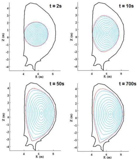
21 A predictive simulation of the ITER hybrid scenario is presented here in order to illustrate the typical quantities that are produced by METIS. The scenario addressed in this simulation is the ITER hybrid scenario assisted by ECCD previously simulated by CRONOS and presented in Ref. [47]. For a given LCFS (analytically prescribed or computed by a free-boundary equilibrium code), METIS can predict the plasma equilibrium evolution from the initial phase (post-breakdown) to the flat-top (and eventually the ramp-down phase too). This is illustrated in Fig. 5, where poloidal plots of the flux surfaces are shown at 4 different times.

Figure 5: METIS simulation of ITER hybrid scenario: snapshots of computed equilibrium evolution, from the ramp-up phase to the stationary flat-top phase. The thick black curve represents the ITER first wall, the red curve

is the LCFS (assigned as an input in this simulation)

The results of the simulation can be examined by plotting many different quantities. In addition to the 2-D equilibria shown in Fig. 5, time evolution of 0-D or space-averaged quantities or radial profiles of space-dependent quantities at given times can be displayed. An example of the former is shown in Fig. 6, where plasma current, central density and Q factor (defined as the ratio of fusion to additional heating power) are plotted vs time in the top panel, and the various powers that heat the plasma are plotted in the bottom panel. Note that plasma current and additional heating powers are input waveforms of the simulation, whereas central density, Q factor and alpha power are computed outputs of METIS. Computed profiles are shown in Fig. 7 at different times: safety factor (left) and electron temperature (right). Note that the q profile is still slowly evolving after 500 s and finally attains the flat

22 and close to unity profile, typical of the hybrid scenario. The plots of the electron temperature show the evolution of both core and pedestal temperatures values.

Figure 6: METIS simulation of ITER hybrid scenario: time evolution of various quantities, used as input waveforms or computed by METIS. Top: plasma current, central density and Q factor. Bottom: NBI, Ion Cyclotron, Electron Cyclotron and alpha powers. Note that Ion and Electron Cyclotron power waveforms are

nearly superposed.

Figure 7: METIS simulation of ITER hybrid scenario: computed safety factor profile (left) and electron temperature at different times (right).

This METIS simulation took a computation time of the order of one minute, producing results at 21 spatial points and 100 time slices. Runs on a more refined time set are of course possible and have

23 been used, in particular, to describe the evolution of the equilibrium in the ramp-up phase shown in Fig. 5. Now the question is how these results compare with respect to a much more time consuming CRONOS simulation of the same scenario (typically, a factor 104 longer). Apart from the trivial difference related to the more refined spatial grid of CRONOS (101 points), the two types of integrated modelling simulations have of course different characteristics: CRONOS requires fewer adjustments of free parameters, because it contains several first-principle models, for sources and transport coefficients. Conversely, a number of parameters have to be tuned in METIS, such as, e.g., heat transport coefficient profile, location and width of ECRH deposition, density peaking, etc. However, once this parametrization is done, it is usually valid for a large class of similar scenarios and the impact of variation of the typical tokamak discharge actuators (plasma current, average density, power waveforms, etc.) or physical parameters (H factor, impurity level, pedestal height, etc.) can be studied.

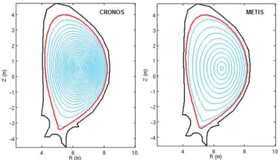
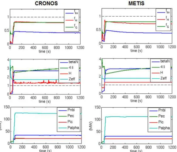
Snapshots of the equilibria in the flat-top phase are presented in Fig. 8, computed by CRONOS using the HELENA equilibrium code (i.e., full solution of the Grad-Shafranov equation) and by METIS (i.e., solution of equations for moments of the equilibrium, plus morphing function). For both simulations, the same LCFS has been assigned as an input. The shapes of the flux surfaces look very similar; some differences are seen in particular in the bottom area, which could be minimised by fine-tuning the parameters of the morphing function. The differences between the two equilibria can be analysed with further detail by plotting specific quantities related to the equilibrium, as shown in Fig. 9. Here again, the differences are minimal, and affecting in particular the region beyond ρ = 0.5. The time evolutions of several global quantities are compared in Fig. 10. Differences are found (e.g., the alpha power level is somewhat lower in the METIS simulation, li evolves in a slightly different way, etc.). Nevertheless, none of the important features of the scenario evolution, as found in the CRONOS simulation, is missed by METIS. The main reason for this is that METIS has the same type of non-linearities and interplays of the various quantities as CRONOS, only treated in a more approximated way.

Figure 8: ITER hybrid scenario: snapshots of computed equilibrium in the flat-top phase. CRONOS (left) and METIS (right) simulations.

24

Figure 9: ITER hybrid scenario: equilibrium related quantities in the flat-top phase, for CRONOS and METIS simulations. The various quantities are defined in connection with Eq. 1.

Spatial profiles are compared in Figs. 11-13. In both CRONOS and METIS simulations, pedestal density and temperature values are prescribed, and the density peaking has been adjusted in METIS. The resulting temperatures are rather similar (values and slopes in the gradient region, ratio Te/Ti), with the exception of the very central values, which are different by ~10%, as shown in Fig. 11. This difference is connected with the difference in the central alpha power, as shown in Fig. 12, since the evolutions of ion temperature and fusion power are non-linearly depending on each other. The other power deposition profiles shown in Fig. 12 are certainly different in shape (typically, the METIS source profiles are given analytically and therefore have smoother profiles), but none of these differences seems essential for the global accuracy of the simulation. A similar remark can be made for the current density profiles shown in Fig. 13. What is usually difficult to obtain in simulations of a hybrid scenario (as well as in experiments) is the careful balance of current sources (including the self-generated bootstrap), with an evolution in time leading to a stationary q profile that is flat in the central part and slightly higher than unity. As shown in Fig. 14, this is equally well obtained by both CRONOS and METIS codes, despite the wide differences of assumptions, approximations, resolution and computational time in the two simulations.

25

Figure 10: ITER hybrid scenario: time evolution of various quantities computed in CRONOS (left) and METIS (right) simulations. From top to bottom: bootstrap, non-inductive and Greenwald fractions; βN, à ∗ âã , H factor

and Zeff; NBI, ECRH, ICRH and alpha powers.

Figure 11: ITER hybrid scenario: computed density, electron and ion temperature profiles in the flat-top phase. CRONOS (left) and METIS (right) simulations.

26

Figure 12: ITER hybrid scenario: computed alpha, NBI, ECRH and ICRH power deposition profiles in the flat-top phase. CRONOS (left) and METIS (right) simulations.

Figure 13: ITER hybrid scenario: computed current density profile and contributions from NBI, ECCD and bootstrap, in the flat-top phase. CRONOS (left) and METIS (right) simulations.

27

Figure 14: ITER hybrid scenario: computed safety factor profile in the flat-top phase. CRONOS (solid) and METIS (dashed) simulations.

The application of METIS during the latest years has been rich and broad, covering several fundamental aspects in the field of integrated modelling. Some examples are summarized here.

Interpretive analysis of existing discharges in view of addressing some specific topic, for instance the study of the Experimental Advanced Superconducting Tokamak (EAST) upgraded operational space with higher input power [48], the calculation of particle sources in long steady-state Tore-Supra discharges [49], the assessment of the requirements of current-drive of steady-state regimes [50], or the analysis of the Lower Hybrid heating deposition [51].

One of the most important activities performed with METIS has been the assessment in terms of performance, calculation of density, temperature and toroidal velocity profiles or magnetic characteristics of tokamak devices which recently started operation, such as WEST [52, 53] or will do it in the future as JT-60SA [54], ITER [55, 56, 57] or DEMO [58, 59, 60, 61].

METIS has been used as current diffusion and equilibrium solver in a self-consistent integrated modelling chain involving the ray-tracing/Fokker Planck C3PO/LUKE in view of validating the prediction of Lower Hybrid current drive in Tore Supra experiments [62, 63, 64, 65, 66].

Among these applications, the fast integrated transport calculations provided by METIS are the most useful for the design of future scenarios and experiments. Indeed, scenario design is usually achieved by launching a large number of simulations varying the scenario parameters and following a “trial and error” approach. Being able to compute a full scenario faster than real time is therefore a key advantage for such a procedure. The scenario parameters may also include the parameters of control algorithms that may be used during the experiment. METIS can be integrated in a full tokamak Simulator, i.e. the integrated modelling of the control schemes (simulated outside of METIS) and the plasma response (provided by METIS) [67, 68, 69, 70]. For this purpose, METIS can act as a “one

28 time step” transport solver receiving control waveforms from the control schemes simulator. This application is usually implemented under Simulink®, a tool widely used to develop plasma control algorithms, in which METIS represents a single block providing the dynamic plasma response (and is easily integrated because it is written in Matlab®). An integrated design of tokamak scenario, including its control algorithms, can therefore be achieved and is greatly facilitated by the high speed of execution of METIS.

Because METIS is fast and features a large number of tunable options, it enables playing with a lot of physics parameters and model assumptions, allowing testing the sensitivity of the results to them. This allows in particular uncertainty quantification on the extrapolation to new devices. Models and assumptions have to be carefully chosen and justified depending of the application and goal of the simulation. As for any other kind of simulations, benchmarking a given set of models/assumptions on well documented experimental data increases confidence in extrapolation. In order to justify a posteriori the assumptions made, METIS results can be compared to more sophisticated models (transport, sources, …), run in stand-alone mode and using the plasma characteristics predicted by METIS as input in a few selected cases to be tractable. Being able to easily connect METIS output to other codes allows closing the gap between the simplified models used in METIS and more advanced and CPU-demanding models.

6

Conclusions

The METIS suite has been developed with the objective of achieving a fast integrated tokamak simulator with the simplest possible utilisation for physicists, flexibility in the type of simulations that can be carried out, and user-friendliness with a powerful and extensive graphical interface. The code employs innovative numerical schemes and simplified physical formulations, which capture the main physical features for scenario modelling, allowing fast and always convergent computation and realistic simulations. During the past 12 years, the METIS code has been validated against both experiments and simulation results. It is now a mature code, able to cope with a variety of integrated simulations for present and future tokamak devices, world widely used. METIS was originally a module of the CRONOS suite of codes and now it is also a standalone code which can be used alone or together with other codes inside the IMAS and EU-IM frameworks, within a Simulink workflow or inside Matlab or Python programs. This makes of METIS a versatile and adaptable code. METIS has been made available to many laboratories worldwide allowing as well modelling present and future experiments, as training students. METIS has been in the core of various collaborations and will continue in the future to open opportunities for collaboration, especially inside the IMAS framework. The main advantage of a common framework, such as IMAS, is to provide users from various laboratories with several modelling tools that can be handled and communicate in a common way. The integration of METIS into the IMAS framework and the recent adaptation of METIS GUI, including now dedicated tools for initialising WEST, JT-60SA and ITER/DEMO scenario simulations, allow METIS to be a key code for future studies, to generate first level modelling and to provide input data to other codes.

Acknowledgements

The work of J. Urban has been partially supported by Czech Science Foundation project GA16-24724S and MEYS projects 8D15001 and LM2015045

29

7

Appendix : Source modules

7.1

General description

A detailed description of the main source modules in METIS is provided in the following sections.

7.2

Bootstrap current and resistivity

The plasma neoclassical resistivity and bootstrap current profiles are computed using the Sauter model [10]. Optionally, the total bootstrap current can be normalized to the Hoang scaling law [71] – the shape of the bootstrap current density profile remaining as given by the Sauter model. These quantities are used in the current diffusion equation (1).

7.3

Neutral Beam Injection Heating and Current Drive

The Neutral Beam Injection (NBI) is described in METIS by a beam attenuation equation applied in a simplified geometry in order to calculate the fast ion source, then using an analytical solution of the Fokker-Planck equation for the fast ion distribution function.

The beam attenuation is computed for a few sub-beams spread around the tangential radius and the vertical tilt value to take into account the beam geometry. The vertical tilt is accounted for by projecting field values (i.e. density or temperature) on a tilted line. The beam intensity (ä) damping equation along the beam path is:

#å(U)

#U = − 5( )/5††( )ä( ) (25)

where is the coordinate along the beam path with the initial condition : ä( = 0) = äæ at the entrance of the plasma

and

/5††= /NŽ“², ¹²N, 5( ), r5( ), …5††( )• + /²L~“², ¹²N, 5( ), r5( ), ç²( ), ›œ%•( )• (26) where /_N is the stopping cross section [72] and /_²L is the increment of the stopping cross section due to fast ions [73]. The stopping cross section along the neutral path depends on the beam ion mass (“_²), the initial beam energy (¹_²N), the pitch angle at the point where the neutral particles are ionized (ç_²), the fast ion source (›_œ%•), the electron density ₅, the electron temperature r₅ and the plasma effective charge …_5††

The neutral beam path entrance point is taken in the equatorial mid-plane of the plasma (at … = …N) on the low field side and the radius of tangency is prescribed. The final value of Υ gives the fraction of the power that is not deposited in the plasma (shine-through).

From the power deposition (¸_²(1)), we subtract the first orbit losses that are computed with a simplified model: we suppose that most of the fast ions are trapped near the plasma edge and we compute the orbit width (è_,(1) ) as done in reference [74]. The fast ions created at a distance smaller than è_,(1) from the edge are lost. In order to simulate the broadening of the deposition profile due to orbit width we convolve the profile by a step function of width è_,(1).