Regional Policy Evaluation: Interactive Fixed Effects and Synthetic Controls

HAL Id: halshs-00849071

https://halshs.archives-ouvertes.fr/halshs-00849071

Preprint submitted on 30 Jul 2013

HAL is a multi-disciplinary open access

archive for the deposit and dissemination of sci-entific research documents, whether they are pub-lished or not. The documents may come from teaching and research institutions in France or

L’archive ouverte pluridisciplinaire HAL, est destinée au dépôt et à la diffusion de documents scientifiques de niveau recherche, publiés ou non, émanant des établissements d’enseignement et de recherche français ou étrangers, des laboratoires

Regional Policy Evaluation: Interactive Fixed Effects

and Synthetic Controls

Laurent Gobillon, Thierry Magnac

To cite this version:

Laurent Gobillon, Thierry Magnac. Regional Policy Evaluation: Interactive Fixed Effects and Syn-thetic Controls. 2013. �halshs-00849071�

WORKING PAPER N° 2013 – 24

Regional Policy Evaluation: Interactive Fixed

Effects and Synthetic Controls

Laurent Gobillon Thierry Magnac

JEL Codes: C21, C23, H53, J64, R11

Keywords: Policy evaluation, Linear factor models, Synthetic controls, Economic geography, Enterprise zones

P

-

S

E

48, BD JOURDAN – E.N.S. – 75014 PARIS TÉL. : 33(0) 1 43 13 63 00 – FAX : 33 (0) 1 43 13 63 10

Regional Policy Evaluation:

Interactive Fixed E¤ects and Synthetic Controls

Laurent Gobillon

INED and Paris School of Economics

Thierry Magnac

Toulouse School of Economics

First version: October 2012

This version July 4, 2013

Abstract

In this paper, we investigate the use of interactive e¤ect or linear factor models in regional policy evaluation. We contrast treatment e¤ect estimates obtained by Bai (2009)’s least squares method with the popular di¤erence in di¤erence estimates as well as with estimates obtained using synthetic control approaches as developed by Abadie and coauthors. We show that di¤erence in di¤erences are generically biased and we derive the support conditions that are required for the application of synthetic controls. We construct an extensive set of Monte Carlo experiments to compare the performance of these estimation methods in small samples. As an empirical illustration, we also apply them to the evaluation of the impact on local unemployment of an enterprise zone policy implemented in France in the 1990s.

Keywords: Policy evaluation, Linear factor models, Synthetic controls, Economic geography,

1

Introduction

It is becoming more and more common to evaluate the impact of regional policies using the tools of program evaluation derived from micro settings (see Blundell and Costa-Dias, 2009, or Imbens and Wooldridge, 2011 for surveys). In particular, enterprise and empowerment zone programs have received a renewed interest over recent years (see for instance, Busso, Gregory and Kline, 2012, Ham, Swenson, Imrohoroglu and Song, 2012, Gobillon, Magnac and Selod, 2012). Those programs consist in a variety of locally targeted subsidies aiming primarily at boosting local employment or the employment of residents. Their evaluations use panel data and methods akin to di¤erence in di¤erences that o¤er the simplest form of control of local unobserved characteristics that can be correlated with the treatment indicator. Nonetheless, speci…c issues arise when studying regional policies and the tools required to evaluate their impact or to perform a cost-bene…t analysis are di¤erent from the ones used in more usual micro settings.

The issue of spatial dependence between local units is important in the evaluation of regional policies. Outcomes are likely to be spatially correlated in addition to the more usual issue of serial correlation in panel data. There is thus a need for a better control of spatial dependence and more generally of cross-section dependence when evaluating regional policies. This is why more elaborate procedures than di¤erence in di¤erences are worth exploring and the use of factor or interactive e¤ect proved to be attractive and fruitful in micro studies (Carneiro, Hansen and Heckman, 2003). Interactive e¤ect models facilitate the control for cross-section dependence not only because of spatial correlations but also because areas can be close in economic dimensions which depart from purely geographic characteristics. This is the case for instance when two local units are a¤ected by the same sector-speci…c shocks because of sectoral specialisation even if these units are not neighbors.

Second, a key issue in policy evaluation is that treatment and outcomes might be correlated because of the presence of unobservables. It should also be acknowledged when using regional data that those unobservables di¤erencing local units might be multidimensional because the

1_{We are grateful to participants at seminars in Duke University, INED in Paris, Toulouse School of Economics,}

CREST in Paris, ISER at Essex and at the 2012 NARSC conference in Ottawa, for useful comments as well as to Sylvain Chabé-Ferret for fruitful discussions. We also thank DARES for …nancial support. The usual disclaimer applies.

underlying cycles of economic activities of local units are likely to be multiple. Interactive e¤ect models are aimed precisely at allowing the set of unobserved heterogeneity terms or factor loadings that are controled for to have a large dimension.

Moreover, the estimation of linear factor models in panels is relatively easy and asymptotic properties of estimates are now well known (Pesaran, 2006, Bai, 2009). Yet, there are only a few attempts in the literature to conduct regional policy evaluations using factor models (Kim and Oka, 2013) or using a kindred conditional pseudo-likelihood approach (Hsiao, Ching and Wan, 2012).

The contributions of this paper are threefold. We …rst provide results concerning the theoretical set-up. We clarify restrictions in linear factor models under which the average treatment on the treated parameter is identi…ed. We analytically derive the generic bias of the di¤erence-in-di¤erences estimator when the true data generating process has interactive e¤ects and the set of factor loadings is richer than the standard single-dimensional additive local e¤ect. Moreover, we derive from extant literature conditions on the number of treatment and control groups as well as on the number of periods under which factor model estimation delivers consistent estimates of the average treatment on the treated parameter.

Contrasting the estimation of linear factor models with the alternative method of synthetic controls is our second contribution. This alternative method was proposed by Abadie and Gardeaz-abal (2003) and its properties have been developed and vindicated in a model with factors (Abadie, Diamond and Hainmuller, 2010). Under the maintained assumption that the true model is a lin-ear factor model, we show that synthetic controls are equivalent to interactive e¤ect methods whenever matching variables (i.e. factor loadings and exogenous covariates) of all treated areas belong to the (convexi…ed) support of matching variables of control areas, a case that we call the interpolation case. This is not true any longer in the extrapolation case, that is, when matching variables of one treated area at least, do not belong to the support of matching variables in the control group.

Our third contribution is that we evaluate the relevance and analyze the properties of in-teractive e¤ect, synthetic control and di¤erence-in-di¤erences methods by Monte Carlo experi-ments. We use various strategies for interactive e¤ect estimation. First, a direct method estimates the counterfactual for treated units by linear factor methods in a restricted sample where

post-treatment observations for treated units are excluded. The second method estimates a linear factor model which includes a treatment dummy and uses the whole sample. Propensity score matching underlies the third method in which the score is conditioned by factor loading estimates obtained using the …rst method. Imposing common support constraints on factor loadings when estimating the counterfactual for treated units by linear factor methods provides the fourth method. We contrast these Monte Carlo estimation results with the ones we obtain by using synthetic controls and di¤erence in di¤erences.

We …nally provide the results of an empirical application of these methods to the evaluation of the impact of a French enterprise zone program on unemployment exits at the municipality level in the Paris region. This extends our results in Gobillon et al. (2012) in which we were using conditional di¤erence-in-di¤erences methods. We show that the estimated impact is robust to the presence of factors and therefore to cross-section dependence. We also look at other empirical issues of interest such as the issue of missing data about destination when exiting unemployment as well as entries into unemployment.

In the next Section, we brie‡y review the meager empirical literature that use factor models to evaluate regional policies. We construct in Section 3 the theoretical set-up and write restrictions leading to the identi…cation of the average treatment on the treated in linear factor models. Next, we derive the bias of di¤erence in di¤erences and describe the linear factor model estimation procedures. We derive the conditions that contrast their asymptotic properties with those of synthetic control methods. Monte Carlo experiments reported in Section 4 evaluate the small sample properties of the whole range of our estimation procedures. The empirical application and estimation results are presented in Section 5 and the last section concludes.

2

Review of the litterature

Kim and Oka (2013) estimate an interactive e¤ect model following Bai (2009) and provide a policy evaluation of the impact of changes in unilateral divorce state laws on divorce rates in the US. They …nd that interactive e¤ect estimates are smaller than di¤erence-in-di¤erences estimates. Furthermore, they estimate their model varying the number of factors and …nd that the model selection procedures proposed by Bai and Ng (2003) are not informative.

domestic product of two policies of convergence with mainland China that were implemented at the turn of this century. Their observations consist in various macroeconomic variables measured every quarter over ten years for Hong Kong and countries either in the region or economically associated with Hong-Kong. The authors argue that interactive models can be rewritten as models in which interactive e¤ects can be replaced by summaries of outcomes for other countries at the same dates using a conditioning argument. Indeed, common factors can be predicted using this information but this entails losses of information since information at current period only is used to construct these predictions.

Interestingly, Ahn, Lee and Schmidt (2013) analyze an interactive e¤ect model and their method potentially provides e¢ ciency improvements over the procedure of Hsiao, Ching and Wan (2012). The authors show that the conditional likelihood function (or pseudo-likelihood function associated to the normal distribution), conditional on a number of period outcomes equal to the number of factors can be written as a function that does not depend on individual factor loadings. Assuming out any remaining spatial correlation, they show that conditional likelihood estimates are consistent for …xed T .

Overall, in a large N and T environment, the most prominent estimation methods were pro-posed by Pesaran (2006) who uses regressions augmented with cross section averages of covariates and outcomes, and by Bai (2009) who uses principal component methods. Westerlund and Urbain (2011) review quite extensively di¤erences between these methods.

3

Theoretical Set-Up

Consider a sample composed of i = 1; :::; N local units observed at dates t = 1; :::; T . A simple

binary treatment, Di 2 f0; 1g, is implemented at date TD < T so that for t > TD > 1, the units

i = 1; :::; N1 are treated (Di = 1). Units i = N1 + 1; :::; N are never treated (Di = 0). For each

unit, we observe outcomes, yit, which might depend on the treatment and the average e¤ect of the

treatment on the treated is our parameter of interest. In Rubin’s notations, we denote by yit(d)

the outcome of an individual i at date t if in treatment status d (where d = 1 in case of treatment, and d = 0 in the absence of treatment). This hypothetical status should be distinguished from

The average e¤ect of the treatment on the treated can be written when t TD:

E (yit(1) yit(0)jDi = 1 ) = E (yit(1)jDi = 1 ) E (yit(0)jDi = 1 ) (1)

A natural estimator of the …rst right-hand side term is its empirical counterpart since the

outcome in case of treatment is observed for the treated at periods t> TD. In contrast, the second

right-hand side term is a counterfactual term since the outcome in the absence of treatment is not

observed for the treated at periods t > TD. The principle of evaluation methods relies on using

additional restrictions to construct a consistent empirical counterpart to the second right-hand side term (e.g. Heckman and Vytlacil, 2007). For instance, it is well known that di¤erence-in-di¤erences methods are justi…ed by an equal trend assumption:

E(yit(0) yi;TD 1(0)j Di = 1) = E(yit(0) yi;TD 1(0)j Di = 0) for t TD: (2)

under which the counterfactual can be written as:

E (yit(0)jDi = 1 ) = E(yit(0) yi;TD 1(0) j Di = 0) + E(yi;TD 1(0)j Di = 1) for t TD;

in which all terms on the right-hand side are directly estimable from the data.

The object of this section is to generalize the usual set-up in which di¤erence in di¤erences provide a consistent estimate of the e¤ect of the treatment on the treated (TT) to a set-up allowing for higher-dimensional unobserved heterogeneity terms. Local units treated by regional policies could indeed be a¤ected by various common shocks describing business cycles related for instance to di¤erent economic sectors. Associated factor loadings would describe the heterogeneity of exposition of local units to these common shocks. A single dimensional additive local e¤ect as in the set up underlying di¤erence-in-di¤erences estimation is unlikely to describe this rich economic environment. Furthermore, we know that di¤erence in di¤erences can dramatically fail when heterogeneity is richer than what is modelled (Heckman, Ichimura and Todd, 1997).

In this paper, we restrict our attention to linear models because the number of units is rather small although extensions to non-linear settings could follow the line of Abadie and Imbens (2011) at the price of losing the simplicity of linear factor models. The route taken by Conley and Taber (2011) to deal with small sample issues might also be worth extending to our setting. More speci…cally, linearity makes one wary of issues of interpolation and extrapolation that we shall

highlight in the general framework of linear factor models as well as in the approach of synthetic controls proposed in the seminal paper by Abadie and Gardeazabal (2003).

We present in the …rst sub-section the maintained speci…cation of a linear factor model and we discuss identifying assumptions. Next, we show that the conventional di¤erence-in-di¤erences estimate is generically biased. We propose an estimation method by linear factor models including a treatment dummy and derive a rank condition for the identi…cation of the average treatment on the treated. We also propose a direct estimation method by constructing the counterfactual term in equation (1) using the samples of control and treated units albeit the latter before treatment only (see Heckman and Robb, 1985 or Athey and Imbens, 2006). Finally, we describe the approach of synthetic controls and analyze its properties when the true model has interactive e¤ects.

3.1

Interactive linear e¤ects and restrictions on conditional means

In the conventional case of di¤erence in di¤erences (DID) in which covariates are controlled for (see for instance Blundell and Costa-Dias, 2009), the outcome in the absence of treatment is speci…ed as a linear function:

yit(0) = xit + ~i+ et+ "it (3)

in which xitis a 1 K vector of individual covariates, and ~i and etare individual and time e¤ects.

A limit to this speci…cation is that individuals are all a¤ected in the same way by the time e¤ects. To allow for interactions and make the speci…cation richer, we specify the outcome in the absence of treatment as a function of the interaction between factors varying over time and heterogenous individual terms called factor loadings as:

yit(0) = xit + ft0 i+ "it (4)

i is a L 1vector of individual e¤ects or factor loadings, and ft is a L 1vector of time e¤ects

or factors. Note that this speci…cation embeds the usual additive model by letting i = ~i; 1

0

and ft= 1; et

0

as, in that case, f0

t i = ~i+ et.

The true process generating the data is supposed to be given by equation (4) and is completed by the description of the outcome in case of treatment:

which, in contrast to the linear speci…cation above, is not restrictive.

There are a few usual assumptions that complete the description of the maintained true model. First, we shall assume that we know the number of factors in the true model described by equation (4). Various tests regarding the number of factors might be useful to implement (Bai and Ng, 2002, Moon and Weidner, 2010b) but these are fragile (Onatski, Moreira and Hallin, 2011). Moreover, we adopt the assumption that factors are su¢ ciently strong so that the consistency condition for the number of factors and consequently for factors and factor loadings is satis…ed (for alternative views see Onatski, 2012 or Pesaran and Tosetti, 2011). This condition re‡ects the fact that factor

loadings can be separated from the idiosyncratic random terms at the limit.2

Moreover, we do not specify the dynamics of factors in the spirit of Doz, Giannone and Reichlin (2011). Their speci…cation imposes more restrictions on the estimation although inference is more di¢ cult to develop. This is why we stick to the limited information framework which does not impose conditions on the dynamics of factors although it could be done in the way explained by Hsiao, Ching and Wan (2012). Furthermore, the only available explanatory variables are not varying over time in our empirical application. This corresponds to the low rank regressor assumption as de…ned by Moon and Weidner (2010a) and under which identifying assumptions are of a particular form. At this stage however we prefer to stick to the more general format.

A …nal comment is worth making. In treatment evaluation, lagged endogenous variables are at times included as matching covariates in order to control for possible ex-ante di¤erences. In spirit, this is very close to a model with interactive e¤ets because it is well known that a simple linear dynamic panel data model like:

yit = yit 1+ i+ uit

can be rewritten as a static model:

yit= tyi0+ 1 t i

1 + it

in which it is an AR(1) process. Factors are t and 1 t; and factor loadings are yi0 and ₁ i .

This argument could be generalized to more sophisticated dynamic linear models.

3.1.1 Restrictions on conditional means

To complete the description of the true data generating process, we now present and comment the main restrictions on random terms. To keep notations simple and conform with the usual panel

data set up, we generally consider that factors ft are …xed while factor loadings i are supposed

to be correlated random e¤ects.

We …rst assume that idiosyncratic terms "it are "orthogonal" to factor loadings and that

explanatory variables are strictly exogenous:3

"it ? ( i; xi)

in which x0

i = (x0i1; :::x0iT)0 is a [T; K] matrix. This would be without loss of generality when

orthogonality is de…ned as the absence of correlation as in Bai (2009). Because of the next assumption we will adopt, we prefer to interpret orthogonality as mean independence and the translation of the above assumption is therefore that:

Assumption A1: E("itj i; xi) = 0:

Second, we extend the usual assumption made in di¤erence-in-di¤erences estimation by assuming that the conditioning set now includes unobserved factor loadings:

yit(0) ? Di j (xi; i), "it ? Di j (xi; i)

and we write this condition as a mean independence restriction:

Assumption A2: E("itj Di; i; xi) = E("it j i; xi):

Note that we do not suppose that ( i; xi)and Di are uncorrelated and selection into treatment

can freely depend on observed and unobserved heterogeneity terms.

Finally, de…ne the average treatment e¤ect over the periods after treatment as: i = 1 T TD+ 1 T X t=TD it

so that our main parameter of interest is the average treatment on the treated over the periods

after treatment de…ned as:4

3_{The extension to the case with weakly exogeneous regressors would follow Moon and Weidner (2010a) for}

instance.

4_{In the case T ! 1, those de…nitions should be interpreted as limits. Note also that it is generally easy to}

design estimates for time-speci…c treatment parameters such as E( itj Di = 1) by restricting the post-treatment

De…nition ATT: = E( i j Di = 1) = 1 T TD+ 1 T X t=TD E( itj Di = 1):

Assumptions A1 and A2 are the main restrictions in our set-up and De…nition ATT de…nes our parameter of interest.

3.2

The generic bias of di¤erence-in-di¤erences estimates

If the true data generating process comprises interactive e¤ects, we now show that the di¤erence-in-di¤erences estimator is generically biased although we exhibit two interesting speci…c cases in which the bias is equal to zero. For simplicity, we omit covariates or, since covariates are assumed to be strictly exogenous, implicitly condition on them in this subsection. We also assume for

simplicity that the probability measure of factor loadings in the treated population, dG( i j Di =

1); and in the control population dG( i j Di = 0), are dominated by the Lebesgue measure so

that both distributions are absolutely continuous.

We shall show that the condition which is implied by Assumption A2:5

E(yit(0) yi;TD 1(0) j Di = 1; i) = E(yit(0) yi;TD 1(0) j Di = 0; i) for t> TD (6)

does not imply equation (2) under which the di¤erence-in-di¤erences estimator is consistent. Indeed:

E(yit(0) yi;TD 1(0) j Di = 1) = E [E(yit(0) yi;TD 1(0) j Di = 1; i)] ;

=R E(yit(0) yi;TD 1(0) j Di = 1; i)dG( i j Di = 1):

Replacing the integrand using equation (6) yields:

E(yit(0) yi;TD 1(0)j Di = 1) =

Z

E(yit(0) yi;TD 1(0)j Di = 0; i)dG( i j Di = 1): (7)

Two special cases are worth noting. Firstly, the integrand in the previous expression does not

depend on i in the restricted case in which there is a single factor ft = 1 and a single individual

e¤ect associated with this factor. In this case, equation (7) can be written as:

E(yit(0) yi;TD 1(0)j Di = 1) = E(yit(0) yi;TD 1(0)j Di = 0)

R

dG( i j Di = 1)

= E(yit(0) yi;TD 1(0)j Di = 0);

which yields equation (2) describing equality of trends.

Alternatively, (perfectly) controled experiments also enables identi…cation through di¤erence

in di¤erences in spite of using the alternative argument that dG( i j Di = 1) = dG( i j Di = 0):

The same equation (2) holds and the treatment parameter is consistently estimable by di¤erence in di¤erences.

This implication is not true in general and we can distinguish two cases. If the conditional

distribution of i in the treated population is dominated by the corresponding measure in the

control population i.e.:

8 i such that dG( i j Di = 0) = 0we have dG( i j Di = 1) = 0; (8)

the support of the treated units is included in the support of the non treated units. We shall describe from now on cases in which support condition (8) holds as an instance of interpolation and if such a condition is not satis…ed, as an instance of extrapolation.

In the interpolation case, let:

r( i) =

dG( i j Di = 1)

dG( i j Di = 0)

<₁

which is well de…ned because of the support condition (8) and because distributions are absolutely continuous. Write equation (7) as:

E(yit(0) yi;TD 1(0) j Di = 1) =

Z

E(yit(0) yi;TD 1(0) j Di = 0; i)r( i)dG( i j Di = 0) (9)

which in turn implies that:

E(yit(0) yi;TD 1(0)j Di = 1) = E(yit(0) yi;TD 1(0)j Di = 0)

+Cov (yit(0) yi;TD 1(0); r( i)j Di = 0)

The second term in the right hand side can be interpreted as the di¤erential trend in outcomes which is due to the time varying e¤ects of factors interacted with unobserved factor loadings. If there is indeed a factor loading associated to a time-varying factor, the second term is not equal to zero except under special circumstances as seen above. In the interpolation case, the second term describes the bias in DID estimates.

In the alternative case of extrapolation, the bias term is derived in a similar way although its interpretation is less clear since it mixes issues of non inclusive supports with the time varying e¤ect of factors.

3.3

Interactive E¤ect Estimation in the Whole Sample

We now explore interactive e¤ect methods and exhibit conditions under which these methods allow the identi…cation of the average treatment on the treated parameter.

The observed outcome veri…es:

yit = yit(0)1fDit= 0g+yit(1)1fDit= 1g

and using equations (4) and (5), it can be written as:

yit = itItDi+ xit + ft0 i+ "it (10)

in which Di is the treatment indicator, and It= 1ft TDg is an indicator of treated periods. We

maintain Assumptions A1 and A2 that allow the correlation between Di and i to be unrestricted

so that selection into treatment can depend on factor loadings. Similarly, the correlation between

It and ft is unrestricted so that the implementation of the treatment can be correlated with

economic cycles which are described here by factors. We shall rewrite equation (10) as:

yit= ItDi+ xit + ft0 i+ "it+ ( it )ItDi (11)

in which is the average treatment on the treated parameter as in De…nition ATT.

We now exhibit conditions under which can be estimated using interactive e¤ect procedures

as proposed by Bai (2009). We start with the case = 0which requires a weak rank condition and

then extend it to the general case with covariates which requires a stronger additional assumption albeit easy to interpret.

3.3.1 Average Treatment E¤ect on the Treated in the Absence of Covariates

We shall prove that the parameter of interest is identi…ed under the two conditions that It is

not equal to a linear combination of factors ft and that the probability of treatment is positive.

We continue considering that T is …xed as well as factors ft and treatment It and we analyze

identi…cation as if factors ft were known. This argument extends to the case in which T tends to

in…nity by taking limits.

Stack individual observations in individual vectors of dimension [T; 1] :

in which yi = (yi1; :; yiT)0; I[1:T ] = (I1; :; IT)0; F = (f1; :; fT); "i = ("i1; :; "iT)0 and

i = diag ( i1 ; :::; iT ) is a matrix of dimension [T; T ]. Set MF = I F0(F F0) 1F and

multiply the previous equation to obtain:

MFyi = DiMFI[1:T ]+ MF"i+ MF iI[1:T ]Di: (13)

A necessary condition of identi…cation of using the latter equation stacked over the di¤erent

individual units is that:

I_{[1:T ]}0 MFI[1:T ] > 0 and E(Di) > 0; (14)

which means that I[1:T ] is not equal to a linear combination of factors and that the probability

of being treated is positive. This is related to the rank condition underlying the identi…cation of parameters as in Proposition 3 in Bai (2009, p.1259). Furthermore, this condition is also necessary

in equation (12) because the correlation between i and Di is unrestricted.

This condition is also su¢ cient since E(Di)I[1:T ]0 MFI[1:T ] is invertible and because we now show

that:

= (E(DiI[1:T ]0 MFI[1:T ])) 1E(DiI[1:T ]0 MFyi) = (E(Di)I[1:T ]0 MFI[1:T ]) 1E(DiI[1:T ]0 MFyi): (15)

Indeed, the correlation between the two right-hand side terms of equation (13), the regressor DiMFI[1:T ] and the error term MF"i + MF( i )I[1:T ]Di; is equal to zero. There are two terms in this correlation that we analyze in turn.

The …rst term is equal to 0 by construction (Assumption A2):

E(I_{[1:T ]}0 MFDiMF"i) = E(I[1:T ]0 MFDiMFE("i j Di)) = 0 (16)

since Di is a scalar random variable and variables in the time dimension are supposed to be …xed.

The second term of the correlation above is more interesting and can be written as:

E(I_{[1:T ]}0 MFDiMF iI[1:T ]Di) = E(I[1:T ]0 MFDiMFE( iI[1:T ]j Di)Di); (17)

which is equal to zero by construction of i since by De…nition ATT:

E( iI[1:T ] j Di = 1) = E( T X t=TD ( it )j Di = 1) = 0: Multiplying (13) by I0

[1:T ]MFDi and taking the expectation gives (15). This ends the proof that

3.3.2 The Case with Covariates

In the general case with covariates, we can write equation (11) as: yi = DiI[1:T ]+ xi + F0 i+ "i+ iI[1:T ]Di

Multiplying this equation by MF, we obtain:

MFyi = DiMFI[1:T ]+ MFxi + MF"i+ MF iI[1:T ]Di: (18)

Denote the linear prediction of Di as a function of xi as:

Di = vec(xi)0 + Dix;

and rewrite equation (18) as:

MFyi = DixMFI[1:T ]+ MF~"i + MF iI[1:T ]Di; (19)

in which ~"i = "i+ xi + :vec(xi)0 I[1:T ]. Because xi and vec(xi) are uncorrelated with Dix; the

same non correlation condition as in equation (16) is valid since we have from Assumptions A1 and

A2 that E ("ijDi; xi) = 0. Thus, the second condition derived from equation (17) that remains

to be checked refers to the equality to zero of:

E( iI[1:T ]DiDix) = E( iI[1:T ]DiDi) E(( iI[1:T ]Divec(xi)0 ) = E( iI[1:T ]Divec(xi)0 ); because of the argument employed after equation (17) that uses De…nition ATT. This correlation is equal to zero under the su¢ cient condition given by:

E( itj Di = 1; xi) = E( itj Di = 1);

since it implies that:

E( iI[1:T ] j Di = 1; xi) = E( iI[1:T ] j Di = 1) = 0;

by De…nition ATT as above. This condition is stronger than necessary as it would be su¢ cient

to condition on the scalar variable vec(xi) .6 Note also that the linear interactive model could be

6_{In this case, developments following Wooldridge (2005) might be appropriate but we do not follow up this}

generalized by conditioning on covariates or interacting covariates with the treatment indicator and this would substantially weaken this condition as in the static evaluation case (Heckman and Vytlacil, 2007).

Consistency and other asymptotic properties of this method can be derived from Bai (2003)

when N _{! 1 and T ! 1. Note also that condition (14) also implies that N}1 tends to 1 when

N _{! 1. Estimation could also proceed with the estimation method proposed by Ahn, Lee and}

Schmidt (2013) and thence dispenses with the assumption that T ! 1.

3.4

Direct Estimation of the Counterfactual

Assumptions A1 and A2 imply that a direct estimation strategy for the treatment on the treated e¤ects can also be adopted. Estimate …rst the interactive e¤ect model (4) using the sample com-posed of non treated observations over the whole period and of treated observations before the

date of the treatment t < TD. Orthogonality assumption A2 makes sure that excluding

obser-vations i 2 f1; :; N1g and t TD does not generate selection. Second, orthogonality assumption

A1 renders conditions stated by Bai (2009) valid and the derived asymptotic properties of linear factor estimates hold under identifying restrictions as stated in Moon and Weidner (2010b).

Various asymptotics can then be considered:

If N and T tend to 1, then , ftand i for the non treated are consistently estimated (Bai,

2009).

If additionally the number of periods before treatment TD tends to 1, then i for the treated

units are consistently estimated.

As for the counterfactual term to be estimated in equation (1), we have for t> TD:

E (yit(0)jDi = 1 ) = E (xit + 0iftjDi = 1 ) (20)

To estimate this quantity, we replace parameters i, i = 1; :::; N1, and ft when t> TD by their

consistently estimated values in the right-hand side expression (computed as detailed in Appendix A.2), and take the empirical counterpart of the expectation. Namely, the treatment on the treated at a given period is derived by using equation (1) and can be written as:

and its estimate is obtained by replacing unknown quantities by their empirical counterparts. The average treatment on the treated e¤ect is then obtained by exploiting De…nition ATT and

averaging equation (21) over the periods after treatment.7

An additional word of caution about identi…cation is necessary since the rank condition (14) developed in the previous section also applies although it is not as simple to derive. This is summarized in the next proposition:

Proposition 1 Suppose that rank condition (14) does not apply and that the treatment indicator

IT is a linear function of factors:

IT = F0

in which is a [L; 1] vector and F is the matrix of factors as de…ned above. Then for any value of

the treatment e¤ect ; there exists an observationally equivalent factor model in which the value

of the treatment e¤ect is equal to zero.

Proof. Let be any value and write equation (12) as

yi = ITDi+ F0 i+ ~"i

in which ~"i includes any idiosyncratic variation of the treatment e¤ect across individuals and

periods. By replacing IT = F0 ; we get:

yi = F0 Di+ F0 i+ ~"i;

= F0( Di+ i) + ~"i;

which provides the alternative factor representation in which the value of the treatment e¤ect is equal to zero.

This result implies that condition (14) applies to the estimation method derived in this section as well as to any other estimation method analyzed below.

3.5

A single-dimensional factor model

It is well known since Rubin and Rosenbaum (1983) that conditions A1 and A2 imply the condition:

E("it j Di = 1; p(xi; i)) = 0

in which the distinction between observed variables xiand unobserved variables idoes not matter.

Let i = p(xi; i) denote the propensity score.

The condition above suggests the following strategy:

1. Estimate factors and factor loadings using the sample of controls and the subsample of treated observations before treatment as detailed in Subsection 3.4.

2. Regress Di on xi and ^i and construct the predictor of the score ^i:

3. Match on the propensity score à la Heckman, Ichimura and Todd (1998), or, under some

conditions, use a single factor model associated to ^_i.

3.6

Synthetic controls

The technique of synthetic controls proposed by Abadie and Gardeazabal (2003) and further explored by Abadie, Diamond and Hainmueller (2010, ADH thereafter) proceeds di¤erently. It focuses on the case in which the treatment group is composed of a single unit and uses a speci…c matching procedure of this treated unit to the control units whereby a so-called synthetic control is constructed. We shall proceed in the same way although as we have potentially more treated units, we shall repeat the procedure for each of them and then aggregate the result over various

synthetic controls to yield the average treatment on the treated.8

3.6.1 Presentation

We follow the presentation by ADH (2010). An estimator of yit(0) for a single treated unit i 2

f1; :; N1g after treatment t TD is the outcome of a synthetic control “similar” to the treated

unit which is constructed as a weighted average of non-treated units. We impose similarity of

characteristics xit between treated units and synthetic controls, by weighting characteristics xjt of

8_{An alternative would be to aggregate the treated units into a single unit …rst. By analogy with what is done}

in non-parametric matching, this procedure seems more restrictive because constructing a single synthetic control leads to less precise estimates than when constructing various synthetic controls. Nonetheless, support conditions for the validity of the synthetic control method that we …nd might justify such an approach because support requirements are weaker in the "aggregate" case.

control units, j 2 fN1+ 1; :; Ng in such a way that N

X j=N1+1

!(i)_j xjt = xit for t = 1; :; T (22)

where !(i)_j is the weight of unit j in the synthetic control (such that !(i)_j > 0 and

N P j=N1+1

!(i)_j = 1).

Similarity between pretreatment outcomes is also imposed in ADH (2010): N X j=N1+1 !(i)_j y_j(k)= y(k)_i (23) where y_j(k)= TDP1 t=1

ktyjt is a weighted average of pretreatment outcomes in which k = (k1; :; kTD 1)

are weights di¤ering across periods (y(k)_i for the treated unit is de…ned similarly). A set of such

pre-treatment outcome summaries can be generated using various vectors of weights, k: Nevertheless,

the most general setting is when we consider all pretreatment outcomes, yjt; for t = 1; :::; TD 1.

Indeed, taking linear combinations of pretreatment outcomes or considering the original ones is

equivalent in this general formulation and we dispense with the construction of y_j(k) and y_i(k).

The average treatment on the treated for unit i is estimated as:

^i = 1 T TD+ 1 X t TD " yit N X j=N1+1 !(i)_j yjt # : (24)

In practice, one needs to determine the weights that allow us to construct the synthetic control. Weights should ensure that the synthetic control is as close as possible to the treated unit i and

thus that conditions (22) and (23) are veri…ed. Denote zj = (yj1; :; yj;TD 1; xj1; :; xjT)0 (resp. zi)

the list of variables over which the synthetic control is constructed (i.e. pretreatment outcomes and exogenous variables). Weights are computed using the following minimization program:

M in !(i)_j !(i)_j >0; N P j=N1+1 !(i)_j =1 N X j=N1+1 !(i)_j zj zi !0 M N X j=N1+1 !(i)_j zj zi ! (25)

in which M is a weighting matrix.9 Note that the resulting weight !(i) is a fonction of the data

(zi; zN1+1; :; zN):

9_{M can be chosen in various ways (see Abadie et al, 2010, for some guidance). In our case we set M to the}

3.6.2 Synthetic controls and interactive e¤ects

We now describe this procedure in an interactive e¤ect model as …rst suggested by AHD (2010). Nonetheless, we show that the absence of bias implies constraints on the supports of the factor loadings and of exogenous variables and is related to the developments in Section 3.2 above.

To proceed, we need to introduce additional notations. Our linear factor model can be written at each time period as:

Yt(0) = 0Xt0+ ft0 U + "t for the untreated,

yit(0) = 0x0it+ ft0 i+ "it for each treated individual

(26)

where U = ( N1+1; :::; N) is (L; N N1) and ft is a L column vector. Similarly, Yt(0) and "t

are (N N1) row vectors and Xt is a (N N1; K) matrix.

As weights !(i) _{= !}(i)

N1+1; :::; !

(i)

N are obtained by equation (25), we have:

8 < :

yit(0) = Yt(0) !(i)+ it for t < TD,

x0

it= Xt0!(i)+ itX for t = 1; :::; T

(27)

Note that the construction of the synthetic control by equation (27) is allowed to be imperfectly

achieved and the discrepancy is captured by the terms _it and _itX. We thus acknowledge that

characteristics of the treated unit, zi = (yi1; :; yi;TD 1; xi1; :; xiT)0, might not belong to the cone

CU generated by the characteristics of control units. First, there are small sample issues when

the number of pre-treatment periods, TD 1, and of covariates, KT , is larger than the number

of untreated units, N N1. In other words, cone CU lies in a space whose dimension is lower

than the number of vector components, TD 1 + KT . Second and more importantly, even if

TD 1 + KT < N N1, vector zi might not belong to this cone because supports of characteristics

for treated and control units di¤er. Terms _it and _itX capture this discrepancy.

We now analyze what consequences this construction has on the estimation of the treatment e¤ect. The estimated treatment e¤ect given by equation (24) is a function of

yit

N X j=N1+1

!(i)_j yjt = yit(1) Yt(0) !(i) = it+ yit(0) Yt(0) !(i)

= it+ it;

in which we have extended de…nition (27) to all t TD. The absence of bias of the LHS estimate

primitives, we need to replace dependent variables by their values in the model described by (26). This delivers:

it = yit(0) Yt(0) !(i) = 0x0it+ ft0 i+ "it ( 0Xt0 + ft0 U + "t)!(i);

= 0(x0_it X_t0!(i)) + f_t0( i U!(i)) + "it "t!(i):

Considering that and ft are …xed and taking expectations yields:

E( _it) = 0E(x0_it X_t0!(i)) + f_t0E( i U!(i)) + E("it "t!(i));

' 0E(x0_it X_t0!(i)) + f_t0E( i U!(i));

in which we have used the result derived by ADH (2010) that E("it "t!(i))tends to 0 when the

number of pretreatment periods TD tends to 1.10 This expression should be true for any value of

and ft and the absence of bias thus implies that:

E(x0_it X_t0!(i)) = 0 and E( i U!(i)) = 0: (28)

A su¢ cient condition is established in Appendix B:

Lemma 2 If the support of exogenous variables and factor loadings of the treated units is a subset

of the support of exogenous variables and factor loadings of the non treated units and this latter

set is convex and bounded then condition (28) is satis…ed at the limit when N N1 ! 1.

We call this case the interpolation case and this relates to the familiar support condition in the treatment e¤ect literature and to the domination relationship between probability measures in the treated and control groups seen in equation (8) above.

If this property is not true, the synthetic control method is based on extrapolation since it

consists in projecting i and xit onto a cone to which they do not belong and this generates a

bias. For instance, to compute the distance between i and the convex cone conv ( U), we could

use the support function (see Rockafellar, 1970) and show that:

d ( i; conv ( U)) = inf

q2RL _j2fNmax_{1+1;:::;N g}(q

0

j) q0 i

in which j is the j-th column of U. Statistical methods to deal with inference in this setting

could be derived from recent work by Chernozhukov, Lee and Rosen (2013) but this is out of the scope of this paper.

10_{The main di¢ culty there is to take into account that ! is a random function of z}

3.6.3 Constraints on linear factor models

The conditions of interpolation implies constraints on the linear factor model that can be imposed when estimating the parameters involved in (20). They are developed in Appendix A.2.

4

Monte Carlo experiments

4.1

The set-up

The data generating process is supposed to be given by a linear factor model:

yit = iItDi+ ft0 i+ "it

in which the treatment e¤ect, i, is homogeneous or heterogenous across local units (but not

time for simplicity) and the number of factors L is variable. Residuals "it are supposed to be

independently and identically distributed. We always include additive individual and time e¤ects,

i.e. i = ( i1; 1; i2; :::)0 and ft = (1; ft1; ft2:::)0 as most economic applications would require. We

did not include any other explanatory variables than the treatment variable itself.

The data generating process is constructed around a baseline experiment and several alter-native experiments departing from the baseline in di¤erent dimensions such as the distribution of residuals, the number of local units and periods, the correlation of treatment assignment and factor loadings, the structure of factors, the support of factor loadings and the heterogeneity of the

treatment e¤ect, i. Experiments are described in detail below. The Monte Carlo aspect of each

experiment is given by drawing new values of f"itgi=1;:;N;t=1;:;T only and the number of replications

is set to 1000.

In the baseline, individual and period shocks "it are drawn in a zero-mean and unit-variance

normal distribution and we experiment an alternative in which shocks are drawn in a uniform

distribution [ p3;p3], the bounds being chosen to get a zero mean and a unit variance.

The numbers of treated units, N1(resp. total, N ) and the numbers of periods before treatment,

TD, (resp. total, T ) as well as the number of factors L are …xed at relatively small values in line

with our empirical application developed in the next section and more generally with data used

in the evaluation of regional policies. In the baseline experiment, we …x (N1; N ) = (13; 143),

(25; 275), (TD; T ) = (4; 10)and L varying in the set f2; 4; 5; 6g.

The values of factors ft and factor loadings, i are drawn once and for all in each experiment.

Factors, ft; for t = 1; :; T; are drawn in a uniform distribution on [0; 1] (except the …rst factor

which is constrained to be equal to 1). Alternatively, we also experiment in having the second

factor in ft given by a: sin(180:t=T ) with a > 0 large enough.

The support of factor loadings, i, is the same for treated units as for untreated units in

our baseline experiment. They are drawn in a uniform distribution on [0; 1] (except the second factor loading which is constrained to be equal to 1). In an alternative experiment, we construct overlapping supports for treated and untreated units. This is achieved by shifting the support of factor loadings of treated units by :5 or equivalently by adding :5 to draws. In another experiment, supports of treated and untreated units are disjoint by shifting the support of treated units by 1. Because the original support is [0; 1], this means that the intersection of the supports of treated and non-treated units is now reduced to a point. Note that adding :5 (resp. 1) to draws of treated

units creates a correlation between factor loadings and the treatment dummy Di equal to :446

(resp. :706).

The treatment e¤ect is constant, i = , in our baseline experiment while in alternative

experiments, the treatment e¤ect is correlated with the second individual factor, the …rst factor

loading, i1 being the standard linear …xed e¤ect. The heterogenous treatment parameter is thus

written as i = + r: i2 _N1₁

XN1

i=1 i2 . This speci…c form is retained to make sure that the

average treatment on the treated is equal to by construction as we have: _N1

1

XN1

i=1 i = .

In practice, we …x = :3 which is a value close to ten times the one obtained in our empirical

application, and r = 1.

We evaluate six estimation methods:

1. A direct approach using pretreatment period observations for control and treated units and

post-treatment periods for the non treated only to estimate factors ftand i in the equation:

yit(0) = ft0 i+ "it (29)

as in Section 3.4. The estimation procedure follows Bai’s method and is based on an EM

from equation (21) replacing the right-hand side quantities by their empirical counterparts. This estimator is labelled “Interactive e¤ects, counterfactual”.

2. An approach whereby we estimate parameter applying Bai’s method to the linear model

in which a treatment dummy is the only regressor:

Yit= ItDi+ ft0 i+ "it

as in Section 3.3. The resulting estimator is labelled “Interactive e¤ects, treatment dummy”. 3. A matching approach (Subsection 3.5) by which equation (29) is …rst estimated as in the …rst

estimation method. This yields estimates of i from which a propensity score discriminating

treated and untreated units is computed. We use a logit speci…cation for the score and construct the counterfactual outcome in the treated group in the absence of treatment at

periods t> TD using the kernel method proposed by Heckman, Ichimura and Todd (1998).

If we denote the score predicted by the logit model by ^i, the counterfactual of the outcome

for a given treated local unit i at a given post-treatment period is constructed as: b E (yit(0)jDi = 1 ) = XN j=N1+1 Kh ^i ^j yjt .XN j=N1+1 Kh ^i ^j for t> TD

where Kh( ) is a normal kernel whose bandwidth is chosen using a rule of thumb

(Sil-verman, 1986). An estimator of the average treatment on the treated is the average of

yit E (yb it(0)jDi = 1 ) over the population of treated local units for dates t > TD. The

resulting estimator is labelled “Interactive e¤ects, matching”.

4. An approach similar to “Interactive e¤ects, counterfactual” in which we impose the

con-straint i = U!(i) for any unit i when estimating (29). U is the L (N N1) matrix

comprising untreated factor loadings and !(i) _{are weights obtained in the synthetic control}

method. The estimation method is detailed in Appendix A.2 and the estimator of is

re-covered from (21) replacing right-hand side quantities by their empirical counterpart. This estimator is labelled “Interactive e¤ects, constrained”.

5. The synthetic control approach (Subsection 3.6) whereby the average treatment on the treated is obtained by averaging equation (24) over the population of treated units. The resulting estimator is labelled “Synthetic controls”.

6. A standard di¤erence-in-di¤erences approach whereby we compute the FGLS estimator tak-ing into account the covariance matrix of residuals (written in …rst di¤erence). Recent research presented in Brewer, Crossley and Joyce (2013) suggests that this is the appropri-ate procedure if assumptions underlying di¤erence in di¤erences are satis…ed. The resulting estimator is labelled “Di¤-in-di¤s”.

In our simulations, the number of iterations for Bai’s method involved in methods (1) to (4) is …xed to 20, and the number of iterations for the EM algorithm involved in method (1) and (4) is …xed to 1. When an estimation method using Bai’s approach is implemented, we use the true

number of factors.11

4.2

Results

Our parameter of interest is and we report the empirical mean, median and standard error of each

estimator for every Monte-Carlo experiment. Results in the baseline case are presented in column 1 of Table 1, and unsurprisingly, show that the estimated treatment parameter exhibits little bias for all methods controling for interactive factors: “Interactive e¤ects, counterfactual”, “Interactive e¤ects, treatment dummy”, “Interactive e¤ects, matching”, “Interactive e¤ects, constrained”and “Synthetic controls”. Similarly, the method of “Di¤-in-di¤s”is unbiased in spite of not accounting for interactive factors since factor loadings are orthogonal to the treatment indicator in the baseline experiment.

Interestingly, among methods allowing for interactive factors, those with constraints are the ones achieving the lowest standard errors (“Interactive e¤ects, constrained” and “Synthetic con-trols”) since using constraints that bind in the true model increases identi…cation power. Note also that the standard error is larger when using the method “Interactive e¤ects, counterfactual”than when using the method “Interactive e¤ects, treatment dummy”as the structure of the true model after treatment in the treated group is not exploited. "Di¤-in-di¤s" standard errors lie between those values.

In Columns 2 and 3 of Table 1, we report results when shifting by :5 or 1 the support of individual factors for the treated. These shifts have two consequences. First, the validity conditions

11_{Monte-Carlo simulations are implemented in R. Weights !}(i)_{in methods (4) and (5) are computed using the}

are now violated for interactive e¤ect estimation which uses support constraints (“Interactive e¤ects, constrained”) and for synthetic controls. Second, they make factor loadings correlated with the treatment dummy. Results show that all methods are severely biased except “Interactive e¤ects, counterfactual”, “Interactive e¤ects, treatment dummy” and more surprisingly “Di¤-in-di¤s”, a case which we investigate further below. The two …rst methods are designed to properly control for interactive e¤ects and factor loadings whatever the assumption about supports or about correlations between factor loadings and treatment.

The method “Interactive e¤ects, matching”does not work well because non-treated units close to treated units in the space of factor loadings are hard to …nd since the support for the treated has been shifted. As expected, the bias obtained for “Interactive e¤ects, constrained”and “Synthetic controls” is large. These methods indeed impose that individual e¤ects of treated units can be expressed as a linear combination of individual e¤ects of non-treated units. These constraints are violated with a positive probability when the treated unit support is shifted by :5, and always violated when the support is shifted by 1.

[ Insert T able 1 ]

To investigate further the cause of the surprising small bias of “Di¤-in-di¤s” in the previous

Table, we modi…ed the structure of factors in the experiment. The …rst factor in ft is now given

by 5: sin(180:t=T ): Table 2 shows that the “Di¤-in-di¤s”method can generate much larger biases in this alternative setting while biases of other methods remain the same. It is even the case that small sample biases of “Interactive e¤ects, counterfactual”, “Interactive e¤ects, treatment dummy” become smaller in this alternative experiment.

[ Insert T able 2 ]

Results reported in Table 3 replicate the baseline experiment by drawing simulated residuals

in a uniform distribution p3;p3 instead of a normal distribution. Biases and standard errors

are much smaller, yet all previous conclusions hold. [ Insert T able 3 ]

We then make the number of factors vary between two and six (including individual and time additive e¤ects) to assess to what extent the accuracy of estimates decreases with the number of

factors. Results reported in Table 4 show that for the …rst three methods “Interactive e¤ects, coun-terfactual”, “Interactive e¤ects, treatment dummy” and “Interactive e¤ects, matching”, the bias does not vary much and remains below 10%. Interestingly, whereas the standard error markedly increases with the number of factors for the method “Interactive e¤ects, counterfactual”, it in-creases much more slowly for the method “Interactive e¤ects, treatment dummy”. This occurs because factor loadings of the treated are estimated using pre-treatment periods only in the for-mer case whereas in the latter case all periods contribute to the estimation of factor loadings. When using methods with constraints “Interactive e¤ects, constrained”and “Synthetic controls”, the bias can be larger than 10% but standard errors remain small. As in the baseline case, the bias of “Di¤-in-di¤s” is rather small although we know from the previous analysis that changing the structure of factors could make the bias larger.

[ Insert T able 4 ]

We also experimented with shorter pre-treatment and post-treatment periods by …xing (TD; T ) =

(4; 10). Interestingly, results reported in Table 5 show that among methods taking into account interactive factors, the bias does not vary much except for the method “Interactive e¤ects, coun-terfactual” for which it becomes close to 100%. This can be explained by the poor identi…cation of the model since the speci…cation includes three individual factors which are estimated from three pre-treatment periods only. Standard errors unsurprisingly decrease with sample size for all methods.

[ Insert T able 5 ]

We also ran alternative simulations using data comprising a larger number of local units,

(N1; N N1) = (25; 250). Results reported in Table 6 show that, among methods taking into

account interactive factors, the bias is close to zero for the …rst three methods “Interactive e¤ects, counterfactual”, “Interactive e¤ects, treatment dummy”and “Interactive e¤ects, matching”. The bias is larger for the methods “Interactive e¤ects, constrained” and “Synthetic controls”, but smaller for “Di¤-in-di¤s”.

[ Insert T able 6 ]

Finally, experiments in which treatments are heterogenous yield results close to those with ho-mogenous treatments and to save space are not reported here.

There are two interesting conclusions in this analysis which bear upon our empirical applica-tion. First, the method of “Interactive e¤ect, counterfactual” seems to be dominated in terms of bias and precision by the method “Interactive e¤ect, treatment dummy” in all experiments and we shall thus retain only the second method. Second, the three methods “Interactive e¤ects, matching”, “Interactive e¤ects, constrained” and “Synthetic controls” seem to behave similarly. Therefore, we shall retain only one method, synthetic controls, for our application.

5

Empirical Application

This application is motivated by the evaluation reported in Gobillon et al. (2012) of an enterprise zone program implemented in France on January 1, 1997.

A survey of enterprise zone programs in the US and the UK is presented in this article as well

as many particulars that we do not have the space to develop here.12 The …scal incentives given

by the program to enterprise zones were uniform across the country and consisted in a series of tax reliefs on property holding, corporate income, and above all on wages. The key measure was that …rms needed to hire at least 20% of their labor force locally (after the third worker hired) in order to be exempted from employers’contributions to the national health insurance and pension system. This is a signi…cant tax exemption that represents around 30% of whole labor costs (gross wage). It is expected that this measure would a¤ect labor demand for residents of these zones and decrease unemployment. This is why we analyzed the impact of such a program on unemployment entries and exits over this period.

We restrict our analysis to the Paris region in which 9 enterprise zones ("Zones Franches Urbaines") were created in 1997. Municipalities or groups of municipalities had to apply to the program and projects were selected taking into account their ranking given by a synthetic indi-cator. This indicator whose values have never been publicly released, aggregates …ve criteria: the population of the zone, its unemployment rate, the proportion of youngsters (less than 25 years old), the proportion of workers with no skill, and …nally the income level in the municipality in which the enterprise zone would be located. An additional criterium is that the proposed zone should have at least 10,000 inhabitants. Nevertheless, the views of local and central government

representatives who intervened in the geographic delimitation of the zones also played a role in the selection process. It thus suggests that although the selection of treated areas should be condi-tioned on the criteria of the synthetic indicator, it is likely that there is su¢ cient variability in the selection process due to political tampering. In consequence, assumptions underlying matching estimates are not a priori invalid if observed heterogeneity is controled for. Indeed, the supports of the propensity score in treated and non treated municipalities largely overlap though there are some outliers (see Table B2 in the Appendix).

In Gobillon et al. (2012), we provided evidence that controling for the e¤ect of individual characteristics of the unemployed when studying unemployment exits only moderately a¤ect the treatment evaluation. For the sake of simplicity, this is why we use raw data at the level of each mu-nicipality in the present empirical analysis. Furthermore, the destination after an unemployment exit, be it a job, non employment or unknown, is quite uncertain in the data since unemployment spell is often terminated because the unemployed worker is absent at a control. Many exits to a job might be hidden in the category “Absence at a control”. The empirical contribution of our paper is that we investigate not only exits to a job as in Gobillon et al. (2012) but also unknown exits as well as entries into unemployment. More generally, we assess the robustness of the re-sults when using estimation methods which deal with the presence of a larger set of unobserved heterogeneity terms than di¤erence in di¤erences.

5.1

Data

We use the historical …le of job applicants to the National Agency for Employment (“Agence Nationale pour l’Emploi” or ANPE hereafter) for the Paris region. This dataset covers the large majority of unemployment spells in the region given that registration with the national employ-ment agency is a prerequisite for unemployed workers to claim unemployemploy-ment bene…ts in France. We use a ‡ow sample of unemployment spells which started between July 1989 and June 2003 and study exits from unemployment between January 1993 and June 2003. This period includes the implementation date of the enterprise zone program (January 1, 1997) and allows us to study the e¤ect of enterprise zones not only in the short run but also in the medium run. These un-employment spells may end when the unemployed …nd a job, drop out of the labor force, leave unemployment for an unknown reason or when the spell is right censored.

Regarding the geographic scale of analysis, given that enterprise zones are clusters of a signif-icant size within or across municipalities, it would be desirable to try to detect the e¤ect of the policy at the level of an enterprise zone and comparable neighboring areas. Nevertheless, our data do not allow us to work at such a …ne scale of disaggregation and we retain municipalities as our spatial units of analysis. Municipalities have on average twice the population of the enterprise zone they contain. In consequence, any e¤ect at the municipality level measures the e¤ect of local job creation net of within-municipality transfers.

The Paris metropolitan region on which we focus is inhabited by 10.9 million people and subdivided into 1,300 municipalities. We only use municipalities which have between 8,000 and 100,000 inhabitants as every municipality comprising an enterprise zone has a population within this range. Using propensity score estimation, we select control municipalities whose score is close to the support of the score for treated municipalities and this restricts further our working sample to 148 municipalities (135 controls and 13 treatments). On average, about 300 unemployed workers …nd a job each semester in each of those municipalities. In view of these …gures, we chose semesters as our time intervals since using shorter periods would generate too much sampling variability.

Descriptive statistics relative to exits to a job, exits to non-employment, and exits for unknown reasons can be found in Appendix C.

5.2

Results

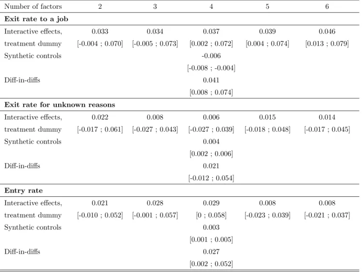
In Table 7, we report estimation results of the enterprise zone treatment e¤ect obtained with the

most promising methods that were evaluated in the Monte Carlo experiments.13 _{As explained at}

the end of the previous section, we use the interactive e¤ect model with a treatment dummy and the synthetic control approach, and contrast them with the most popular method of di¤erence in di¤erences.

Standard errors of the “Interactive e¤ect, treatment dummy” estimates are computed using independently and identically distributed disturbances, an assumption we justify below. More originally, we derive a con…dence interval for the synthetic control estimate which, as far as we

13_{The only slight modi…cation is that for the FGLS …rst di¤erence estimate, the covariance matrix is kept general}

know, has not been derived in the literature. We construct this con…dence interval by inverting a test statistic whose distribution is obtained by using permutation between local units under the (admittedly strong) assumption of independently and identically distributed disturbances across local units.

The procedure is as follows. Set the treatment e¤ect to 0 and substract this value to post

treatment outcomes of treated units. Next, draw 1000 times without replacement 13 units in the whole population (treated and controls) and consider them as the new treated units while the other 135 are the new controls. Construct synthetic controls in each sample and estimate treatment e¤ects. Derive from the empirical distribution of estimates the p-value associated to the null hypothesis that the treatment parameter is equal to zero. Inverting this test for di¤erent

values of 0 yields the con…dence interval that is reported in Table 7. In practice, we apply the

procedure for a large range of values for 0 around the estimated treatment e¤ect. Bounds of the

con…dence interval at the 95% level are the values of 0 at which the p-values are equal to 5%.

We analyze three outcomes at the level of municipalities constructed for each 6-month period between July 1993 and June 2003: exit from unemployment to a job, exit from unemployment for unknown reasons and entry into unemployment. The outcome describing unemployment exits (to a job or for unknown reasons) is de…ned as the logarithm of the ratio between the number of unemployed workers exiting during the period and the number of unemployed at risk at the beginning of the period. Entries are similarly de…ned. Table 7 reports results using our three estimation methods for each outcome.

Starting with exits to a job, we …nd a small positive and signi…cant treatment e¤ect using the interactive e¤ect method in line with the “Di¤-in-di¤s” estimate and with the …ndings in Gobillon et al. (2012) in which we used di¤erence in di¤erences but with a more limited number

of periods.14 _{The size of the interactive e¤ect estimate is slightly larger than the}

di¤erence-in-di¤erences estimate and tends to increase with the number of factors that are included in the estimation. In contrast, the “Synthetic control” estimate is negative and surprisingly quite precisely estimated.

[ Insert T able7 ]

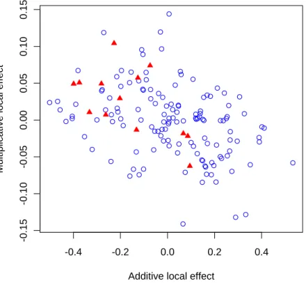
In the Monte Carlo experiment, those di¤erences were interpreted as an issue of disjoint

ports. We plot in Figure 1, the additive local e¤ect (i.e. the factor loading associated to the con-stant factor) and the multiplicative factor loading for each control unit (circle) and each treated unit (triangle) in the case where the model includes only two factors. This graph does not exhibit any evidence against the null hypothesis that the support of factor loadings for the treated units is included in the corresponding support for the controls. We tried to construct a test using per-mutation techniques (Good, 2005) and we failed to reject the null hypothesis of inclusion of the supports. In the absence of formal analyses of this test in the literature, we do not know however if this result is due to the low power of such a test.

[ Insert F igure1 ]

Another interpretation of the discrepancy between synthetic controls and interactive e¤ects would come from the presence of serial correlation. When a local e¤ect only is considered as in the di¤erence-in-di¤erences method, serial correlation is still substantial and the estimate of the auto-correlation of order 1 is around .35. In contrast, estimates of the serial auto-correlation in the interactive e¤ect model are close to zero. Factor models “exhaust” serial time dependence and this is also

true for spatial dependence.15 _{In contrast, we do not know much about the behavior of synthetic}

controls when serial correlation and spatial correlation are substantial. Interestingly, the within estimate without any correction for serial correlation is also on the negative side and close to the synthetic control estimate.

Results for other outcomes con…rm the diagnostic that synthetic control estimates seem to have a di¤erent behavior than interactive e¤ect and di¤erence-di¤erences estimates. While in-teractive e¤ect estimates of the treatment e¤ect are undistinguishable from zero when we analyze exits from unemployment for unknown reasons, di¤erence in di¤erences yield a positive but in-signi…cant estimate and synthetic controls a positive and in-signi…cant estimate. As we have reasons to believe that the treatment e¤ect should be larger for the outcome recording exits to a job than for the outcome recording exits for unknown reasons, synthetic control estimates seem incoherent. Nonetheless, it is true that synthetic control and interactive e¤ect estimates for the treatment

15_{This result is obtained using a Moran test when the distance matrix is constructed using the reciprocal of the}

geographical distance. Other contiguity schemes (for instance, when using discrete distance matrices constructed using 5 and 10km thresholds) capture positive spatial correlations although they diminish with the number of factors.

e¤ect on entries are very similar while di¤erence-in-di¤erences estimates seem too large.

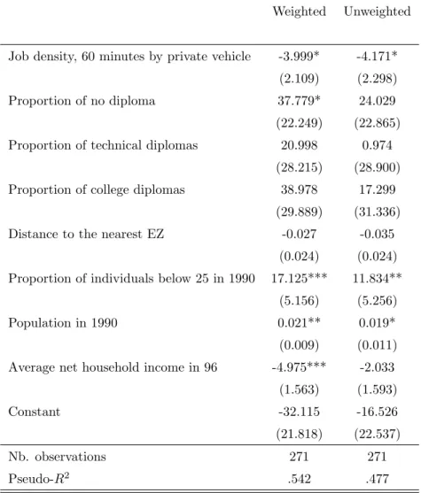
As a robustness check, we report in Table 8 the treatment e¤ect estimates when the propensity score is controlled for. In the interactive e¤ect and di¤erence-in-di¤erences approaches, this is done by including among the regressors the propensity score interacted with a trend t=T to mimic the presence of the propensity score in levels in the …rst di¤erence equation as in Gobillon et al. (2012). We also include the propensity score among variables used in the construction of synthetic controls. Results obtained using the method “Interactive e¤ect, treatment dummy”are very close to those obtained in the baseline case except when studying entries. The treatment e¤ect estimate is larger when the speci…cation includes four or less factors (including an additive one). Treatment e¤ects for the other outcomes – exits to a job and exits for unknown reasons – when using synthetic controls are now close to zero. Results obtained with di¤erence in di¤erences are similar to those obtained previously. In summary, once again, synthetic controls estimates are more sensitive to the speci…cation than factor models and di¤erence-in-di¤erences estimates. In conclusion, we have reasons to believe that interactive e¤ect estimates are more credible than other estimates in our application.

[ Insert T able8 ]

6

Conclusion

In this paper, we compared di¤erent methods of estimation of the e¤ect of a regional policy using time-varying regional data. Spatial dependence is captured by a linear factor structure that per-mits conditioning on an extended set of unobserved local e¤ects when applying methods of policy evaluation. We show how di¤erence-in-di¤erences estimates are biased and how linear factor meth-ods following Bai (2009) can be applied. We compare di¤erent versions of these interactive e¤ect methods with a synthetic control approach and with a more traditional di¤erence-in-di¤erences approach in Monte Carlo experiments. We …nally apply these methods to the evaluation of an entreprise zone program introduced in France in the late 1990s. In both Monte Carlo experiments and the empirical application, interactive e¤ect estimates fare well with respect to competitors.

There are quite a few interesting extensions worth exploring in empirical analyses.

First, there is a tension between two empirical strategies in regional policy evaluations (Blun-dell, Costa-Dias, Meghir and van Reenen, 2004). On the one hand, choosing areas in the