Individual growth model for the appendicularian Oikopleura dioica

HAL Id: hal-03002666

https://hal.archives-ouvertes.fr/hal-03002666

Submitted on 10 May 2021

HAL is a multi-disciplinary open access

archive for the deposit and dissemination of

sci-entific research documents, whether they are

pub-lished or not. The documents may come from

teaching and research institutions in France or

abroad, or from public or private research centers.

L’archive ouverte pluridisciplinaire HAL, est

destinée au dépôt et à la diffusion de documents

scientifiques de niveau recherche, publiés ou non,

émanant des établissements d’enseignement et de

recherche français ou étrangers, des laboratoires

publics ou privés.

Distributed under a Creative Commons Attribution| 4.0 International License

Oikopleura dioica

F Touratier, F Carlotti, G Gorsky

To cite this version:

F Touratier, F Carlotti, G Gorsky. Individual growth model for the appendicularian Oikopleura

dioica. Marine Ecology Progress Series, Inter Research, 2003, 248, pp.141-163. �10.3354/meps248141�.

�hal-03002666�

INTRODUCTION

Appendicularians are thought to play an important role in the flux of material throughout the water col-umn. This recent view emerges from the following characteristics: (1) most appendicularian species are capable of high grazing rates on a wide spectrum of particles, including microbial phytoplankton, bacteria and small detritus, and they are also able to utilise dis-solved organic matter (DOM) (Nakamura et al. 1997, Gorsky & Fenaux 1998, Gorsky et al. 1999); (2) their growth rates may be very high in situ (>10 up to 23 d–1_; Hopcroft & Roff 1995), i.e. 1 order of magnitude greater than those of copepods of equivalent body size; (3) appendicularians may outcompete copepods in regen-erative and microbial food web-based systems (Deibel 1998, Gorsky et al. 1999); (4) they could significantly increase and accelerate the export of carbon and asso-ciated elements (abandoned houses, fecal pellets, cadavers, and detritus (e.g. Alldredge 1976, Gorsky et

al. 1984, López-Urrutia & Acuña 1999); (5) dense pop-ulations of pelagic tunicates may deplete available food in a few days (Alldredge 1981, Deibel 1985); and (6) pelagic tunicates represent a single-step shunt between their small prey and their potential predators (chaetognaths, medusae, ctenophores, and fishes; e.g. Azam et al. 1983, Fortier et al. 1994, Gorsky & Fenaux 1998).

The overall objective of the EURAPP program (EURo-pean APPendicularians: www.obs-vlfr.fr/~eurapp/) was to improve our knowledge about the ecological role of distinct appendicularian species in representative mar-ginal seas of Europe, in relation to the flux of colloidal and particulate organic matter, and in relation to the structure, dynamics and resilience of important compo-nents in the marine plankton community as a whole.

The specific objectives of the present paper are to (1) describe the functioning of 1 appendicularian spe-cies at the organism level in controlled conditions; (2) build an individual growth model to simulate the © Inter-Research 2003 · www.int-res.com

*Email: touratie@univ-perp.fr

Individual growth model for the appendicularian

Oikopleura dioica

Franck Touratier

*, François Carlotti

_{, Gabriel Gorsky}

2_{Université Bordeaux 1, UMR 5805, Laboratoire d’Océanographie Biologique, Station Marine d’Arcachon,} 2, rue du Professeur Jolyet, 33120 Arcachon, France

3_{LOV, UMR 9073, Station Zoologique, Observatoire Océanologique, BP 28, 06234 Villefranche sur Mer, France}

ABSTRACT: A model of individual growth simulating the development of the main compartments and processes involved in the ecophysiology of the appendicularian Oikopleura dioica is presented. O. dioica is one of the 5 most frequent larvacean species inhabiting European seas, and laboratory

studies are available for comparison with model outputs. Individual growth and interactions with the external medium are described by state variables and fluxes of C and N, using the stoichiometric approach. Three forcing variables control the animal’s growth: temperature, food quantity, and food quality (i.e. C:N ratio and size of particles). Model outputs are compared to experimental data to analyse (1) the effect of food quantity and quality on trunk length; (2) the influence of temperature on trunk length, generation time, respiration, excretion and house production rate; (3) the variability of the filtration rate under different conditions of temperature, food quantity and food quality. Results of the model are coherent with most observations, and validation of the model was successful.

KEY WORDS: Appendicularia · Ecophysiology · Modelling · Carbon · Nitrogen Resale or republication not permitted without written consent of the publisher

evolution of compartments and processes involved in the ecophysiology of the individual; and (3) study the role of the individual in the transformation of elements and organic matter.

The species Oikopleura doica (Fol, 1872; Fig. 1a) was

selected for 2 reasons; (1) it is one of the 5 most repre-sentative species found in the European seas (Fenaux 1961, Acuña & Anadón 1992, Acuña et al. 1995), (2) it is one of the best known appendicularian species from

both in situ and laboratory studies. Given the

possibil-ity to maintain successive generations of this species in the laboratory (Fenaux & Gorsky 1985, Gorsky et al. 1987), experimental results are now available to build, calibrate and validate an individual growth model for this species.

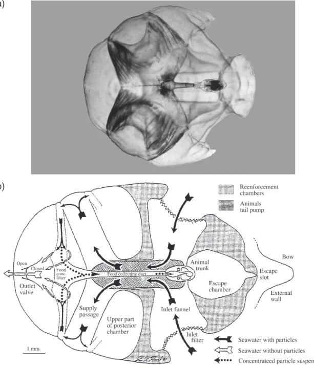
Details concerning the internal structure of the oiko-pleurid house (Fig. 1b) and its functioning can be found in Flood & Deibel (1998) and references therein. Fig. 1. (a) Oikopleura dioica (Fol 1872) inside its house (photograph by R. Fenaux; www.obs-vlfr.fr/~eurapp/). (b) Oikopleura labradoriensis. Diagram showing the internal structure and seawater circulation in the house; black arrows indicate water flow

through the house before, and white arrows after its passage through the food concentrating filter. The flow of trapped particles towards the mouth of the animal is indicated by the dotted arrows (after Flood & Deibel 1998)

a)

Oikopleura dioica uses its house to filter and

concen-trate food particles from the surrounding water. Undu-lating tail movements cause seawater to circulate through the house. During the feeding process ciliated spiracles on the floor of the pharyngeal cavity create the inflowing current that facilitates the introduction of food items into the pharynx (Gorsky 1980, Deibel & Powell 1987, Acuña et al. 1996). Before reaching the stomach, food particles undergo 3 different filtering processes. Large particles are excluded by the inlet filters, the digestible size particles are concentrated by the food-concentrating filter and are transported to the stomach by the pharyngeal filter. The inlet filter pore size of O. dioica is ca. 18 µm with a maximum

observed between 20 and 25 µm (Galt 1972, Deibel & Turner 1985, Flood & Deibel 1998). These filters, which are subject to clogging (the house must be abandoned in this case; Deibel & Lee 1992, Acuña et al. 1999), prevent large and potentially harmful par-ticles from entering the house. The pore size of the food-concentrating filter is much smaller (0.15 0.98 µm; Flood 1981), and this system is designed to concentrate the particles several hundredfold (Morris & Deibel 1993). Collected particles are then drained into the pharynx via the food collecting tube (Fig. 1b). Before being ingested, particles must be captured by the pharyngeal filter which is continuously secreted by the endostyle. Surprisingly, the pore size of this filter was observed to be larger than that of the food-concentrating filter in O. vanhoeffeni (Acuña et al.

1996). However, according to the latter authors, parti-cles smaller than the pharyngeal filter pore size could be retained not only by direct interception, but also by diffusional deposition.

The size of particles that are potentially ingested by

Oikopleura dioica ranges from 0.1 to approximately

25 µm (e.g. Flood 1978, Fenaux 1986), and the reten-tion efficiency generally exceeds 90% for particles > 3 µm (Deibel & Lee 1992, Gorsky et al. 1999). Dis-solved organic matter (DOM), bacteria, flagellates, pico- and nano-phytoplankton, amorphous particles (Alldredge 1981, Flood et al. 1992) are all potential food items for these animals which filter non-selec-tively (e.g. Gorsky 1980, Deibel & Turner 1985, Bedo et al. 1993). O. dioica individuals pump seawater

contin-uously, except when a new house is deployed (Deibel 1988, Gorsky & Palazzoli 1989), and they do not show any evidence of a diel feeding rhythm (Alldredge 1981).

METHODS

Overview of the Oikopleura dioica life cycle

The life cycle of appendicularians is simple com-pared to other zooplankton organisms such as cope-pods or other gelatinous organisms. Small differences among species exist, but the overall sequence of the life cycle remains the same. The simplicity and similar-ity of appendicularian life histories are advantageous when modelling their individual growth, population dynamics, and competition for resources.

Details concerning the life cycle of the genus Oiko-pleura can be found in Galt (1972), Fenaux (1976,

1998b), Paffenhöfer (1976), and Fenaux & Gorsky (1983). O. dioica is dioecious, in contrast to all other

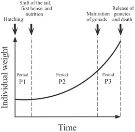
appendicularians, which are hermaphrodite. Accord-ing to Fenaux (1976), its life cycle is marked by 3 peri-ods separated by 4 significant events: fertilization, hatching, shift of the tail, and release of gametes. For this modelling study we consider, however, that the life of an individual is marked by hatching, shift of the tail, maturation of gonads and release of gametes (Fig. 2). Fertilization is not considered since we do not intend to model the population dynamics. The event termed ‘maturation of gonads’ corresponds to the period in the life cycle after which most of the available resources will be allocated to gametogenesis.

During Period P1, the trunk and the tail of the indi-vidual develop progressively; the indiindi-vidual is not able to filter seawater and consequently cannot ingest food particles. Its growth is negative, but the loss in weight is very small (Fenaux & Gorsky 1983). This period is also characterized by construction of the first house rudiment around the trunk. The mucus of this rudi-ment is secreted by the oikoplastic epithelium that occupies a large area (the oikoplastic region) above the mouth of the animal.

Time

Individual weight

Shift of the tail, first house, and

nutrition Maturation

of gonads

Release of gametes and death

Fig. 2. Oikopleura dioica. Overview of growth and of the

development periods (P1 to P3) modelled, which are de-limited by 4 events: hatching, shift of the tail, maturation

The shift of the tail is an important event in the life cycle, after which the pre-built house rudiment is deployed around the animal. The house is then used to filter seawater and concentrate particles prior to their ingestion. In the model, the duration of house deploy-ment is considered to be insignificant, which is a rea-sonable approximation given the fact that it takes only a few dozen seconds (Fenaux 1985, Gorsky & Palazzoli 1989). At the beginning of Period P2, the somatic cells reach their definitive number. The animal will there-after gain additional weight by increasing the volume of these polyploïd cells, and by investing new materials into the construction of gonads and production of gametes.

Development of the gonads accelerates during Period P3. Maturation of the reproductive cells is a pri-ority, since autolysis phenomena of oikoplastic and digestive cells have been observed at this stage. Auto-lysed material is apparently re-invested into the gonads (Gorsky 1980, Fenaux & Gorsky 1983). When gonads are mature, house rudiment secretion ceases since most oikoplastic cells are autolysed. The last house is abandoned just before the release of repro-ductive cells, a strategy that favours the dispersion of gametes. The sperm of male individuals is released through a spermiduct, whereas the oocytes of females are released by rupture of the ovary and genital cavity walls (Fenaux 1998a). In all cases, the death of animals occurs shortly after this event.

To survive during P1 and maximize reproductive potential at the end of P3, Periods P1 and P3 should be very short. In cultures of Oikopleura longicauda at

20°C, Fenaux & Gorsky (1983) showed that Periods P1, P2, and P3 last approximately 0.5, 6.16, and 1 d, respectively.

The symbols, descriptions and units of the 18 state variables of the present model are shown in Table 1, and information relative to the model parameters is given in Table 2. The model is built using several prin-ciples of the stoichiometric approach (see e.g. Sterner 1990, Touratier et al. 1999, 2001), which combines at least 2 elemental units (carbon and nitrogen in the present study) to compute variables and flows. The main advantage of this multi-currency approach is that both food quantity and food quality (C:N ratio) influ-ence the computation of the most important processes in the model.

Whatever the period considered thereafter, all C and N, continuous or discrete flows linking the state vari-ables of the model are represented in the connectivity matrix (Table 3).

Modelling Period P1

During Period P1, the animal must survive without feeding and build the first house rudiment from its own reserves. The state variables and processes used to

Symbols Descriptions Elemental unit x

DC Carbon weight of detritus accumulated on the inner wall of the working house C

DN Nitrogen weight of detritus accumulated on the inner wall of the working house N

EC Carbon weight of the gametes C

ENa Nitrogen weight of the gametes N

FC Carbon weight of the food outside the house C

FN Nitrogen weight of the food outside the house N

FPC Carbon weight of fecal pellets accumulated in the medium C

FPN Nitrogen weight of fecal pellets accumulated in the medium N

GC Carbon weight of the gonads C

GNa Nitrogen weight of the gonads N

HC Carbon weight of the working house C

HNa Nitrogen weight of the working house N

HFC Carbon weight of the food inside the house C

HFN Nitrogen weight of the food inside the house N

HRC Carbon weight of house rudiment C

HRNa Nitrogen weight of house rudiment N

ODC Carbon weight of detritus accumulated on the inner wall of old houses C

ODN Nitrogen weight of detritus accumulated on the inner wall of old houses N

OHC Carbon weight of old houses C

OHNa Nitrogen weight of old houses N

RC Carbon weight of respired products C

RN Nitrogen weight of excreted products N

SBC Carbon weight of structural biomass without the gonads C

SBNa Nitrogen weight of structural biomass without the gonads N a_{Not a state variable}

Table 3. Oikopleura dioica. Model connectivity matrix for all

carbon and nitrogen flows (in µg x ind.–1_bottle–1_d–1_{, where x}

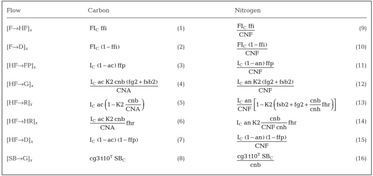
stands for C or N; d: continuous flows, m: discrete flows). Flows are defined as follows: [D→OD]x: detritus rejection; [F→HF]x: food intake; [F→D]x: accumulation of food on the inner wall of the house; [G→E]x: release of gametes; [H→OH]x: house rejection; [HF→FP]x: production of fecal pel-lets; [HF→SB]x: construction of structural biomass; [HF→G]x: construction of gonads from food; [HF→R]x: respiration/ excretion from food; [HF→HR]x: construction of house rudi-ment from food; [HF→D]x: accumulation of fecal pellets on the inner wall of the house; [HR→H]x: deployment of the house rudiment; [SB→G]x: construction of gonads from structural biomass; [SB→R]x: respiration/excretion from structural bio-mass; [SB→HR]x: construction of house rudiment from struc-tural biomass; [G→R]x: respiration/excretion from gonads

Description Symbols Values Units

Coefficient of the allometric equation for food intake at 0°C a 52.54a _pgC0.25_d–1

Carbon assimilation coefficient ac 0.67b _Wd

Nitrogen assimilation coefficient an 0.72b _Wd

Slope of the regression line between trunk length and temperature atl –50c _{µm (°C)}–1

Exponent of the allometric equation for food intake b –0.25d _Wd

Gonad construction rate from structural biomass at 0°C during P3 cg3 0.02 d–1

House rudiment construction rate at 0°C during P1 chr1 0.15 d–1

C:N ratio for the structural biomass, the gonads, and the gametes cnb 5.3e _{µgC (µgN)}–1

C:N ratio for the house rudiment, the working and the old houses cnh 250f _{µgC (µgN)}–1

Fraction of food intake available for ingestion ffi 0.95 Wd

Fraction of fecal pellet production released in the medium ffp 0.95 Wd Fraction of biomass production available for construction of the gonads during P2 fg2 0.1 Wd Fraction of biomass production available for construction of the house rudiment fhr 0.65 Wd Fraction of biomass production available for construction of the structural biomass fsb2 0.25 Wd during P2

Fraction of the house volume unoccupied by the organism fv 0.66g _Wd

Maximum net growth efficiency when assimilated food C:N ratio is equal to cnb k2m 0.44h _Wd

Half-saturation constant for the relationship representing the effect of forcing E ke 10000 µgC l–1

on ingestion

Half-saturation constant for food intake ki 240i _{µgC l}–1

Half-saturation constant for curve K2 kk2 1 µgC ind.–1

bottle–1_d–1

Respiration rate at 0°C during P1 res1 0.005 d–1

Size ratio between house diameter and trunk length rl 3.846j _Wd

10th root of Q10coefficient t10 1.1084c Wd

Food concentration threshold for maintenance tf 1 µgC l–1

Threshold for deployment of a new house (fraction of the sum SBC + GC) th 0.2376c Wd

Maximum trunk length at 23°C tlm 740c _µm

Threshold to enter period P3 (fraction of the maximum trunk length) ttl 0.8 Wd Sources: a_{Acuña & Kiefer (2000);} b_{Bochdansky et al. (1999);} c_{Gorsky (1980);} d_{Moloney & Field (1989);} e_{Gorsky et al. (1988);} f_{Alldredge (1976);} g_{Flood et al. (1990);} h_{Touratier et al. (1999);} i_{Hansen et al. (1997);} j_{Flood & Deibel (1998)}

Table 2. Oikopleura dioica. Growth model parameters. Wd: without dimension

Fx HFx FPx SBx Gx Rx HRx Hx Dx OHxODx Ex Fx d d HFx d d d d d d FPx SBx d d d Gx d m Rx HRx m Hx m Dx m

simulate this period are shown in Fig. 3. Just after hatching, the carbon weight of the animal (SBC; see Table 1) is initialised to that of the egg, whereas all other state variables in the model (Table 1) are set to zero. The carbon weight of the egg (0.013 µgC) is estimated assuming a diameter of 100 µm (range: 60 to 107 µm; Fenaux et al. 1986, Hopcroft & Roff 1995, Fenaux 1998b), and we then use the carbon weight –trunk length relationship provided by King et al. (1980) for Oikopleura dioica: log10(weight, µgC) = 2.6270 log10(trunk length, µm) – 7.1348.

We assume that the hypothesis of strict homeostasis is valid for appendicularians (i.e. their elemental com-position remains constant despite variable quality of the ingested food), as it has been shown to be the case in many other zooplankton groups such as copepods and cladocerans (see Touratier et al. 1999, 2001 and references therein). This assumption, which is partly justified by the absence of lipid storage in oikopleurids (Gorsky & Palazzoli 1989, Deibel et al. 1992), consider-ably reduces the number of state

vari-ables and highlights the structure of the present model. For instance, dur-ing Period P1 (see Fig. 3), variables SBN and HRN(Table 1) are not state variables since we assume that ratios SBC:SBN and HRC:HRN remain con-stant. These 2 ratios are parameters cnb and cnh in the model, respectively (Table 2). The value cnb = 5.3 µgC µgN–1was measured by Gorsky et al. (1988) for Oikopleura dioica and does

not differ much from that of other zooplankton groups such as copepods and euphausiids. Houses of appen-dicularians are primarily composed of mucopoly-saccharides (Körner 1952) with a very small nitrogen content relative to the carbon (Alldredge 1976). This means that parameter cnh is expected to be much higher than cnb. Alldredge (1976) determined the C:N ratio of 12 houses newly secreted by O. rufescens, and

she found a mean value for cnh of 250 µgC µgN–1_, which we use in the present study (Table 2). The large difference between cnb and cnh prevents the utilisa-tion of a single C:N ratio for the entire animal, as it is usually done when modelling other zooplankton groups. To describe the nitrogen compounds involved during Period P1, the state variable RN(Fig. 3, Table 1) is the quantity of excreted products (mostly ammo-nium; Gorsky 1980, Gorsky et al. 1987).

C and N flows during P1 are of 2 types (Fig. 3): con-struction of the house rudiment from structural bio-mass (symbolized by [SB→HR]x), and respiration or

excretion (i.e. [SB→R]_x), where the subscript x stands

for C or N unit (Table 3). All flows during P1 are con-tinuous (Table 3) and their parameterisation is shown in Table 4. Respiration [SB→R]C(see Eq. 1 in Table 4) during Period P1 depends on the ambient temperature (T), following a Q10of 3.51 (Gorsky 1980) of which the 10th root is computed (parameter t10 in Table 2). The construction of the house rudiment in carbon or [SB→HR]C(see Eq. 2, Table 4) follows similar rules of parameterisation. To ensure that the C:N ratio of the house rudiment will be equal to cnh, the nitrogen flow for construction of the house rudiment [SB→HR]Nmust be [SB→HR]Cdivided by cnh (Eq. 4 in Table 4). Ammo-nium excretion [SB→R]Nmust then be constrained by parameters cnb and cnh, as shown in Eq. (3) (Table 4), in order to satisfy the nitrogen mass conservation.

Modelling positive growth in Period P2

The carbon weight of the animal (WC) is defined here as the sum of the structural biomass (SBC) and the gonads (GC): SB_C HR_C R_C SB_N HR_N R_N

Carbon variables and processes

Nitrogen variables and processes

Continuous flow State variable Other variable

Fig. 3. Oikopleura dioica. Variables and processes used to

model Period P1 of the life cycle. Symbols and units are described in Tables 1–3

Flow Carbon Nitrogen

[SB→R]x res1 t10TSBC (1) (3) [SB→HR]x chr1 t10TSBC (2) (4) chr1 t10 SB cnh T C res1 cnb chr1 1 cnb 1 cnh t10 SB T C + _ − _   

Table 4. Oikopleura dioica. Carbon and nitrogen flows for period P1 (x stands

(1) A different definition could have been chosen (e.g. by adding to WC the weight of the house rudiment and/or that of the working house, which can be consid-ered as elements of the body), but WCis preferred for 3 reasons: (1) it corresponds to most measurements found in the literature for appendicularian individual weights; (2) at small timescales (h), WC is much less variable than WC+ HRC; and (3) WCis the input vari-able of the trunk length (TL; in µm) relationship pro-vided by King et al. (1980):

(2) The Oikopleura dioica individual enters Period P2 as

soon as the carbon weight of the house rudiment (HRC) reaches a critical weight (th WC), where parameter th (Table 2) represents a fraction of WC. For O. dioica, Gorsky (1980) found that the house represents as much as 19.2% of the animal’s overall carbon content, i.e. th = 0.2376 (Table 2); Deibel (1986 1988) found 10 to 36% for O. vanhoeffeni, and Alldredge (1976) gave a

range of 20 to 40%. When HRC≥th WC, the house rudi-ment HRCis deployed around the animal to become a working house called HC(Table 1, Fig. 4). As specified in Table 3, the deployment of a new house [HR→H]x

is a discrete event that occurs within the time step dt during model implementation, as follows:

if HRC≥(th WC) then

(3) (4) As for the house rudiment, the C:N ratio of the working house is kept constant (HC:HN= cnh).

The C and N quantities of the food available in the medium are FCand FN, respectively (Fig. 4, Table 1). The volume of seawater in the experimental bottle (V; in l) is used to compute the concentrations of food (FC:V and FN:V). When a new house is deployed, we assume that food concentrations inside and outside the house are the same. To compute the C and N weights of the food inside the house (HFCand HFN; Eq. 8 and Fig. 4), the volume unoccupied by the animal inside the house (VH) must be estimated. The house length HL (in µm; Eq. 5) is first deduced from TL (Eq. 2) assuming a constant size ratio rl = HL:TL of 3.846 (Table 2; see Flood & Deibel 1998). Considering that the shape of the house is spherical, we then compute its volume HS (in µm3_{; Eq. 6), from which VH is} deduced (in l; Eq. 7) using parameter fv (i.e. the frac-tion of HS unoccupied by the organism; Table 2) deduced from Flood et al. (1990) on Oikopleura van-hoeffeni.

HL = TL rl (5)

(6) (7) (8)

As soon as the first house is deployed, seawater fil-tration, food processing, and positive growth become possible. These processes depend largely on external conditions (food quantity and quality, temperature, etc.). All processes of the model during Period P2 are illustrated in Fig. 4. The maximum food intake rate (Im; d–1_{) is computed from the following allometric} equation:

(9) where parameters a and b are deduced from Acuña & Kiefer (2000), and Moloney & Field (1989), respectively (Table 2). The filtration rate F (l ind.–1_d–1_{) is then given} by: if E = 0 then F = 0 (10) (11) if E 0 then F Im W ki F / V C C ≠ = +( ) Im = a W 10( C 6 b) t10T HF F VH V and HF F VH V C C N N = = VH ₌ HS fv 10−15 HS 4 HL / 2 3 3 = π( ) HRCt+dt = 0 HCt+dt = HRCt TL 10 log W 7.1348 2.6270 10 C =  ( )+  WC = SBC+GC F_C HF_C SB_C G_C FP_C HR_C H_C D_C RC OH_C OD_C F_N HF_N SB_N G_N FP_N HR_N R_N H_N D_N OH_N OD_N

Carbon variables and processes

Nitrogen variables and processes

Continuous flow

State variable Other variable Discrete flow

Fig. 4. Oikopleura dioica. Variables and processes used to

model positive growth in Period P2 of the life cycle. Symbols and units are described in Tables 1–3

where E is the food retention efficiency of the pharyn-geal filter (the possible range of E is 0 to 1). When E = 0, the food cannot be retained by the pharyngeal filter and filtration is suspended (Eq. 10); when 0 < E ≤1 the food may be partially or totally captured by the pha-ryngeal filter and filtration is computed using Eq. (11). The half-saturation constant for food intake (ki = 240 µgC l–1_{; Table 2) is from Hansen et al. (1997). This} value agrees with the experimental work of Acuña & Kiefer (2000), who studied the functional responses of

Oikopleura dioca. The food intake FIC(µgC ind.–1d–1) is deduced from the filtration rate as follows:

(12) Once the food is inside the house, it can remain in suspension, be ingested by the animal or it can accu-mulate on the inner wall of the house. The food which is effectively ingested by the animal (IC; µgC ind.–1d–1) is calculated from the food intake FIC:

(13) where parameter ffi (Table 2) represents the fraction of the food intake available for ingestion. In the model, ffi = 0.95, which means that 95% of the food intake is available for ingestion, whereas the remaining 5% accumulates on the inner wall of the house. Gorsky (1980) and Gorsky & Palazzoli (1989) found that 25 to 37% of the material collected by appendicu-larians accumulate as detritus on the inner wall of the house; these higher percentages are explained by the fact that measurements were made on abandoned houses, in which the quantity of accumulated material (including feces) is largest.

From Eq. (13), 3 different cases may arise depending on the value of the retention efficiency E: (1) when E = 1, all filtered food (fraction ffi) is ingested since IC= FIC ffi; (2) when E = 0, IC= 0 since FIC= 0 (see Eqs. 10 & 12); and (3) when 0 < E < 1, the food concentration inside the house (HFC/VH) increases since IC > FIC ffi. According to Morris & Deibel (1993) and Acuña et al. (1996), the increasing concentration of food inside the house could favour the aggregation of particles, and thus result in an increase of the retention efficiency. In Eq. (13), we attempt to simulate this effect by using a Michaelis-Menten function where the food concen-tration affects the global retention efficiency (the term in brackets) through the difference (1 – E).

The respiration for maintenance (RBC; in µgC ind.–1 d–1_{) follows the parameterisation proposed by} Touratier et al. (1999) for copepods:

(14) where tf is the food concentration threshold for main-tenance (Table 2). Its value (1 µgC l–1_{) was deduced}

during model calibration. Ranges found in the litera-ture for the carbon assimilation coefficient (ac, Table 2) are quite large: 0.17 to 0.88 for Oikopleura dioica

(Gorsky 1980), and 0.42 to 0.83 for O. vanhoeffeni

(Bochdansky et al. 1999). From the latter, a mean value of 0.67 is used. In the present section, growth must be positive, i.e. the carbon contained in assimilated food must exceed the metabolic requirements for mainte-nance (ICac > RBC).

The parameterisation used for the C and N flows that characterise Period P2 when growth is positive (Fig. 4) is listed in Table 5. The nitrogen food intake (Eq. 9, Table 5) is computed from its carbon equivalent (Eq. 1, Table 5) by using the food C:N ratio (CNF = FC:FN). The food that accumulates as detritus (DC and DN) on the inner wall of the house is computed from Eqs. (2) & (10) (Table 5). The fraction ffp (Table 2) of the fecal pellets (FPC and FPN) produced by the animal is released to the medium (Eqs. 3 & 11, Table 5), whereas the remaining part (1 – ffp) accumulates as detritus on the inner wall of the house (Eqs. 8 & 16, Table 5). To com-pute the nitrogen flows, the nitrogen assimilation coef-ficient (an, Table 2) is set to 0.72 (Bochdansky et al. 1999).

Once assimilated, the food is used for production of new biomass and for respiration/excretion. The para-meterisation of these processes is based on the stoi-chiometric approach developed by Touratier et al. to simulate the influence of food quantity and quality on copepod growth (for details, see Touratier et al. 1999), with the following parameterisation for appen-dicularians.

Since ac ≠ an, the C:N ratio for assimilated food (CNA) differs from that for ingested food (CNF). The relationship between the 2 ratios is given by CNA = CNF(ac:an). The net growth efficiency K2, defined as the ratio of production over assimilation when CNA = cnb, is computed as follows:

(15) Variable K2 reaches a maximum value k2m when ingestion IC becomes saturating, and it is null when (ICac) = RBC. There is no estimate of k2m for appen-dicularians, so that we chose a value typical of cope-pods, 0.44 for k2m (Table 2) (Touratier et al. 1999).

During Period P2, the production of new biomass is the sum of 3 processes: production of (1) structural bio-mass SB (Eqs. 4 & 12, Table 5); (2) gonads G (Eqs. 5 & 13, Table 5); and (3) house rudiment HR (Eqs. 7 & 15, Table 5). The contribution of each process to total pro-duction is computed using the fractions fsb2, fg2 and fhr, which are equal to 0.25, 0.1 and 0.65, respectively (Table 2). These parameters are adjusted during model calibration, and 2 conditions must be satisfied

concern-K2 k2m I ac RB kk2 I ac RB C C C C = − + − RB Im tf ki tfW ac C = C + I FI ffi E 1 E HF / VH ke HF / VH C C C C = + −( ) ( ) +( )    FI FF V C C =

ing their values: (1) mass conservation must be respected (fsb2 + fg2 + fhr = 1), and (2) the gain in car-bon weight of the house rudiment (HRC) must be higher than that of the individual’s carbon weight (WC; see Eq. 1) since the deployment of a new house de-pends on the comparison between HRCand WC (see above). This is done by choosing fhr > (fsb2 + fg2).

Respiration and excretion are simulated using Eqs. (6) & (14) (Table 5), respectively. Mass conserva-tion for C and N after assimilaconserva-tion must be satisfied: by summing Eqs. (4) to (7) for the carbon cycle, and Eqs. (12) to (15) for the nitrogen cycle (Table 5), we obtain the assimilation of carbon (IC ac) and that of nitrogen (ICan:CNF), respectively. An important char-acteristic of appendicularians, however, is that cnh >> cnb (Table 2). In order to respect these ratios, it is assumed that the organism uses 250 (i.e. cnh) times less N than C during the construction of the house rudiment (compare Eqs. 7 & 15, Table 5). It follows that the resulting excess of N must be excreted to satisfy mass conservation (Eq. 14, Table 5).

The deployment of a new house consists in a sequence of discrete events that occurs as often as the house rudiment C content (HRC) reaches a threshold defined by the product (th WC):

if HRC≥(th WC) then

(16) (17) (18)

The full sequence of events consists of Eqs. (16) to (18), then followed by Eqs. (3) & (4) (see above). When a new house is being deployed by the animal, the old house (HC) and the detritus (DC and DN) are aban-doned. They accumulate in the medium as old houses (OHC) and old detritus (ODCand ODN), as parameter-ized in Eqs. (16) & (17) (see also Fig. 4). When the house rudiment (HRC) is deployed to become a work-ing house (HC; see Eqs. 3 & 4), there is no detritus (DC and DN are initialized to 0; Eq. 18).

In the model, Oikopleura dioica enters Period P3

when trunk length TL (Eq. 2) reaches a size threshold called TLMGON, computed as follows:

(19) Threshold TLMGON decreases with increasing tem-perature. This effect is represented by a negative slope (atl; Table 2). Values for parameters atl and tlm (the maximum trunk length at 23°C) were estimated from the experimental work of Gorsky (1980). Since the maximum TL of an individual (tlm) is observed just before the release of gametes, a fraction ttl (0.8, Table 2) is used to compute threshold TLMGON(Eq. 19).

Modelling positive growth in Period P3

Period P3 is characterized by development of gonads. The parameterisation used to simulate the processes involved during Period P3 (Table 6; see also Fig. 5) is similar to that used during Period P2, but with the following 3 differences:

TLMGON = [atl T( −23)+tlm ttl]

DCt dt+ = 0; DNt dt+ = 0

ODCt dt+ = ODCt +D ;Ct ODNt dt+ =ODNt +DNt

OHCt dt+ = OHCt +HCt

Flow Carbon Nitrogen

[F→HF]x (1) (9) [F→D]x (2) (10) [HF→FP]x (3) (11) [HF→SB]x (4) (12) [HF→G]x (5) (13) [HF→R]x (6) (14) [HF→HR]x (7) (15) [HF→D]x (8) I 1 an 1 ffp (16) CNF C( − )( − ) IC(1 ac 1 ffp− )( − ) I an K2 cnb CNF cnhfhr C I ac K2 cnb CNAfhr C I an CNF 1 K2 fsb2 fg2 cnb cnhfhr C ₋  _{+ +}      I ac 1 K2 cnb CNA C  −  I an K2 fg2 CNF C I ac K2 cnb CNAfg2 C I an K2 fsb2 CNF C I ac K2 cnb CNAfsb2 C I 1 an ffp CNF C( − ) IC(1 ac ffp− ) FI 1 ffi CNF C( − ) FIC(1 ffi− ) FI ffi CNF C FI ffiC

Table 5. Oikopleura dioica. Carbon and nitrogen flows for Period P2 when growth is positive (ICac > RBC) (x stands for C or N).

(1) The C and N used for production of structural bio-mass during Period P2 (Eqs. 4 & 12; Table 5) is utilised for production of gonads during Period P3 (Eqs. 4 & 12 in Table 6 are the sum of Eqs. 4 & 5, and Eqs. 12 & 13 in Table 5, respectively).

(2) Autolysis phenomena of oikoplastic and digestive cells have been observed during Period P3, indicating that some materials of the structural biomass are re-invested into the gonads. This new process is para-meterised by Eqs. (8) & (16) (Table 6). During Period P3

and positive growth, the structural biomass SB always decreases, whereas the individual weight WC (SBC+GC) always increases.

(3) Release of gametes is a discrete process (EC, the carbon content of the gametes, is released from the gonads GC; see Table 1 and Fig. 5) that occurs as soon as the trunk length of Oikopleura dioica reaches

threshold TLRG, which is defined as follows:

(20)

TLRG = atl T( −23)+tlm

Flow Carbon Nitrogen

[F→HF]x (1) (9) [F→D]x (2) (10) [HF→FP]x (3) (11) [HF→G]x (4) (12) [HF→R]x (5) (13) [HF→HR]x (6) (14) [HF→D]x (7) (15) [SB→G]x (8) cg3 t10 SB (16) cnb T C cg3 t10 SB T C I 1 an 1 ffp CNF C( − )( − ) IC(1 ac 1 ffp− )( − ) I an K2 cnb CNF cnhfhr C I ac K2 cnb CNA fhr C I an CNF 1 K2 fsb2 fg2 cnb cnhfhr C ₋  _{+ +}      I ac 1 K2 cnb CNA C  −  I an K2 fg2 fsb2 CNF C ( + ) I ac K2 cnb fg2 fsb2 CNA C ( + ) I 1 an ffp CNF C( − ) IC(1 ac ffp− ) FI 1 ffi CNF C( − ) FIC(1 ffi− ) FI ffi CNF C FI ffiC

Table 6. Oikopleura dioica. Carbon and nitrogen flows for Period P3 when growth is positive (ICac > RBC) (x stands for C or N).

Variables, parameters and flows are defined in Tables 1–3

Flow Carbon Nitrogen

[F→HF]x (1) (8) [F→D]x (2) (9) [HF→FP]x (3) (10) [HF→R]x (4) (11) [HF→D]x (5) (12) [SB→R]x (6) (13) [G→R]x (7) RB I ac G (14) SB G cnb C C C C C − [ ] + ( ) RB I ac G SB G C C C C C − [ ] ₊ RB I ac SB SB G cnb C C C C C − [ ] + ( ) RB I ac SB SB G C C C C C − [ ] ₊ I 1 an 1 ffp CNF C( − )( − ) IC(1 ac 1 ffp− )( − ) I an CNF C I acC I 1 an ffp CNF C( − ) IC(1 ac ffp− ) FI 1 ffi CNF C( − ) FIC(1 ffi− ) FI ffi CNF C FI ffiC

Table 7. Oikopleura dioica. Carbon and nitrogen flows for Periods P2 and P3 when growth is zero or negative (ICac ≤RBC)

When TL ≥TLRG, the sequence of discrete events is given by Eqs. (16) to (18) above, followed by Eqs. (21) to (23). The old house and the associated detritus are abandoned, but there is no new house (Eq. 21) as most oikoplastic cells are empty due to the autolysis.

(21) (22) (23)

Modelling zero or negative growth in Periods P2 and P3

When food concentration is very low, growth can be zero or negative. In the model, this occurs when the quantity of assimilated carbon is equal to or lower than maintenance requirements (ICac ≤RBC). This is simu-lated using equations of Table 7 that parameterise pro-cesses appearing in Fig. 6.

Food intake (Eqs. 1 & 8; Table 7), accumulation of food (Eqs. 2 & 9; Table 7) and fecal pellets (Eqs. 5 & 12; Table 7) on the inner wall of the house, and produc-tion of fecal pellets (Eqs. 3 & 10; Table 7) are para-meterised in the same way as during positive growth (see Tables 5 & 6).

The priority of metabolism is to satisfy the costs of maintenance, and we assumed that respired or ex-creted products may originate from food, structural biomass, and/or gonads (Fig. 6).

When the carbon contained in the assimilated food exactly meets the metabolic requirements of the ani-mal (IC ac = RBC), growth is zero and respiration is computed using Eq. (4) of Table 7. All assimilated nitrogen must then be excreted in the medium to main-tain the stoichiometry constant (Eq. 11, Table 7). Note also that respiration and excretion using C and N from structural biomass and gonads are all zero in this case (Eqs. 6, 7, 13, & 14; Table 7).

For negative growth (i.e. RBC>ICac> 0), all assimilated C and N from food is required for respiration and excre-tion (Eqs. 4 & 11, Table 7). There is not enough carbon, however, to meet all metabolic requirements, so that the organism must use carbon from its structural biomass and gonads, the contribution of each compartment being proportional to their weight (Eqs. 6 & 7, Table 7). The sum of Eqs. (4), (6) & (7) (Table 7) is equal to the respira-tion for maintenance (RBC). To maintain the stoichio-metry of SB and G constant, excretion is computed from respiration divided by ratio cnb (Eqs. 13 & 14, Table 7). When food assimilation is zero (ICac = 0), respiration and excretion using C and N from food are zero (Eqs. 4 & 11, Table 7). In this case, growth is still lower and the costs of maintenance must entirely be sustained by the C and N of SB and G (Eqs. 6, 7, 13 & 14; Table 7).

GCt dt+ = 0 ECt dt+ = GCt HCt dt+ = 0 F_C HF_C SB_C G_C HR_C H_C D_C RC OH_C OD_C F_N HF_N SB_N G_N HR_N R_N H_N D_N OH_N OD_N FP_C E_C FP_N E_N

Carbon variables and processes

Nitrogen variables and processes

Continuous flow Discrete flow

State variable Other variable

Fig. 5. Oikopleura dioica. Variables and processes used to

model positive growth in Period P3 of the life cycle. Symbols and units are described in Tables 1–3

F_C HFC SBC GC FP_C HRC HC DC RC OHC ODC F_N HFN SB_N G_N FP_N HR_N RN HN DN OH_N OD_N

Carbon variables and processes

Nitrogen variables and processes

Continuous flow State variable Other variable

Fig. 6. Oikopleura dioica. Variables and processes used to

model zero or negative growth in Periods P2 and P3 of the life cycle. Symbols and units are described in Tables 1–3

An important consequence of negative growth is that construction of the house rudiment is stopped. This means that as long as growth is zero or negative, the animal cannot deploy a new house. Another conse-quence of negative growth is that release of gametes cannot occur since individual weight (and hence trunk length) is decreasing.

The system of differential equations for the model is shown in Table 8. This system is resolved using the Runge Kutta 4th order method with a variable time step procedure.

RESULTS Behaviour of the model

The overall behaviour of the model was explored by choosing a set of 5 experimental conditions defined as ‘standard simulation’: (1) volume of the experimental bottle V = 0.04 l; (2) carbon weight of the food FC = 26 µgC; (3) nitrogen weight of the food FN = 4.57 µgN; (4) temperature T = 23°C; and (5) food retention effi-ciency of the pharyngeal filter E = 1. This set of exper-imental conditions (Expt 5, Table 9) was used by Gorsky (1980) to study the influence of temperature on trunk length of Oikopleura dioica. Among the 36 sets

of experimental conditions that we used later to test the model (Table 9), Expt 5 was chosen as the standard simulation, because growth of O. dioica is maximized

(one of the shortest generation times: 3.23 d from

hatching to release of gametes). Expt 5 is characterised by C and N food concentrations of 650 µgC l–1 _and 114.25 µgN l–1, respectively, and CNF = 5.68 µgC µgN–1_{, which is the Redfield ratio. The model is} designed to simulate the growth of only 1 individual contained in an experimental bottle. In permanent rou-tine cultures of appendicularian species (e.g. Fenaux & Gorsky 1985, Gorsky et al. 1987), animals are usually moved to a new bottle (at least once a day) where ini-tial food levels are restored. To keep track of products released or abandoned by the animal, our simulated individual was maintained in the same bottle, but the food level was reinitialised every day at the first time step after midnight. The simulation assumes that prod-ucts that accumulate in the bottle (old houses and detritus, CO2, NH4+) do not affect growth conditions. In standard simulation the duration of the life cycle from hatching to death is 3.23 d. The individual spends 4.1, 77.1, and 18.8% of its life in Periods P1, P2 and P3, respectively (Fig. 7). Similar percentages of 6.5, 80.4, and 13.1% were estimated by Fenaux & Gorsky (1983) for Oikopleura longicauda, despite different

experi-mental conditions.

Each day, larger quantities of food are filtered by the growing Oikopleura dioica (FC, Fig. 7a), but food quan-tity is never limiting. The carbon weight of fecal pellets (FPC) accumulates continuously in the bottle, reaching ca. 8 µgC at the end of P3 (Fig. 7a). Both the structural biomass (SBC) and the gonads (GC) increase during P2 (Fig. 7b). During P3, the construction of gonads is accelerated, whereas the structural biomass slowly decreases due to autolysis. At the end of P3, all gametes are released in the medium from the gonads and GC= 0.

The deployment of the house rudiments is illustrated in Fig. 7c. The carbon contained in the house rudiment (HRC) is regularly transferred to a new working house (HC). Each time, HRC becomes zero and HC increases by a step. Both HRC and HC increase pro-portionally to the individual weight, whereas the fre-quency of house renewal decreases. Detritus (DC) accumulates on the inner wall of the working house (HC) as soon as the new house is deployed (Fig. 7d). The abandoned houses and their associated detritus sink to the bottom of the experimental bottle to accu-mulate as old houses (OHC) and old detritus (ODC; Fig. 7e).

The respiration RC of the individual generates CO2 that accumulates in the bottle (Fig. 7f). The individual weight WC(Fig. 7g) is defined as the sum of SBCand GC(Fig. 7b), but in practice the individual weight mea-sured in laboratory may include the weight of the house rudiment and sometimes that of the house. TWC (= WC + HRC + HC) represents the upper boundary for the individual weight (Fig. 7g). Consequently, the d(DC)/dt = [F→D]C + [HF→D]C−[D→OD]C d(DN)/dt = [F→D]N + [HF→D]N−[D→OD]N d(EC)/dt = [G→E]C d(FC)/dt = −[F→HF]C−[F→D]C d(FN)/dt = −[F→HF]N−[F→D]N d(FPC)/dt = [HF→FP]C d(FPN)/dt = [HF→FP]N d(GC)/dt = [HF→G]C+ [SB→G]C−[G→R]C −[G→E]C d(HC)/dt = [HR→H]C−[H→OH]C d(HFC)/dt = [F→HF]C −[HF→FP]C −[HF→SB]C −[HF→G]C −[HF→R]C −[HF→HR]C −[HF→D]C d(HFN)/dt = [F→HF]N −[HF→FP]N −[HF→SB]N −[HF→G]N −[HF→R]N −[HF→HR]N−[HF→D]N d(HRC)/dt = [HF→HR]C+ [SB→HR]C−[HR→H]C d(ODC)/dt = [D→OD]C d(ODN)/dt = [D→OD]N d(OHC)/dt = [H→OH]C d(RC)/dt = [HF→R]C+ [SB→R]C+ [G→R]C d(RN)/dt = [HF→R]N+ [SB→R]N+ [G→R]N d(SBC)/dt = [HF→SB]C−[SB→G]C−[SB→R]C−[SB→HR]C

Table 8. Differential equations of the growth model of

measured individual weights should be somewhere between WC and TWC, depending on the presence/ absence of the house rudiment and house around the animal.

Food C:N ratio (CNF) is kept constant at 5.68 µgC µgN–1 _{during the standard simulation; fecal pellets} have a higher C:N ratio of 6.69 µgC µgN–1_{(Fig. 7h),} since an > ac (Table 2). C:N ratios for detritus (DC:DN) and old detritus (ODC:ODN) are equal (ca. 5.9 µgC µgN–1_{; Fig. 7i). Since detritus originates from food and} fecal pellets, its C:N ratio mirrors their relative contri-butions. During P1, the C:N ratio for respired over

excreted products is very low with RC:RN= 0.17 µgC µgN–1_{(Fig. 7j). The construction of the house rudiment} during P1 is a predominant process (Fig. 3 and Table 4) responsible for the extremely low value of RC:RN. Rela-tive to respiration, ammonium excretion is increased (excess N is eliminated) to maintain a constant cnh ratio in the house rudiment. Thereafter, during Periods P2 and P3, RC:RNincreases to about 3.5 µgC µgN–1due to the beginning of feeding large quantities of high quality food (i.e. CNF ratio). Nutrition affects respira-tion, excrerespira-tion, and their ratios. The elemental compo-sition of the structural biomass, of the gonads (i.e. cnb;

Study Expt V FC FN T E Source

Influence of food 1 0.1a ₂₆b _{4.57 23}a _{1 260 5.68 Gorsky (1980)}

level on TL 2 0.05a ₁₃b _{2.28 23}a _{1 260 5.68 Gorsky (1980)}

3 0.02a _5.2b _{0.91 23}a _{1 260 5.68 Gorsky (1980)}

4 0.005a _1.3b _{0.22 23}a _{1 260 5.68 Gorsky (1980)}

Influence of T on TL 5 0.04aa ₂₆b _{4.57 23}a _{1 650 5.68 Gorsky (1980)}

and generation time 6 0.04aa ₂₆b _{4.57 20}a _{1 650 5.68 Gorsky (1980)}

7 0.04a ₂₆b _{4.57 13}a _{1 650 5.68 Gorsky (1980)} 8 4 2563.2 451.42 5 1 640.8 5.68 Simulationc 9 4b ₂₁₄₄b _{377.59 7.5}a _{1 536 5.68 Paffenhöfer (1976)} 10 4b ₃₄₂₄b _{603.06 12}a _{1 856 5.68 Paffenhöfer (1976)} 11 4b _{2563.2 451.42 16}a _{1 640.8 5.68 Paffenhöfer (1976)} 12 4b _{2563.2 451.42 18}a _{1 640.8 5.68 Paffenhöfer (1976)} 13 4 2563.2 451.42 20 1 640.8 5.68 Simulationc 14 4 2563.2 451.42 25 1 640.8 5.68 Simulationc

Influence of food quality 15 0.1a _44.98b _{7.06 17}a _{1 449.8 6.37 Nin (1997)}

(C:N ratio) on TL 16 0.1a _44.98b _{4.49 17}a _{1 449.8 10 Nin (1997)}

Influence of TL on 17 0.125a _12.525b _{2.20 23.5}a _{1 100.2 5.68 Alldredge (1981)}

the filtration rate 18 1 52.5b _{13.12 13.5}a _{0.2 52.5 4 King et al. (1980)}

19 0.05a ₂₆b _{4.57 17}a _{1 520 5.68 Gorsky (1980)}

20 1b _53.92b _{9.49 13}a _{1 53.92 5.68 Paffenhöfer (1976)}

Influence of T and TL 21 0.25a _17.5b _{3.08 15}a _{1 70 5.68 Gorsky et al. (1987)}

on respiration 22 0.25a _17.5b _{3.08 20}a _{1 70 5.68 Gorsky et al. (1987)}

23 0.25a _17.5b _{3.08 24}a _{1 70 5.68 Gorsky et al. (1987)}

Influence of T and TL 24 0.1a ₇b _{1.23 15}a _{1 70 5.68 Gorsky et al. (1987)}

on excretion 25 0.1a ₇b _{1.23 20}a _{1 70 5.68 Gorsky et al. (1987)}

26 0.1a ₇b _{1.23 24}a _{1 70 5.68 Gorsky et al. (1987)}

Influence of T and 27 0.035 26 4.57 5 1 742.8 5.68 Simulationc

TL on the house 28 0.035 26 4.57 10 1 742.8 5.68 Simulationc

production rate 29 0.035a _{26 4.57 14}a _{1 742.8 5.68 Fenaux (1985)}

30 0.035a _{26 4.57 16}a _{1 742.8 5.68 Fenaux (1985)} 31 0.035a _{26 4.57 18}a _{1 742.8 5.68 Fenaux (1985)} 32 0.035a _{26 4.57 20}a _{1 742.8 5.68 Fenaux (1985)} 33 0.035a _{26 4.57 22}a _{1 742.8 5.68 Fenaux (1985)} 34 0.035 26 4.57 25 1 742.8 5.68 Simulationc 35 1 136.1a _{21.36 13}a _{1 136.1 6.37 Gorsky (1980)} 36 1 136.1a _{21.36 20}a _{1 136.1 6.37 Gorsky (1980)} a_{Data originates directly from the referenced paper}

b_{Data originates from the referenced paper, but a conversion factor is used to adapt the units to the present study} c_{Simulations used to increase the range of temperature tested with the model}

F F C N F V C

Table 9. Experiments used to validate the individual growth model of Oikopleura dioica. The 5 experimental conditions required

to run the model are: V, volume of seawater containing 1 individual (l); FC, carbon weight of the food (µgC); FN, nitrogen weight

of the food (µgN); T, temperature (°C); E, capture efficiency of the pharyngeal filter (without dimension). Other data shown: FC/V,

food concentration (µgC l–1_{); F}

Fig. 7. Oikopleura dioica. Results of the model for the standard simulation: (a) carbon weight of food (FC) and fecal pellets (FPC)

in the medium; (b) carbon weight of the structural biomass (SBC) and gonads (GC); (c) carbon weight of the house rudiment (HRC)

and of the working house (HC); (d) carbon weight of detritus accumulated on the inner wall of the working house (DC); (e) carbon

weight of abandoned houses (OHC) and of detritus accumulated on their inner wall (ODC); (f) carbon weight of respired products

(RC); (g) individual carbon weights (WCand TWC); (h) C:N ratio of food (FC:FN) and fecal pellets (FPC:FPN) in the medium; (i) C:N

ratio of detritus accumulated on the inner wall of the working house (DC:DN) and of abandoned houses (ODC:ODN); (j) C:N ratio

of respired to excreted products (RC:RN), and C:N ratio of the individual (TWC:TWN); (k) filtration rate (F); (l) carbon food intake

(FIC), carbon assimilation (ICac) and respiration for maintenance (RBC); (m) individual growth rate; (n) house production rate.

Table 2), and hence that of the individual (i.e. ratio WC:WN) remain constant. Ratio TWC:TWN, defined as (WC + HRC + HC) : (WN + HRN + HN), ranges from cnb to ca. 7.3 (Fig. 7j). This variability is induced mainly by the weight of the house rudiment (HRC; Fig. 7c) that changes the relative contribution of cnh within TWC:TWN.

The filtration rate F (Fig. 7k) computed from Eqs. (10) & (11) increases with WC(Fig. 7g). The jumps of F at the beginning of Days 2 and 3 are due to the daily restoration of the food level (Fig. 7a). The sudden vari-ation in the food level also affects food intake (FIC) and assimilation of carbon (IC ac), as shown in Fig. 7l. Growth is negative during Period P1, but it is positive during Periods P2 and P3 (Fig. 7m) since assimilated carbon always exceeds largely maintenance needs (ICac > RBC; Fig. 7l). Just after Period P1, the growth rate reaches a maximum of ca. 11 d–1_{. It then decreases} slowly to a minimum of ca. 2 d–1_{with the increasing} individual weight.

During the first day of the life period, 18 houses are produced by the animal (Fig. 7n). The rate is then lowered to 13 and 8 houses during Days 2 and 3, respectively.

From the standard simulation, a carbon budget can be drawn for the individual. From the 25.38 µgC of food filtered by the organism during the 3.23 d of its lifetime, 5.8% ends as detritus (ODC), 14% is in the form of old houses (OHC), 36% is respired (RC), 30% is ejected as faecal pellets, and 6.42% is invested into the eggs. The remaining 7.8% represents the cadaver of the individ-ual. A considerable amount of carbon is lost through respiration, but 58% of the carbon ingested by an indi-vidual may sink in the water column as large particles.

Comparison between observations and model output

Several experimental data sets for Oikopleura dioica

were used to test the response of the individual growth model. Experimental conditions and results of Gorsky (1980), Paffenhöfer (1976), Nin (1997), All-dredge (1981), King et al. (1980), Gorsky et al. (1987), and Fenaux (1985) are available to study (1) the influ-ence of the food level on individual trunk length (TL); (2) the influence of temperature (T) on TL and genera-tion time; (3) the influence of food quality on TL; (4) the influence of TL on filtration rate; (5) the influence of T and TL on respiration; (6) the influence of T and TL on excretion; and (7) the influence of T and TL on house production rate (see Table 9). Each of the 36 ments in Table 9 is characterized by a set of 5 experi-mental conditions (V, FC, FN, T, and E) often derived from the source paper. Table 2 provides the values for all parameters of the model.

Influence of food level on trunk length Expts 1 to 4 in Table 9 analyse the influence of the food level on TL. The primary goal of Gorsky (1980) was to determine the minimum food level required to allow positive growth and maturation of gonads. Results of these experiments are also presented by Gorsky & Palazzoli (1989). Seawater filtered by 50 µm, originating from the Bay of Villefranche (French Medi-terranean coast), was used for the cultures. In the 4 bottles containing 1 l of seawater each, 10, 20, 50, and 200 individuals (selected just after the shift of the tail) were cultured. Since the growth of only 1 individual is simulated by the model, the volume of seawater per individual varies accordingly (V, Table 9). The original units of the food level used by Gorsky (1980) are ‘µm3 food particles ind.–1_d–1_{’, which need to be transformed} into carbon equivalents. This is done by using a con-version factor of 200 µgC mm– 3_{proposed by Mullin et} al. (1966) for phytoplankton. Since the food supplied each day by Gorsky (1980) consisted of a mixture of phytoplankton species, we apply this factor to estimate the carbon weight of the food (FC, Table 9). From Expts 1 to 4, it must be noted that both V and FC decrease, but that food concentration FC:V remains constant (Table 9). The nitrogen weight of the food (FN) is also required to implement the model, but it cannot be estimated from the source paper. The Redfield C:N ratio of 5.68 µgC µgN–1_{is applied to compute F}

N. We thus assume that healthy phytoplankton was supplied in the cultures. The temperature (T) is kept constant at 23°C during the experiments, and we consider that all food particles could efficiently be retained by the pharyngeal filter (E = 1; Table 9).

The results of the simulations are shown in Fig. 8. As observed in the cultures, generation time increases with decreasing food levels. Observed and simulated maxi-mum TL remain constant however (ca. 750 µm). When simulating Expt 4 with the model, the individual was not able to reach threshold TLRG. This indicates that the food quantity of 1.3 µgC supplied each day was not enough to trigger the release of gametes. It is similar to the con-clusions of Gorsky (1980) and Gorsky & Palazzoli (1989) that the food level used during Expt 3 (26 ×106_µm3_food particles ind.–1_d–1_{, which corresponds to 5.2 µgC ind.}–1 d–1_{in the present study) was the minimum required to} induce the release of gametes.

Influence of temperature on trunk length and generation time

The experimental data sets originated from Gorsky (1980) and Paffenhöfer (1976). Simulations corre-sponding to those of Gorsky (1980) use Expts 5 to 7 as

experimental conditions (Table 9), where only the tem-perature T varies (23, 20, and 13°C, respectively). Sim-ilar conversion factors (volume of food particles to car-bon, and C:N ratio; see above) were used to estimate FC and FN. In these experiments, food concentration was much higher (FC:V = 650 µgC l–1). Increasing the food concentration is a good strategy to obtain satura-tion of ingessatura-tion, since FC >> ki, and thus to focus on the effect of temperature on growth only. The results of the 3 simulations are shown in Fig. 9a–c. When tempera-ture decreases, generation time and maximum trunk length TLRG increase. Although these characteristics are well reproduced by the model, it is clear that the model overestimates generation time and threshold TLRGin Expt 7. This may indicate that either the slope atl (Table 2) used in Eqs. (19) & (20) is underestimated, or that the life cycle of the cultured individuals (10 individuals in 0.4 l) was not yet completely finished, as discussed by Gorsky (1980).

Using seawater from the North Sea filtered through a 180 µm mesh, Paffenhöfer (1976) measured the

gen-eration time of Oikopleura dioica cultured under

vari-ous conditions of temperature (from 7.5 to 18°C). These data provide a good opportunity to test the behaviour of the present model, but many uncertainties exist on the conditions FCand FNto apply in the model. From the chlorophyll a (chl a) concentrations given by

Paf-fenhöfer (1976), we estimate FCby using a POC:chl a ratio of 400 µgC (µg chl a)–1_{. The utilisation of these} data is complicated by the fact that the exact number of individuals in the cultures is unknown. These uncer-tainties would be of less importance if the food levels were saturating. We cannot affirm it, but we assume it is true, given the large quantities of carbon present in the food, as deduced from the above approximations. The range of temperature used by Paffenhöfer (1976) was analysed using Expts 9 to 12, characterised by temperatures of 7.5, 12, 16, and 18°C, respectively. Since Oikopleura dioica is a species with worldwide

Fig. 8. Oikopleura dioica. Comparison between experimental

observations and model simulations: influence of food level on individual trunk length. Experimental conditions are listed

in Table 9

Fig. 9. Oikopleura dioica. Comparison between experimental

observations and model simulations: influence of temperature on individual trunk length. Experimental conditions are listed

distribution, it is interesting to extend the range of tem-peratures tested with the model. The effect of temper-atures as low as 5°C (Expt 8) and as high as 20 and 25°C (Expts 13 and 14, respectively) on the generation time were thus analysed. Results of the 7 simulations corresponding to Expts 8 to 14 and Paffenhöfer’s data are presented in Fig. 9d. The simulated generation times do not differ significantly from those observed by Paffenhöfer (1976). Given the very large range of tem-peratures tested (5 to 25°C), the simulated generation times may vary between approximately 2 and 40 d.

Influence of food quality (C:N ratio) on trunk length The influence of the elemental composition of sub-strates assimilated by bacteria or ingested by zoo-plankton, and the consequences on the overall struc-ture of food webs, are debated in the recent literastruc-ture (e.g. Urabe et al. 1995, Brussaard & Riegman 1998, Touratier et al. 2001). The sole data available on this topic for appendicularians are those measured by Nin (1997) in G. Gorsky’s laboratory at Villefranche sur Mer. Twenty Oikopleura dioica individuals cultured in

a bottle filled with 2 l of filtered seawater were fed with the small flagellate Isochrysis galbana cultured either

under nitrate unstarved or starved conditions. Expts 15 and 16 (Table 9) are designed to simulate the results of Nin (1997). The food quantity FCwas estimated using a specific conversion factor of 346 µgC mm– 3 _provided by Gorsky (1980) for I. galbana. Surprisingly, the food

C:N ratios for both starved and unstarved I. galbana

are not available for these experiments. Consequently, for nitrate unstarved I. galbana we assume a C:N ratio

of 6.37 µgC µgN–1_{, as recommended by Gorsky (1980).} For nitrate starved cells, we assume that a C:N ratio of 10 µgC µgN–1_{is an appropriate choice. The food} quan-tities FNfor Expts 15 and 16 were computed from FC and these ratios (Table 9).

Simulated results are compared to the observations in Fig. 10. The data of Nin (1997) show that when food quality decreases (i.e. increasing C:N ratio), the gener-ation time increases and TLRGis lowered. The model predicts that the generation time increases in response to a poor quality of the food, but unrealistic outputs are generally obtained: TLRG remains constant and the predicted generation times are much longer than observed. To improve the overall quality of the simu-lated results, we changed the value of the 2 parameters a and ki in the model (Table 2) to be more representa-tive of the specific prey (Isochrysis galbana). The

ex-perimental work of Acuña & Kiefer (2000) suggests that values of a = 49.51 pgC0.25_d–1_{and ki = 38.9 µgC l}–1 could be more appropriate to simulate the influence of this alga on growth of Oikopleura dioica. Better results

are obtained with the model using this specific set of parameters (Fig. 10), but the difference remains impor-tant. Concerning the generation time, it must be noted, however, that Nin’s data (Fig. 10a) are not always coherent with those of Paffenhöfer (1976): Fig. 9d shows that the generation time at 17°C (i.e. the tem-perature of Nin’s experiments) should be 8 or 9 d instead of ca. 5 d as in Fig. 10a. The reason for such a disagreement between the 2 studies is unknown.

Influence of the trunk length on the filtration rate The data sets of Alldredge (1981), King et al. (1980), Gorsky (1980), and Paffenhöfer (1976) were used to test the response of the present model to the filtration rate (Expts 17 to 20 in Table 9). Only the regression curves available from the original papers instead of the data themselves are presented here.

The in situ filtration rates of Oikopleura dioica were

estimated by Alldredge (1981) in the surface waters of the Gulf of California during July 1979. The volume of the feeding chamber containing 1 O. dioica was 0.125 l

(V of Expt 17 in Table 9). The averaged food concen-tration (POC) during the experiments was 120 µgC l–1_, but according to the author a mean of 83.5% passed through the incurrent filters of the house (see All-dredge 1981 for details). The food concentration avail-able for growth was thus 100.2 µgC l–1, which trans-lates to FC= 12.5 µgC (see Table 9). The quantity FN

Fig. 10. Oikopleura dioica. Comparison between

experimen-tal observations and model simulations: influence of food quality (C:N ratio) on individual trunk length. Experimental

was computed assuming that the C:N Redfield ratio is representative of the available food. The average tem-perature during the experiments was 23.5°C. The regression curve determined by Alldredge (1981) and the simulated results are presented in Fig. 11a. It must be noted, however, that in the experiments conducted by Alice Alldredge, several individuals of different sizes were enclosed separately in the chamber for the duration of the measurement only. The life history of these individuals is thus completely unknown, whereas the model simulates the development of an individual whose life history is completely known. The trunk length of individuals used by Alldredge (1981) was generally larger (600 to 1300 µm) than that com-puted with the model (< 715 µm). Among the factors analysed above (food level, temperature, and food quality), only the temperature could explain the differ-ence, since T and TL are inversely correlated (see ‘Influence of temperature on trunk length and genera-tion time’, and Fig. 9a–c). From this, we suspect that

the life history of the individuals used by Alldredge (1981) could have been marked by cold periods. Inter-estingly, the regression curve of Alldredge (1981) is in continuity with that computed by the model, which indicates that the simulated filtration rates could be realistic for small-sized individuals.

One objective of King et al. (1980) was to estimate the filtration rate of Oikopleura dioica when it was fed

with natural assemblages of free-living bacteria at Saanich Inlet, Canada. We assumed that the volume of 10 µm filtered seawater placed in the bottle was 1 l; this information is not given by King et al. (1980). The mean bacterial biomass reached 52.5 µgC l–1_{, and thus} FC= 52.5 µgC (see Expt 18 in Table 9). FNwas esti-mated from FC using a bacterial C:N ratio of 4 µgC µgN–1_{(Lancelot & Billen 1985). The temperature} dur-ing the experiments was maintained at 13.5°C. The capture efficiency E of the pharyngeal filter is roughly estimated at 0.2 (Table 9) from the particle size reten-tion spectra proposed by Acuña et al. (1996) for O. van-hoeffeni, considering that the size of bacterial cells

ranges from 0.2 to 2 µm (Painting 1989). As previously, the history of the individuals is unknown, but the sim-ulated results are coherent with the observations (Fig. 11b).

Gorsky (1980), using 50 µm filtered seawater from the Bay of Villefranche sur Mer, also provided estimates of the filtration rates for Oikopleura dioica, as represented

by the linear regression in Fig. 11c. Using the experi-mental conditions of Expt 19 (Table 9), the simulated results are in the range of the experimental data.

Finally, the filtration rates estimated by Paffenhöfer (1976) were simulated using the conditions of Expt 20 (Table 9) and seawater cultures of 4 l. We assumed that 4 individuals (the exact number is unknown) were used in each bottle, i.e. V = 1 l. The factor of Mullin et al. (1966) previously used to convert the volume of food particles into carbon equivalents was also applied to the original data, and FC= 53.92 µgC (Table 9). FNwas deduced from FC using the Redfield C:N ratio. The temperature was 13°C and E was set to 1. The differ-ence between the observed and the simulated rates is obvious, and it increases with body size. We suspect, however, that the present model is more realistic than Paffenhöfer’s data, since (1) the results of the present model are coherent with 3 other independent data sets (Fig. 11a–c); (2) King et al. (1980) and Gorsky (1980) already pointed out the overestimated filtration rates obtained by Paffenhöfer (1976), especially because the number of individuals present in the cultures could have been underestimated; and (3) it is unnatural that the maximum filtration rates obtained by Alldredge (1981) and Paffenhöfer (1976) should be similar (com-pare Fig. 11a,d) considering a difference in tempera-ture of 10.5°C between the 2 experiments (Table 9). Fig. 11. Oikopleura dioica. Comparison between

experimen-tal observations and model simulations: influence of individ-ual trunk length on filtration rate. Experimental conditions