Women's labour market participation interacting with macroeconomic growth and family policies

(1)

HAL Id: tel-00638278

https://tel.archives-ouvertes.fr/tel-00638278

Submitted on 4 Nov 2011

HAL is a multi-disciplinary open access archive for the deposit and dissemination of sci-entific research documents, whether they are pub-lished or not. The documents may come from teaching and research institutions in France or abroad, or from public or private research centers.

L’archive ouverte pluridisciplinaire HAL, est destinée au dépôt et à la diffusion de documents scientifiques de niveau recherche, publiés ou non, émanant des établissements d’enseignement et de recherche français ou étrangers, des laboratoires publics ou privés.

Women’s labour market participation interacting with

macroeconomic growth and family policies

Angela Luci

To cite this version:

Angela Luci. Women’s labour market participation interacting with macroeconomic growth and family policies. Economics and Finance. Université de Pau et des Pays de l’Adour, 2009. English. �tel-00638278�

(2)

Université de Pau et des Pays de l’Adour, France Université Augsburg, Allemagne

(cotutelle franco-allemande)

Thèse de doctorat en économie

Angela Stefanie GREULICH épouse LUCI

“Women’s labour market participation

interacting with

macroeconomic growth and family policies”

(« Emploi des femmes, croissance macroéconomique et politiques familiales.Quelles interactions ? »)

Directeurs de thèse : Prof. Jacques Le Cacheux,

Université de Pau et des Pays de l’Adour, France Prof. Anita B. Pfaff,

Université Augsburg, Allemagne Membres du jury: Prof. Jérôme Gautié,

Université Paris 1, France Prof. Jacques Le Cacheux,

Université de Pau et des Pays de l’Adour, France Prof. Anita B. Pfaff,

Université Augsburg, Allemagne Prof. Dominique Meurs, Université Paris X, France Date de la soutenance : 23 octobre 2009

(3)

Acknowledgements

First of all, I thank Professor Anita B. Pfaff and Professor Jacques Le Cacheux for their professional guidance, valuable critics and especially for their open-mindedness with respect to my research interests as well as for their continuous support beyond national borders. Furthermore, I thank Professor Stefan Klasen for his impetus that has enriched my research. In addition, this thesis has benefited greatly from helpful comments from and discussions with Hermann Gartner, Olivier Thévenon, Dominique Meurs, Johannes Jütting, Hélène Périvier, Nathalie Picard and Hannah Krieger. I thank them very much.

I have benefited from discussions and cooperation with participants of the research project “costs of children” for the European Commission, namely Olivier Thévenon (INED, Paris), Marie-Thérèse Létablier (CNRS/CES, Paris) and Antoine Math (IRES, Paris), which I want to thank very much.

Finally, I thank Jean-Noël for his continuous moral and emotional support and encouragement during this exciting research adventure.

Paris, June 2009

(4)

labour force is 54 percent, compared to over 80 percent male participation. According to the European Commission, across the 25 EU Member States in 2003, the employment rate for women was 55 percent compared to 71 percent for men. In many -not necessarily the poorest - regions of the world, women’s labour market participation is actually much lower than men's. This goes especially for mothers with young children. The ILO as well as the European Commission stress that women’s lower participation in the labour market exposes them to a higher risk of poverty and social exclusion. At the same time, the persisting gender employment gap is costly not only for women, but for the society as a whole. From an economic perspective, the gender employment gap represents a huge untapped source of potential talents. For this reason, one can say that the labour market loses a lot of valuable resources, the more so as women’s qualifications have increased continuously during the last decades. Consequently, one might suggest that in many countries, economic growth lies below its potential and an increase of female labour market participation would provide a considerable boost to the economy.

In order to prevent women from income poverty and to take advantage of women’s potential for the labour market, both the ILO and the European Union have set the target to raise female labour market participation significantly within the next years. To promote gender equality in decent work, the ILO has launched a Gender Promotion Programme (GENPROM) set up within the Employment Sector to enhance activities for gender mainstreaming in employment creation. The European Union has set the Lisbon target to increase female labour force participation to 60% in 2010, which involves a marked acceleration of the trend in the number of women at work when compared to previous decades, in particular for Mediterranean countries, which lag behind by far.

The political will to promote women’s labour market participation is backed up by the scientific finding that gender equality in terms of education and employment promotes macroeconomic outcomes. The finding seems intuitive, yet, it was observed only quite recently. Before 1950, in economics little attention was given to women’s and men’s different roles in the economy. In the 1960s and 1970s there was an increasing interest in women’s economic role because women’s labour market participation had continued to increase. Yet, this interest was primarily influential in microeconomics (process of intra-household decision

(8)

making, labour supply function). In macroeconomics, even today most models refer mainly to neoclassical determinants of economic development such as technology and the capital stock (along with institutions and trade) and do not have gender as an integral part of their analysis.

The present research offers a detailed investigation of the interactions between macro-determinants, gender aspects of the labour market and family policies. The first chapter discusses interactions between women’s labour market participation and GDP growth. The second chapter presents an empirical analysis of the impact of GDP on women’s labour market participation. The third chapter discusses the impact of family policies on mothers’ employment patterns in Europe, completed by a comparative case study for Germany and France.

More precisely, in the first chapter, concerning the link between GDP (growth) and female labour market participation, both theoretical and empirical findings are taken into account. The analysis shows that, whereas economists today agree that the impact of female labour market participation on GDP is strictly positive, the reverse impact of GDP on female labour market participation is not as clear.

Firstly, I show how endogenous growth models suggest a positive impact of women’s education and labour market participation on GDP due to their impact on a country’s human capital stock. In a next step, I show how empirical studies give evidence of the fact that gender discrimination in education and employment has a negative impact on GDP, which implies that gender inequality is costly to economic development. In the next step, I find out that, whereas a series of studies, theoretical and empirical ones, clearly prove that female labour market participation promotes GDP, economists today still disagree about the inverse impact of economic growth on female labour market participation. In the literature, one often finds the common assumption that economic development promotes gender equality. Yet, there are two different theoretical approaches, one that suggests a positive impact and another that suggests that GDP growth first lowers female labour market participation at

(9)

early stages of development and then increases it in the middle and long run. I demonstrate that recent empirical studies assume a convex impact of GDP on female labour market participation: that means that at intermediate income per capita levels, female labour market participation is lower than at low as well as at high levels of income per capita. By discussing measurement and estimation problems, I point out that the present time-series and cross-country studies do not globally confirm the assumed convex impact.

The first chapter reveals a research gap in this field, which is the empirical evidence of a convex impact of GDP on female labour market participation. Answering the question of whether there is a purely positive or rather a convex impact of GDP on female labour market participation is crucial. If GDP growth can have a negative impact on women’s labour market participation, simply trusting the equalising effects of economic growth is not advisable for policy makers who intend to effectively promote gender equality. If they do so, women’s potential remains underutilised, and this lowers a country’s growth performance.

Hence, the second chapter offers an empirical analysis that attempts to close this research gap.

The mutual interactions between GDP and female labour market participation present a particular challenge to the estimation model. The two-way causality between the variable “female labour market participation” and the variable “GDP” suggests that both variables are endogenous. This endogeneity problem means that the explaining variable is correlated with the error term in the regression model. Consequently, the estimated coefficients of the “exogenous” variable are biased and inconsistent. In order to address the endogeneity problem I use a large macro panel data set (combination of cross-country and time-series data), containing observations of over 180 countries that span over four decades. In contrast to the existing cross country studies, the use of macro panel data allows taking into account methodological problems caused by endogeneity. The applied empirical methods are: fixed

(10)

effects, 2SLS, System GMM, Moving Average and Granger Causality. I pay special attention to time-specific effects and distinguish between within-country and between-country variations. Furthermore, the larger data set allows testing for the robustness of the findings by using different specifications of the endogenous variable “female labour market participation”. My empirical work confirms a convex impact of GDP on female labour market participation, although no nation in the panel went through all stages. I point out that the informative value of the estimation results depends strongly on the availability and comparability of the used data. Missing data, especially for early time periods and developing counties may bias my estimation results. Furthermore, due to insufficient data availability, the estimation model is limited to only a few exogenous variables. This limits the insight provided by the estimation because the estimation model does not filter out the impact of several important macro-level determinants that vary over time, such as institutional variables like family policy instruments.

Chapter 3 singles out this aspect. In order to investigate the impact of family policies on female labour market participation, I focus the analytical scope on a cross-country analysis based on countries of the European Union and the recent decade. I expose the impact of family policies on female labour market participation in the EU (27) by paying special attention to the impact of the presence of children on women’s time dedicated to work by distinguishing between women’s full-time equivalent employment and part-time work as well as by taking into account the division of labour within European households.

The analysis shows that mothers’ employment patterns vary widely across European countries, with 11 countries forming extremes: in Denmark, Sweden and Finland, mothers tend to continue working full-time rather than reducing to part-time at the arrival of a child. In the Netherlands, the UK, Germany and Austria, the working activity of mothers shows a strong discontinuity (interruption, part-time work). In Spain, Italy, Greece and Malta, the labour market participation of mothers appears to be quite continuous at the arrival of a child because female employment rates are rather low in general. Furthermore, the analysis suggests that the impact of children on mother’ labour market participation is influenced by family policies. The discussed family policy instruments are cash support (benefits and tax

(11)

reliefs), child-rearing allowances during parental leave and childcare support. I point out that these instruments can impact women’s labour supply decision in a positive or a negative way, depending on the instruments’ characteristics. In some countries, the redistributive character of several family policy instruments risks discouraging mothers’ labour supply. It turns out that in Europe, one main challenge of family policy is to create a set of coherent family policy instruments that manage to simultaneously prevent families from income poverty and encourage mothers’ employment. This is in particularly valid for Germany, as the case study in the second half of the third chapter shows. This case study compares French and German family policy instruments. The focus on only two countries allows a closer examination of institutional details. I conclude that, whereas in France, most family policy instruments stimulate mothers’ labour supply more than in Germany, both countries’ tax systems significantly discourage mothers’ labour supply, and hence, reforms of the family taxation mechanisms are advisable.

(12)

Chapter I: The links between women’s economic empowerment and macroeconomic growth: theory and empirical evidence

Introduction

Equal status among men and women is a central developmental goal of many international bodies, for example UNICEF, ILO, the UN or the World Bank. The United Nations define gender equity as related to women's rights and economic development. In its 2001 report, “Engendering Development,” the World Bank formulates equal status as a goal that specifically benefits women and girls, as they bear the bulk of economic disadvantages of gender discrimination. The UN and the World Bank, however, also clearly demonstrate that inequality between men and women, particularly in terms of education, employment and income, is economically costly not just for women but also for all of society, because it limits a country’s economic growth and welfare. Consequently, the United Nations Millennium Project, for example, names gender equity as one of the key elements to end world poverty by 2015.

Recent theoretical and empirical studies in economic growth support the view that gender discrimination hinders growth. Naturally, quantity and quality of institutions, the degree of integration of trade and a country’s geography – particularly, its access to natural resources – have always been the key factors of income growth (cf. Rodrik, Subramanian and Trebbi, 2004). Yet, economists today agree that women’s economic empowerment significantly contributes to a country’s economic growth (c.F. Worldbank, 2001). Several theoretical and empirical economic studies ascertain a positive impact of women’s education, employment and income on growth and thereby suggest that gender differences in education, employment and income lead to high economic costs for society. The first part of this chapter gives an overview of these studies, which prove that a reduction of gender differences in education, employment and income would accelerate a country’s growth performance and therefore would raise aggregate welfare.

The second part of this chapter shows that the reverse impact of growth on the empowerment of women is much less researched and that the impact of growth on the economic status of women is not clear, neither in theory nor in terms of empirical analysis. Most available studies focus on the impact of growth on female labour market participation only. Intuitively, one would expect to find a strictly positive impact of growth on the female

(13)

labour market participation. This assumption is supported by a theoretical approach called the “modernisation neoclassical approach”, which is presented at the beginning of the second part. Yet, simply trusting the equalising effects of economic growth is not advisable for policy makers who intend to effectively promote gender equality in the labour market, because more recent studies acknowledge that the impact of growth on female labour market participation is not strictly positive. I present a series of theoretical arguments that suggest that growth convexly influences the female labour market participation, which implies a U-shaped pattern of female labour market participation along the economic development path. This means that at low income levels, income growth lowers female labour market participation relative to male labour market participation and increases it in the middle and long run only. This phenomenon is known as the “feminisation U”. Nevertheless, until today, empirical analysis gives no clear evidence, neither for the “modernisation neoclassical approach” nor for the “feminisation U” hypothesis. In the last part of the chapter, I discuss measurement and estimation problems which are the reason for the weak empirical findings. Finally, in exposing in detail what is scientifically known today concerning the interactions of macroeconomic growth and female labour market participation, this chapter discovers a research gap in the field of empirically analysing the impact of growth on female labour market participation.

(14)

1. Link one: The impact of women’s economic empowerment on macroeconomic growth

This section deals with a series of theoretical models and empirical studies that investigate the impact of women’s economic empowerment, that is, of women’s education, employment and income, on macroeconomic growth.

The first part shows how theoretical models illustrate the aforementioned growth impact. I start by elaborating how, during the evolution from exogenous to newer endogenous growth models, education (and, implicitly, accumulation of human capital) has gained increasing significance. Firstly, I present the central results of the exogenous growth model by Solow (1956). Then, I show how Barro and Sala-i-Matin (1995) endogenise a country’s growth by introducing human capital as an input factor, which allows modelling continuous long-term growth. Based on Knowles, Lorgelly and Owen (2002) I investigate how gender-specific distribution of education affects a country’s growth by pointing out that gender discrimination in education lowers a country’s growth potential. Based on Galor and Weil (1996) I illustrate how employment and earned income of women promotes growth over generations.

The second part of this section focuses on empirical estimations of the impact of women’s education, employment and income on macroeconomic growth. Firstly, I present how Barro and Sala-i-Martin (1995) estimate a negative impact of women’s education on growth, followed by a critical discussion of these puzzling estimation results, which is mainly based on Dollar and Gatti (1999) and Knowles, Logelly and Owen (2002). Drawing from Klasen (2002), I show that an improvement of the estimation method yields a positive impact of women’s education on a country’s national income level. Then, I show how Klasen (1999) empirically proves a positive impact of women’s employment on growth. Finally, I discuss Seguino’s (2000) estimations of the impact of women’s income on a country’s income level.

(15)

1.1. The impact of women’s empowerment on growth in theory 1.1.1. Exogenous growth according to Robert Solow

The enormous surge of economic growth in Western countries during the second half of the 20th century leads to the question as to how such growth can be secured for the long-term. Growth is usually measured as a long-term development of national income on the basis of change in per capita income. This takes the size of population into consideration. Still today, economists discuss determinants of a nation’s long-term growth. This is mainly because the variables that influence long-term growth trends differ considerably from those that cause short-term economic fluctuations.

Economist Robert Solow (MIT) formulated a model of growth for closed national economies that predicts a convergence of nations’ income levels. Solow’s model was first published in 1956 in the Quarterly Journal of Economics, and Solow won the Nobel Prize for it in 1987. Solow modelled a neoclassical production function, which establishes a relationship between aggregate output and input factors:

) , (K L F

Y = (1.1)

with Y: national income; K: capital; L: labour

The factors of production labour, L, and capital, K, determine national income, Y. The production factors’ constant returns to scale imply a doubling of output when both input factors double (hypothesis: linear homogenous Cobb Douglas production function). Output does not increase proportionally when only one input factor increases.

The declining marginal returns of L and K imply that an additional unit of input yields a larger increase in output at a low input level than at a high input level. The “Inada” constraint, typical for the Solow Model, states that the marginal returns of K and L approach infinity when K and L approach 0 and that the marginal returns approach 0 when K and L approach infinity.

(16)

The constant returns to scale allow us to write the production function with per capita terms: ) ( ) 1 , ( L f k L K F L Y = ⋅ = ⋅ (1.2) ) (k f y = ⇒ (1.3)

with Y: national income; K: capital; L: labour; y: per capita income; k: per capita capital stock

Equation (1.3) shows that growth of per capita income is determined by the growth of per capita capital stock. According to Solow, capital stock growth is in turn determined by savings, population growth and depreciations.1

One of the main implications of Solow’s growth model is that there exists a “Steady State” which is the long-term balance in which per capita terms no longer grow. For example, in a Steady State, the per capita capital stock’s growth rate is 0. Consequently, a nation’s aggregate output converges against its Steady State level. Furthermore, there is a Steady State Value k* for each savings rate value. Another noteworthy result of the model is the dynamic impact of the “Golden Rule” of the accumulation of capital: There exists a “golden” savings rate which maximises per capita consumption in the Steady State. When the savings rate lies under or above this value s*, the Steady State declines. Savings rates that are either too high or too low reduce per capita consumption: a savings rate that is too high directly hinders consumption possibilities and a savings rate that is too low slows down the mechanism of capital consumption indirectly with a time delay.

The Steady State exists due to the declining marginal returns of the input factors. Because population size L is exogenous, it is not possible for both input factors K and L to double simultaneously and an increase in K alone causes only a disproportionate increase in output Y. Hence, the Solow model of growth predicts that countries with capital stock values above the Steady State level will experience negative growth. Countries with a capital stock below the Steady State level, in contrast, will grow, although growth rates decline the closer the actual capital stock approaches its Steady State level. This is why a country’s growth has an inverse relationship with initial income: Wealthy countries with high per capita capital stock (but still below the Steady State level) grow less vigorously than poor countries. As a result, the per capita income of both countries converges to a common Steady State level.

1

(17)

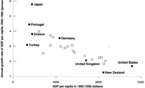
The graph in figure 1 shows in a comparison between OECD countries that there is an observable negative correlation between per capita income of countries during their beginning stages in 1950 and their growth rate up to 1992. Countries with low initial levels, such as Japan or Portugal, grow faster than, for example, the United States or Great Britain, which have had relatively high per capita incomes since the 1950s. The Federal Republic of Germany made up for the difference between its income and that of neighbouring countries after the Second World War and underwent a rapid accumulation of capital in the 1950s and 1960s. Blanchard (1999) underlines that, in comparison with other OECD countries, Germany’s slow-down in growth during the 1970s goes back in significant parts to the Solow effect (slowing of growth after a rapid beginning growth period).

Figure 1: GDP per capita in 1950 against GDP growth rate 1950 -1992

Source: Blanchard (1999)

However, an examination of countries outside of the OECD reveals that Solow’s growth model is not universally applicable. The model can be applied to four Asian tiger states: Singapore, Taiwan, Hong Kong and South Korea. Indonesia, Malaysia, China and Thailand also experienced strong rates of growth despite the Asian crisis of the 1990s. Still, in the poorest countries of the world, particularly in Africa, rapid growth and a convergence with the Western income level cannot be found. In Chad and Madagascar, the growth rate of per capita outputs has fallen approximately 1.3% per year since 1960 (cf. Blanchard, 1999). These examples suggest a conditional instead of an absolute convergence (cf. Barro und Sala-i-Martin, 1995): countries with similar savings rates, population growth and depreciation terms share a similar Steady-State level. Hence, a convergence of income seems only applicable to countries with homogenous parameters and similar economic structures.

(18)

Solow’s exogenous growth model can not explain what influences a country’s specific Steady State level. Empirical research on growth calculates that approximately 60% of a country’s actual growth cannot be described by the Solow model („Solow-residual“) (cf. Blanchard, 1999).

Economists, therefore, investigate alternate growth determinants that are not included in Solow’s growth theory. In a first step, an exogenous progress in technology, t, that saves capital K and labour L, was added to the model by Solow himself. A capital- and labour-saving progress in technology requires less capital and labour to maintain the same output. If production continues at the same rate, output will increase.

The new production function is:

) , , (K L t F Y = (1.4)

with Y: national income; K: capital; L: labour; t: technological progress

The modelling of technological progress as a third production factor shows that the per capita growth rate in a Steady State is the same as the rate of technological progress Yet, this model is also unable to explain the real reasons for an increase in income, because technological progress is considered exogenous. It was not until the 1980s that endogenous growth models were developed to explain long-term growth of productivity.

1.1.2. Endogenous growth: human capital as growth determinant

Robert Lucas and Paul Romer primarily developed a new endogenous growth theory during the mid 1980s. They endogenise technological advancement by integrating human capital as a third input factor in the production function. This significantly improved the empirical evidence of the growth model.

Barro und Sala-i-Martin (1995) further developed this approach. They endogenise technological advancement by splitting capital between physical capital, K, and human capital, H.

(19)

The production function is: ) , (K H F Y = or       ⋅ = K H f K Y (2.1)

with Y: national income; K: physical capital; H: human capital

There is an important difference between exogenous and endogenous growth models: in the aforementioned exogenous growth model, the second input factor next to capital, K, is labour, L, which is determined by population size. But L is not reproducible, as Solow assumes that a country’s population size does not change and cannot simply be changed. With an exogenous L, output growth can only be achieved by growing K, but the falling marginal returns of K result in a country’s income convergence in the Steady State.

The key feature of the endogenous model is that both input factors, K and H, can grow simultaneously. They are both considered endogenous and, therefore, reproducible. A simultaneous increase of K and H doubles output (constant returns to scale) and makes continuous growth without income convergence in the Steady State possible.2

With perfect competition, returns in physical and human capital equal their respective marginal product: K R K H f K H K H f K Y =       ′ ⋅       −       = ∂ ∂ (2.2) H R K H f H Y =       ′ = ∂ ∂ (2.3)

As K and H are substitutable, in the equilibrium the net earnings for both kinds of capital are:

r

R

_K

−

δ

_K

=

_H

−

δ

_H

=

(2.4)

with r as interest rate (market price of capital) and

δ

_i as depreciation rate of K and Hresprectively.

Equation (2.4.) determines a single, constant relationship K H _. If       = K H f

A with A as a constant, equation (2.1.) implies: AK

Y = (2.5)

2_{Furthermore, it seems plausible for H to assume constant marginal returns or even increasing marginal returns due to learning}

(20)

In this simplified model, H is not produced independent of K by education, for example. Rather, it is assumed that capital investment implicitly raises human capital (cf. Romer, 1986).

Hence, a change in either A or K directly affects Y. This means that, when population size remains constant, Y will grow constantly at the growth rates of K andH.

A more detailed, modified AK-model by Barro and Sala-i-Martin (1995) obtains the same result. The economists take a Cobb-Douglas production function with the input factors A (technological level of a country), K and H and combine it with optimising behaviour of households and companies:

α α − = 1 H AK Y (2.6)

This function also yields diminishing returns when K or H is increased separately, and it yields constant returns when K and H increase at the same time.

The rate of depreciation δ is assumed to be identical forK andH.

Output can be spent on consumption C and on investment in K and H (

I

_K and

I

_H).

Hence, the budget constraint for the national economy is:

H K I I C H AK Y = α 1−α = + + (2.7)

Change in both capital stocks is given by:

K I K° = _K −

δ

(2.8) H I H° = _H −

δ

(2.9)

Drawing from the Ramsey growth model of 1928, Barro and Sala-i-Martin (1995) now integrate the optimisation process of households into the model. The households chose consumption C and savings S so that their utility is maximised under the intertemporal budget constraint. This raises the problem of dynamic optimisation within time: a utility function should be maximised subjecto to constraints, but these constraints are dynamic, since they describe economic development over time (changes in K and H).

(21)

Therefore, the current utility function, u, which depends on the level of consumption, C, is discounted with the following time-preference factor:

t

e−ρ (2.10)

with time preference rate

ρ

>0.

The present value of the benefits is smaller the later the benefits ocurr.

The function that is to be maximised in a dynamic intertemporal case is called “Hamilton” function (analogous to the “Lagrange” function in the static case).

It reads: ) ( ) ( ) (C e I K I H u J = ⋅ −ρt +

υ

⋅ _k −

δ

+

µ

⋅ _H −

δ

) (AK H1 −C−I_K −I_H +

_ω

α −α (2.11)

ω, υ and µ are dynamic Lagrange multipliers.

υ and µ represent the actual shadow price (opportunity costs) of K and H and describe a change in the Hamilton function’s value due to a change in the capital stock (one unit). This is the value resulting from an increase in K or H, occurring at time t and expressed in utility units at time 0. The Hamilton function captures the overall effect of the level of consumption on utility. This is because the function takes into account that C directly affects u(C) and indirectly affects υ, as the level of consumption influences the changes in K and H.

The utility function is specified as follows:

)

1 (

)

1 (

)

(

1

θ

−

=

C

−

C

u

(2.12)

With 0〉

θ

〉1 as the constant elasticity of the marginal utility. The elasticity of the substitution for this utility function is the constant1

_θ

. The utility function, therefore, has the property of CIES (constant intertemporal elasticity of substitution). The larger θ is, the more the marginal utility will fall when C increases: households prefer today’s consumption over that of tomorrow.

The first derivatives of the Hamilton function J with respect to C,

I

_K and

I

_H will now be set equal to 0 to derive the optimality conditions.

(22)

°

υ

, and

°

µ

will be equated with the net marginal products of capital K J ∂ ∂ and H J ∂ ∂ .

These first order conditions define the household behaviour in the optimum (consumption path), just like they do in the case of static optimisation. When inserting the results in the budget constraint and performing some simplifications, one obtains the following growth rate of consumption:         − −       ⋅ ⋅       = − −

ρ

δ

α

θ

γ

c α K H K A ) 1 ( 1 (2.13) with _K H K A

α

δ

α −       ⋅ − − ) 1 (

as net marginal product ofK.

The difference between the net marginal product of K and

ρ

determines whether households choose a bundle of consumption that increases, stays constant or decreases over time. The greater

ρ

is in relation to the net marginal product, the greater is the current consumption, the less is invested, and the lower is the growth of future consumption. A large elasticity of marginal utility θ also limits consumption growth.

The second first order condition of the Hamilton function reveals that the net marginal product of human capital equals the net marginal product of physical capital:

δ

α

δ

α

α α −      ⋅ − ⋅ = −       ⋅ − − H K A H K A (1 ) ) 1 ( (2.14)

This implies that the relationship between both capital stocks can be represented as:

α

− = 1 H K (2.15)

This yields an identical net rate of return for H and for K: r*

δ

α

_⋅

₋

α

₋

=

(1− )

)

1 (

*

A

r

, (2.16) which is constant.

(23)

This implies: The ratio

H

K _{is constant, which means that}_K_and_H_{actually do grow at the same rate.}

Output grows at the same rate.

Moreover, equation (2.13) implies that consumption growth also is constant and equal to:

[

α

δ

ρ

]

θ

γ

__⋅ α _⋅ ₋ α ₋ ₋      = (1− ) * ) 1 ( 1 A (2.17)

The following applies to output:

) 1 (

1

α

−













−

⋅

=

AK

Y

(2.18)

The growth rate of K and H corresponds to the growth rate of Y andC. All growth rates correspond to

γ

∗.

This is how Barro and Sala-i-Martin use their endogenous growth model to prove the impact of investments in human capital on economic growth.

They also show that the restrictions

I

_K and

I

_H

≥

0

lead to an important result: The growth rate of output increases the more the actual value of

H

K _{and the Steady State value of}

H

K _{deviates. This goes for the two sorts of deviations: It has been empirically proofed that}

a small H

K _{-value (relative to the Steady State level) causes a lot of growth – for example,}

when a war destroys a significant amount of physical capital, but human capital remains intact. At the same time, a high

H

K _{-value (relative to the Steady State level) also promotes}

growth – for example, during an epidemic, the majority of infrastructure remains intact.

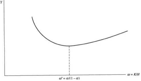
However, the graph in figure 2 illustrates how growth slows down when a national economy has more physical than human capital.

(24)

Figure 2 : Aggr. income growth in relation to the ratio physical / human capital

Source: Barro and Sala-i-Martin (1995)

A high H

K _{-value implies high costs of adjustment, as the process of building human capital}

is costly and time consuming. The fact that a national economy can recover more quickly from a shortage of physical capital than from a shortage of human capital proves the importance of investments in research and development, in education and in advanced training for promoting long-term growth.

Yet, advances in technology offer poorer countries the opportunity to grow. The rapid growth that took place in Asian tiger states, for example, occurred despite a relatively low physical capital base, because innovations in production could be cheaply imported from abroad (imitations). However, at the same time in Asian countries human capital levels were relatively high in comparison to developing countries in sub Saharan Africa, for example. Hence, developing countries would be immensely helped if they had both easier access to already-existing knowledge and more investments in education and professional training.

1.1.3. The impact of women’s education on growth

Knowles, Lorgelly and Owen (2002) try to answer how gender-specific dispersal of human capital influences a country’s growth. They use a neoclassical model of growth that uses female and male education as separate explanatory variables to clarify the impact of gender discriminating distribution within a national economy. Their model suggests that investments in women’s human capital have a positive impact on a country’s productivity and growth.

(25)

The model takes into account long-term effects of education by including the output elasticity of female and male human capital as well as of physical capital. Knowles et al. (2002) also model coefficients that represent differences in education between men and women.

The aggregate production function is:

(

)

α β β ψ ψ β β α − − − −

=

f m f m it it it it it it it

K

EF

EM

X

T

L

Y

1 (3.1)

EF stands for education of women, EM for education of men andX for health related capital. T stands for the technology level andL for the labour force of a country i at time t.

The production factors of the Cobb-Douglas production function all have constant returns to scale and positive, declining marginal returns. It is assumed that all countries have the same elasticities:

α

,

β

_f,

β

_m and

ψ

. These elasticities represent the percentage change in output associated with every 1% change in input. The elasticities lie between 0 and 1. When the elasticities add up to 1, the returns to scale are constant. In that case, the Cobb-Douglas function is linear homogeneous.

All variables are divided by T⋅L in order to achieve a production function that contains the output quantity per effective labour force:

ψ β β α it it it it it

k

ef

em

x

y

=

f m (3.2)

Labour force and technology are assumed to increase over time:

t n i it i e L L = ₀ (3.3) gt i it T e T = ₀ (3.4)

with n_i as growth rate of a country’s labour force and g as growth rate of technology, which is assumed to be uniform for all countries.

(26)

The growth rates of the factors of production k,ef_it,em_it and x_it are given as:

(

i

)

it it ki it s y n g k k = − + +

δ

° (3.5)

(

i

)

it it efi it

s

y

n

g

ef

°

=

−

+

δ

(3.6)

(

i

)

it it emi it s y n g em em° = − + +

δ

(3.7)

(

i

)

it it xi it s y n g x x° = − + +

δ

(3.8)

with s_ki,s_efi,s_emi and s_xias shares of output (i.e. the savings rates) that are invested in

it it em

ef

k, , and x_it (with total savings S equal to investments I).

δ

is the depreciation rate, which is the same over time and in all countries. The expression −gk_i describes the following relationship: with advances in labour-saving technology, labour efficiency units increase while the number of workers remains the same. These additional units must be endowed with capital. Net investments, measured per efficiency units of workers, are reduced by population growth. It becomes clear that k would fall according to the rates

n

,

δ

and gif s=0.

In the Solow model, the Steady State is defined by a constant capital stock per labour in units of efficiency. This is the case whensy(k*)=(n+g+

δ

)k*.

With

α

+

β

_f +

β

_m+

ψ

<1, equations (3.5) - (3.8) and (3.2) imply that in the Steady State:

η ψ β β ψ β β

δ

1 1         + + = − − − ∗ g n s s s s k i xi emi efi ki i m f m f (3.9) η ψ β ψ β α α

δ

1 1













+

=

− − − ∗

g

n

s

ef

i xi emi efi ki i m m (3.10) η ψ ψ β α β α

δ

1 1         + + = − − − ∗ g n s s s s em i xi emi efi ki i f f (3.11) η β β α β β α

δ

1 1         + + = − − − ∗ g n s s s s x i xi emi efi ki i m f m f (3.12) with

η

=1−

α

−

β

_f −

β

_m −

ψ

.

(27)

Because k_i∗,ef_i∗,em_i∗ and x∗_i are constant in the Steady State, the Steady State output per labour forcey_i∗ also remains constant.

By inserting equations (3.4) and (3.9) to (3.12) into equation (3.2), by logarithmising and converting, one arrives at:3

(

)

( )

efi f ki i i it it s s g n gt T L Y ln ln ln 1 ln ln ₀

η

β

η

α

δ

η

+ + + + − − + =       ∗

( )

emi

( )

xi m s s ln ln

η

ψ

η

β

₊ + (3.13)

The logarithm is used to obtain a linear relationship. Equation (3.13) represents the output per worker in the Steady State as a function of the respective savings rates of the factors of production.

When inserting the equation of the respective savings rates (that can be obtained by equations (3.10) to (3.12) in equation (3.13), one obtains a function that represents the output as a function of the Steady State sizes of the variables education and health.

(

)

( )

∗ ∗ − + − + + + − − + =       it f ki i i it it _T _g _n _g _s _ef L Y ln 1 ln 1 ln 1 ln ln ₀

α

β

α

δ

α

( )

∗

( )

∗ − + − + it it m x em ln 1 ln 1 α ψ α β _(3.14)

Human capital influences growth by means of its effects on the level of output per worker in a Steady State, which, in turn, influences its growth rate. Consequently, the elasticities of changes in output level as well as in output growth are important.

By substituting the growth rate of technologyg with constant

a

and the residual

ε

_i one arrives at:

( ) (

)

(

)

( )

∗ ∗ − + + + − − + + =       it f i ki i it it ef g n s T a L Y ln 1 ln ln 1 ln ln ₀ α β δ α α

( )

it

( )

it i m _em _x ε α ψ α β + − + − + ∗ _ln ∗ 1 ln 1 (3.15) 3_since

_Y

_L

=

_Ty

(28)

Education coefficients are positive if

β

_f,

β

_mand

α

are between 0 and 1.

The following algebraric rearrangement provides a basis for interpreting the impact of gender-specific differences in education ln

( ) ( )

em_it∗ −lnef_it∗ on a country’s output:

( ) (

)

(

)

( )

∗ ∗ − + + + + − − + + =       it m f i ki i it it ef g n s T a L Y ln 1 ln ln 1 ln ln ₀ α β β δ α α

( ) ( )

(

it it

)

( )

it i m _em _ef _x ε α ψ α β + − + − − + ∗ ∗ _ln ∗ 1 ln ln 1 (3.16)

It becomes apparent that, when

β

_mand

α

lie between 0 and 1, the elasticity of differences in education

α

β

− 1 m _{is positive.}

This should be interpreted as follows: Given a fixed level of female qualification, an increase in male qualification increases the output. On the other hand, if the female educational level increases while the male level remains unchanged, the difference decreases. This shows a negative effect on account of the positive coefficient.

Yet, the interpretation of the coefficient has its limits in this model, because the coefficient simply expresses the output elasticity of male education and

α

, and it leaves

β

_f unaccounted for.

The interpretation has also limits in the following model in which education refers to male education as well as the gender difference in education:

( ) (

)

(

)

( )

∗ ∗ − + + + + − − + + =       it m f i ki i it it _a _T _s _n _g _em L Y ln 1 ln ln 1 ln ln ₀ α β β δ α α

( ) ( )

(

it it

)

( )

it i f x ef em ε α ψ α β + − + − − − ∗ ∗ _ln ∗ 1 ln ln 1 (3.17)

Whereas equation (3.16) suggests that the female level of education is the reference level for the population, equation (3.17) suggests that the population has the level of male education only. The larger the deviation between the male and the female level of education, the larger is the loss of a country’s growth.

(29)

In this case, the coefficient of the difference in education

α

β

− − 1 f

is negative, when

β

_f and

α

lie between 0 and 1. The algebraic sign of the difference coefficient also depends on how other education variables are modelled. This means that, given the level of education of men and women, gender-specific differences in education have a negative impact on income. Thus, when gender-specific differences in education are large, rates of return to education are higher for women than for men due to falling marginal returns to human capital. The model of Knowles et al. (2002) shows that investment in women’s human capital raises a country’s human capital stock and hence output, underlining the importance of education for women and girls for a country’s labour force productivity. Nevertheless, the model also shows that investments in men’s education also stimulate a country’s growth.

Klasen (2002) adds the following arguments in order to illustrate the findings of the discussed model: assuming that boys and girls possess evenly distributed capabilities and that children with high capabilities become better educated, it can be said that gender-specific discrimination in education reduces the potential talent pool of the labour force. If a person’s human capital stock consists of capability and education, discrimination in education reduces a nation’s average human capital stock, thereby also reducing the nation’s potential for growth.

Yet, even though the model suggests that an increase in women’s human capital promotes growth, it is important to note that the term “human capital” is not ideal to describe a person’s productivity. Gardiner (2000) emphasises that even though there is some awareness that human capital is much more than formal education, difficulties in measuring other aspects such as experience, skills and social capital reduces the informative value of the term “human capital”. This is especially true for women with children, since human capital refers exclusively to market-related work, while house work and home production are not considered integral parts of human capital.

1.1.4. The impact of women’s labour market participation on growth

In the model discussed above, education directly affects output. However, female education also affects a nation’s income in more complex ways. More precisely, it impacts women’s wage expectations and therefore affects women’s labour market participation decision and fertility decision. Galor and Weil (1996) investigate this chain of impacts by combining a growth model with endogenous labour supply (related to endogenous fertility) of women and

(30)

men with a household model that models the choice between unpaid household activities and paid labour.4 They show that economic growth raises relative wages of women (in comparison to wages of men), which, in turn, raises female labour market participation and lowers women’s fertility. According to Galor and Weil (1996), an increase in women’s labour market participation and a decline in fertility raise aggregate production and consequently a country’s economic growth.

The following will show that an increase in capital per worker raises relative wages for women, because capital is more complimentary with respect to female labour input as it is to overall male labour input. Furthermore, an increase in wages decreases fertility by increasing women’s opportunity costs of staying at home to raise children. Galor and Weil (1996) demonstrate that the fewer women actively participate in the labour market, the the lower will be the country’s Steady State equilibrium. Due to the multiplicity of equilibria, an increase in women joining the labour force can be associated with an acceleration in the rate of growth.

The production function is modelled with three input factors: physical capital K_tp, physical labour L_tp, which, simply put, can only be performed by men due to their physical strength required for such labour, and intellectual (mental) labourLm_t , of which women and men are equally capable. All factors have either decreasing or constant marginal returns.

It is assumed now that an increase in capital raises income from intellectual labour by the same amount, while income from physical labour remains unchanged. The more developed a country is, the higher are the wages of intellectual labour compared to wages of physical labour b. Capital is invested in labour-saving, human-capital-intensive mechanical engineering, in management or in the service sectors. The production function reads:

(

)

( )

[

]

p t m t p t t a K L bL Y =

α

+ −

α

ρ ρ + 1 1 (4.1) with a, 〉b 0; 0〈

α

〈1 and −∞〈

ρ

〈1.

ρ

is the elasticity of substitution between capital and intellectual labour and is smaller than or equal to 1. The smaller

ρ

, the higher is the complementarity between both factors and the higher Lm_t will increase withK_tp.

(31)

It is also assumed that all men and women of working age constitute couples: each man supplies one unit L_tp and one unit Lm_t , while women, in contrast, offer only 0 or one unit Lm_t . Hence, L_tp is the number of couples of working age, and the production function can be written in terms of units per couples by dividing through L_tp:

(

)

( )

[

k m

]

b

a

y_t =

α

_tp + 1−

α

_tρ 1ρ + (4.2) with y_t =Y_t L_tp; k_t =K_t L_tp and m_t = Lm_t Lp_t with 1≤m_t ≤2.

The input factors are compensated by their marginal returns. Hence, the wage compensation of one unit of physical labour is:

b

wtp = (4.3)

and the wage compensation for one unit or intellectual labour is:

(

)

_ρ

[

(

)

_ρ

]

( ρ) ρ

α

₁ 1 / 1 1− − × + − − = t p t t m t a m k m w . (4.4)

Men’s wages arew_tp +w_tm, while working women earnw_tm assuming no wage discrimination. Hence, in the case of unchanged labour input ratios m_t, an increase in capital raises the return of intellectual labour w_tm and reduces gender-specific wage differences.

The decision problem of the couple is determined by the utility of the children during the first period of their life t (labour and family period) and by the utility of the consumption level during their second period of life

t

+

1

(seniority). The more children a couple has, the more utility the couple has in t, the less the couple can save for t+1 and the lower their consumption Ct+1 in t+1.

The intertemporal utility function can for example be specified as a logarithmic form of a Cobb-Douglas function:

( ) (

1

) ( )

ln 1 ln + − ₊ = _t _t t n c u

γ

(4.5)

(32)

In the model, time is the only cost factor related to children, as time for child care can alternatively be converted into wage income in the labour market. Thus, these opportunity costs of children are proportional to market wages and consequently are higher for men than for women.

A couple’s income without children isw_tp +2w_tm. With z as time cost of raising children for one parent per child, opportunity costs of a child are z⋅w_tm for the mother and z⋅

(

w_tp +w_tm

)

for the father. The opportunity costs rise with the wage level. If the time used for raising all children is less than or equal to 100% of the time available to a parent (z⋅ntis≤1), the

mother is solely responsible for the raising of children. If the mother must contribute more than full-time to raising children, the father also contributes part-time to child rearing.

The budget constraint during the first period of life divides a couple’s income between expenses for children and savings for the future:

m t p t t t m t zn s w w w + ≤ +2 if znt ≤1

(

)

(

)

m t p t t t p t m t m t w w zn s w w w + + −1 + ≤ +2 if zn_t >1 (4.6)

Interest-bearing savings provide consumption for the second period of life:

(

1

)

1 1 +

+ = t + t

t s r

c (4.7)

with r as market rate of return on investment (interest rate).

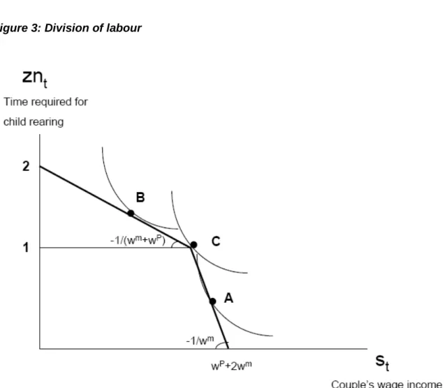
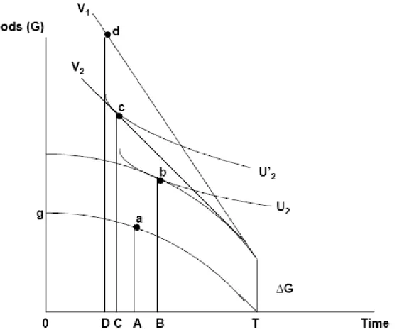
Figure 3 shows how utility and budget determine how many children a couple decides to have.

The optimal allocation of time for child rearing and savings (present value of future consumption) leads to three possible types of choices on the budget line (three intersections between the budged line and the utility curves).

When the optimal allocation is achieved at znt〈1, say at point A on the budget line, this leads to the decision that the woman works part-time and the man works full-time.

(33)

At point B, the woman does not participate in the labour market and performs child rearing full-time and the man contributes to child rearing part-time.

At point C, the parents share child rearing and labour market participation equally.

Hence, the time required for raising one child, z, and the utility of a child determines the desired number of children, n_t.

Figure 3: Division of labour

Source: Galor and Weil (1996)

The total time allocated to child rearing results from maximising the utility function (4.5), which is subject to (4.6) and (4.7):

(

)

[

m

]

t p t t w w zn =

γ

2+ / when

γ

[

2+

(

w_tp /w_tm

)

]

≤1

γ

2 = t zn when 2

γ

>1 1 = t zn otherwise (4.8)

(34)

This shows that women spend min

( )

1,2

γ

of their time raising children.

Case 1 implies that a higher percentage of women enter the job market when wage w_tm rises.

Figure 4 shows the effect of a shift of the budget line caused by a wage increase w_tm in point B.

Figure 4: Budget increase

Source: Galor and Weil (1996)

A reduction in the number of children gives the woman time for wage employment. The additional income provides more savings for the second period of life.

Case 2 implies for y>0,5 that women do not work independent of the wage level. However, it is empirically proved that the wage level influences a woman’s decision to work. This is why the restrictiony<0,5 is introduced and it reads:

Women's labour market participation interacting with macroeconomic growth and family policies

HAL Id: tel-00638278

https://tel.archives-ouvertes.fr/tel-00638278