HAL Id: hal-02285483
https://hal.archives-ouvertes.fr/hal-02285483
Submitted on 12 Sep 2019
HAL is a multi-disciplinary open access
archive for the deposit and dissemination of
sci-entific research documents, whether they are
pub-lished or not. The documents may come from
teaching and research institutions in France or
abroad, or from public or private research centers.
L’archive ouverte pluridisciplinaire HAL, est
destinée au dépôt et à la diffusion de documents
scientifiques de niveau recherche, publiés ou non,
émanant des établissements d’enseignement et de
recherche français ou étrangers, des laboratoires
publics ou privés.
Non-Invasive Localization of Atrial Flutter Circuit using
Recurrence Quantification Analysis and Machine
Learning
Haziq Azman, Olivier Meste, Gabriel Latcu, Kushsairy Kadir
To cite this version:
Haziq Azman, Olivier Meste, Gabriel Latcu, Kushsairy Kadir. Non-Invasive Localization of Atrial
Flutter Circuit using Recurrence Quantification Analysis and Machine Learning. Computing in
Car-diology, Sep 2019, Singapore, Singapore. �hal-02285483�
Non-Invasive Localization of Atrial Flutter Circuit using Recurrence
Quantification Analysis and Machine Learning
Muhammad Haziq Kamarul Azman
1 2, Olivier Meste
1, Decebal G. Latcu
3, Kushsairy Kadir
21
Universit´e Cˆote d’Azur, CNRS, I3S, France
2Universiti Kuala Lumpur, Malaysia
3Centre Hospitalier Princesse Grace, Monaco
Abstract
Atrial flutter presents quasi-periodic atrial activity due to circular depolarization. Given the different structure of right and left atria, spatiotemporal variability should be different. This was analyzed using recurrence quan-tification analysis. Autocorrelation signals were estimated from the unthresholded recurrence plot, calculated with a properly processed ECG to remove variability related to external sources (noise, respiratory motion, T wave over-lap). Simple features were considered from the autocorre-lation that attempts to describe the atrial activity in terms of range of recurrence and periodicity. Linear classifica-tion using support vector machines and logistic regression both allowed good classification performance (max accu-racy 0.8 for both). Feature selection showed that right and left AFL have significantly different cycle lengths (right vs. left:230.63 ms vs. 206.50 ms, p < 0.01).
1.
Introduction
The quasi-periodic atrial activity (AA) observed on the electrocardiogram (ECG) during atrial flutter (AFL) is caused by a rotating circular depolarization of the atrium. It has been shown that beat-to-beat variability of the flutter or F waves, quantified using vectorcardiographic parame-ters, allowed localization of right or left atrial circuit [1]. Different variability was observed for right and left local-ization, inducing a hypothesis of varying circuit stability.
With a beat-to-beat approach, instantaneous spatiotem-poral information is not preserved, which may contain in-formation about AA. In addition, both atria are known to be remarkably different in structure. The right atrium con-tains many large and well-defined cardiac fibers and is rel-atively thin, whereas the left atrium is thick and multi-layered [2]. It is expected that spatiotemporal variability would be different.
The use of recurrence quantification analysis (RQA) has been highlighted for spatiotemporal analysis and
charac-terization of atrial fibrillation (AF) activation propagation [3, 4]. Of particular interest, atrial fibrillation recurrence behavior was characterized, and was shown to be different for recurring and non-recurring persistent AF.
In this paper, RQA is employed in order to study the spatiotemporal variability related to the circular propaga-tion of AFL activapropaga-tion in a non-invasive fashion. Several features are extracted from the computed recurrence signal and serves as features for classification of circuit localiza-tion. Machine learning techniques are considered in order to obtain practical classifiers as well as to understand the reason why right and left AFL are different by employing feature selection.
2.
Methodology
2.1.
Dataset and Preprocessing
54 ECG recordings of AFL were used, acquired using a device (Boston Scientific, USA) at fs = 2000Hz, during
catheter ablation operation at Centre Hospitalier Princesse Grace, Monaco. A finite-impulse response notch filter at 50Hz was applied to these signals to remove powerline in-terference, as well as high- and low-pass filters to keep the band between [0.5; 70]Hz. Records with missing leads, low F wave amplitudes, low atrioventricular block ratio (< 2 : 1) and low F wave counts were excluded from the study. In total, there were 30 recordings with right circuit localization and 24 with left localization.
Extraction of atrial activity is crucial for RQA. However, in AFL the high synchronicity between atrial and ventricu-lar activity renders most extraction methods inefficient due to spectral overlap or source dependence. Segmentation of each F waves is preferred as an alternative to extract atrial activity. Since the essential activity is located fully within the F wave duration, the remaining portion of signals are theoretically not needed.
F waves from each recording were detected using a method developed previously [5]. Two set of F waves,
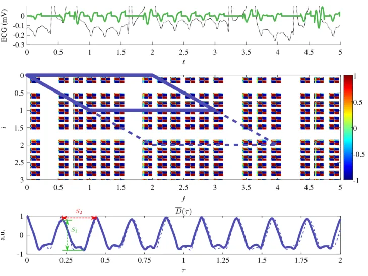
overlapped and not overlapped with T waves, were seg-mented. All F waves were synchronized, transformed into VCG and removed of respiratory motion using a technique described previously [1]. Overlapped F waves were cor-rected using the procedure detailed in a previous study [6]. The mean of each segmented F waves are removed for all leads. Finally, a new signal, different that the original recording, was made by replacing each wave at the same time index where it was originally located. The rest of the signal not containing any F waves are padded with zeros. This new signal represents the atrial signal free from any external variability (see 1, top panel).
2.2.
Calculation of Recurrence Features
Recurrence quantification analysis (RQA) is a non-linear technique that aims to quantify the properties of a dynamic, often oscillatory system by comparison of a state space vector x(i) of dimension K at one instant with an-other delayed instant x(i − τ ). In ECG analysis K rep-resents the number of leads available, and x(i) the ECG voltage at the discrete sample i . The state vector is then the multidimensional atrial dipole, and the ECG traces, the trajectory map of the dipole. Due to the circular depolar-ization, the trajectory resembles a loop.
The unthresholded recurrence plot (URP) R is a sym-metric 2D graphical plot representing a similarity measure D of two states at different delay instants, with the mea-sure being real-valued. This is written as:
R(i, j) = D(x(i), x(j)) (1)
One intuitive similarity measure that capture spatiotem-poral propagation of AA is the normalized dot product:
D(x(i), x(j)) = x(i)
Tx(j)
kx(i)kkx(j)k (2)
which is related to the cosine of the angle between the two vectors. This definition of recurrence captures not only the similarity of two very close state vectors, but it also captures similarity when the two vectors are in opposing directions. This was used successfully in the case of AF to characterize its spatiotemporal behavior [3].
A sample URP can be seen in 1 (middle panel) calcu-lated from a 5-second sample of the post-processed AFL signal(top panel). Due to the zero-padding of the post-processed signal, the URP contains many undefined recur-rence values (white area). When defined, the entries in the main diagonal are always 1, suggesting perfect match. Moving outwards from the main diagonal, repetitive pat-terns can be observed in intervals.
To limit non-stationarity, the URP was processed in seg-ments of fixed size. A segment starts at the main diagonal, and progresses along the diagonal up to a length I. The
segment width spans from the main diagonal towards the edge of the plot (i.e. increasing j) for up to a width J . The delay variable can be introduced by τ = j −i ⇔ j = i+τ . A segment can be described by the equation:
Rs(i, τ ) = R(i, i + τ ), i ∈ [(s − 1)I; sI] (3)
Highlights of segments can be found in Figure 1. The choice of I and J determines the properties of the segment, and should be considered as parameters. However, it can be reasoned in the context of AFL, that stationarity can be guaranteed for long periods of time due to the regularity of F wave manifestation. For this paper, I is set to 2000 samples (1 second), and J to 4000 samples (2 seconds). Note that τ ∈ [0; J ]. The value of J assures that > 5 AFL cycles can be captured in the segment.
To reduce the variance of the recurrence estimate, an average can be taken for each segment along i:
Ds(τ ) = 1 I sI X i=(s−1)I Ds(i, τ ) (4)
This amounts to an autocorrelation, assuming stationar-ity within the segment. In practive, undefined recurrence values were discarded, and for each τ , the average only considers defined values (i.e. I is not fixed), to avoid bias in the calculation. An example of this is shown in Figure 1 (bottom panels). It is clear that AFL has a quasi-periodic recurrence behaviour, as shown by the high and repetitive autocorrelation peaks.
To quantify this behavior, two parameters were consid-ered. The first parameter S1 relates to the range of
spa-tial propagation. This is given by the peak-to-peak ampli-tude of the autocorrelation, taken from one maximum to the next minimum (Figure 1, bottom panel, in green). The second parameter S2relates to the periodicity of
propaga-tion, and is essentially an estimate to the AFL cycle length. This is calculated by the peak-to-peak interval of the avail-able maximums. The two parameters are calculated for all available points in the signal, hence making a series of val-ues.
Calculation of these parameters can be done for each segment. However, the existence of long periods of unde-fined values can be troublesome, since long segments of discontinuity is present. In order to combat this problem, the autocorrelations were aggregated by calculating their median value:
˜
D = medianSs=1Ds (5)
The result is a single continuous autocorrelation func-tion. In some patients, the function ˜D was unfortunately still discontinuous due to prolonged undefined periods. This did not hinder the calculation of the parameters, though.
ECG (mV) i a.u. τ t j 1 -1 0.5 1.5 2 2.5 3 3.5 4 4.5 5 0.25 0.75 1.25 1.75 0 1 0.5 1.5 2 2.5 3 3.5 4 4.5 5 0 -0.1 0 -0.2 -0.3 1 0.5 1.5 2.5 2 3 0 1 0.5 0 -0.5 1 0 -1 0 0.5 1 1.5 2 S2 S1 D(τ )
Figure 1. Top panel: 5-second sample ECG (lead V1). Thin broken line indicates the post-filtered ECG, whereas thick
green line indicates the ECG after all processing steps. Middle panel: unthresholded recurrence plot calculated from the new ECG. Bottom panel: autocorrelation functions derived from their respective plots by averaging of single segments. First segment is shown (thick line) along with the subsequent segment (thin broken line). See Section 2.2 for details.
From the two parameters, several features were cal-culated, that aim to capture spatiotemporal variability in AFL: the 1) mean, 2) standard deviation, 3) variance, 4) skewness, and 5) kurtosis of the two series. The features are in fact statistical moments, and characterizes the prop-erties of the series distribution. In total, there were 10 fea-tures considered.
2.3.
Learning Protocol
The set of data and features were used as learning inputs to the linear support vector machine (SVM) and logistic re-gression (LOG) classifiers. Due to the small sample size, no validation schemes were considered. In order to eval-uate the relevance of the feature, a wrapper approach was employed by evaluating all possible combinations of
fea-tures from 1 to 10. Relevance of the feature was deter-mined by counting the participation of each feature in the combinations that produced the highest accuracy, from a combination length of 1 to 10, and summing the participa-tion score.
3.
Results and Discussion
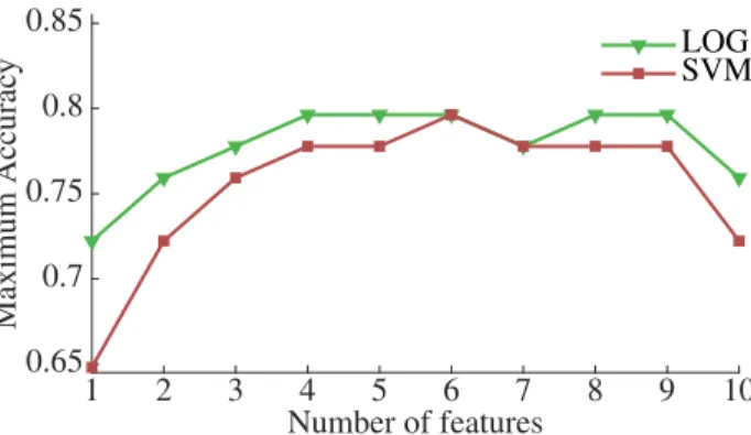
The result of classification is shown in Figure 2. As can be seen, recurrence quantification gave features that are discriminating with respect to AFL localization. Good performance can be achieved, as seen by accuracies > 0.6, and increases as more features are added. Maximum per-formance was obtained by all classifiers at 6 combinations of features (accuracy = 0.8, sensitivity and specificity = (0.67, 0.90) and (0.90, 0.67) for LOG and SVM
classi-1 2 3 4 5 6 7 8 9 10 Number of features 0.65 0.7 0.75 0.8 0.85 Maximum Accurac y SVMLOG
Figure 2. Maximum classifier accuracy of the considered classifiers.
fier respectively). This was obtained using linear clas-sifiers and with a small amount of features, suggesting that overfitting was avoided. The 6 features used were [F1F2F3F6 F7F9] for LOG, and [F1F2F5F6F7F9]
for SVM (refer to Table 1 for feature indices).
Table 1. Feature Scores
Index Feature LOG SVM
F1 Mean(S1) 8 6 F2 Stdev(S1) 7 7 F3 Var(S1) 7 8 F4 Skewness(S1) 4 1 F5 Kurtosis(S1) 4 7 F6 Mean(S2) 10 10 F7 Stdev(S2) 7 6 F8 Var(S2) 5 5 F9 Skewness(S2) 7 9 F10 Kurtosis(S2) 4 6
Further analysis of the relevant features was performed by counting the score of each feature: if the feature was involved in any combinations of length l that produced the maximum accuracy, then it is assigned a score of 1, else 0. The total score is the sum of scores from combination length 1 to 10. The largest possible score is then 10, and lowest 0.
Table 1 shows the feature score for each classifier. The highest participation was found to be of the feature F6.
This suggests that this feature presents a significant con-tribution in determining right or left localization. Interpre-tation of the feature indicates that right flutter have sig-nificantly larger cycle lengths (mean 230.63 ms) than left flutter (mean 206.50 ms; p < 0.01, Mann-Whitney U test). However, this does not conclude on whether if AA propa-gation was faster in left AFL or that the circuit was larger. Further investigation is required to clarify this matter.
4.
Conclusion
It has been shown that the ensemble of processing steps were able to extract meaningful characteristic parameters of the AFL AA propagation, and allowed localization to be performed with a good degree of performance. Recur-rence quantification analysis allowed access to spatiotem-poral characteristics of AFL, which was shown to be differ-ent for each localization. Inspection of the features showed that different AFL localization produced significantly dif-ferent propagation cycle lengths.
References
[1] Kamarul Azman MH, Meste O, Kadir K, Latcu DG. Local-izing atrial flutter circuit using variability in the vectorcar-diographic loop parameters. In Computing in Cardiology, volume 45. 2018; 4.
[2] Wang K, Ho SY, Gibson DG, Anderson RH. Architecture of atrial musculature in humans. Heart June 1995;73(6):559– 565.
[3] Meste O, Zeemering S, Lankveld T, Schotten U, Crijns H, Peeters R, Bonizzi P. Noninvasive recurrence quantification analysis predicts atrial fibrillation recurrence in persistent pa-tients undergoing electrical cardioversion. In Computing in Cardiology, volume 43. 2016; 677–680.
[4] Bonizzi P, Zeemering S, Karel J, Azman MH, Lankveld T, Schotten U, Crijns H, Peeters R, Meste O. Noninvasive char-acterisation of short-and long-term recurrence of atrial sig-nals during persistent atrial fibrillation. In Computing in Car-diology, volume 44. 2017; .
[5] Kamarul Azman MH, Meste O, Kadir K. Detecting flutter waves in the electrocardiogram using generalized likelihood ratio test. In Computing in Cardiology, volume 45. sep 2018; 4.
[6] Kamarul Azman MH, Meste O, Kadir K, Latcu DG. Estima-tion and removal of t wave component in atrial flutter ecg to aid non-invasive localization of ectopic source. In Comput-ing in Cardiology, volume 44. 2017; 4.
Address for correspondence: Muhammad Haziq Kamarul Azman Room 416
Universiti Kuala Lumpur, British Malaysian Institute Batu 8, Jalan Sungai Pusu
53100 Selangor, Malaysia [email protected]