HAL Id: hal-02613235
https://hal.archives-ouvertes.fr/hal-02613235
Submitted on 19 May 2020HAL is a multi-disciplinary open access archive for the deposit and dissemination of sci-entific research documents, whether they are pub-lished or not. The documents may come from teaching and research institutions in France or abroad, or from public or private research centers.
L’archive ouverte pluridisciplinaire HAL, est destinée au dépôt et à la diffusion de documents scientifiques de niveau recherche, publiés ou non, émanant des établissements d’enseignement et de recherche français ou étrangers, des laboratoires publics ou privés.
Extended Iwan-Iai (3DXii) constitutive model for
1-Directional 3-Component seismic waves in liquefiable
soils: application to the Kushiro site (Japan)-3C seismic
wave propagation in liquefiable soils
Maria Paola Santisi d’Avila, Viet Pham, Luca Lenti, Jean-François Semblat
To cite this version:
Maria Paola Santisi d’Avila, Viet Pham, Luca Lenti, Jean-François Semblat. Extended Iwan-Iai (3DXii) constitutive model for 1-Directional 3-Component seismic waves in liquefiable soils: applica-tion to the Kushiro site (Japan)-3C seismic wave propagaapplica-tion in liquefiable soils. Geophysical Journal International, Oxford University Press (OUP), In press. �hal-02613235�
Extended Iwan-Iai (3DXii) constitutive model for 1-Directional 3-Component
seismic waves in liquefiable soils: application to the Kushiro site (Japan)
Maria Paola Santisi d’Avila1
, Viet Anh Pham2, Luca Lenti3, Jean-François Semblat4
1Université Côte d’Azur, CNRS, LJAD, 06108 Nice, France. Email: msantisi@unice.fr 2
National University of Civil Engineering, Soil Mechanics and Foundation Engineering Division, Ha Noi, Viet Nam.
3
IFSTTAR, Université Paris-Est, 77447 Champs sur Marne, France.
4
ENSTA, IMSIA, 91761 Palaiseau, France.
Accepted date. Received date; in original form date
Abbreviated title: 1D-3C seismic wave propagation in liquefiable soils
Corresponding author: Maria Paola Santisi d’Avila Université Côte d’Azur - LJAD
28, Avenue Valrose - 06108 Nice - France Email: msantisi@unice.fr
SUMMARY
The influence of pore water pressure has to be taken into account when the propagation of seismic waves in saturated soils is simulated, because it controls the strength decrease during the dynamic process and can induce phenomena such as cyclic mobility and liquefaction. The decrease of effective stresses leads to permanent deformation in the soil and damages to the surface structures.
This research aims at validating a 1-Directional propagation model of 3-Component seismic waves (1D-3C) in a horizontally layered soil, in the case of saturated soil.
A three-dimensional nonlinear elasto-plastic model for soils is used and the variation of the shear modulus reduction curve with the pore water pressure is taken into account during the seismic event. In the case of multiaxial stress states induced by a 3C seismic motion, if no additional information is available, the modulus reduction curves in shear and compression, normalized with respect to the elastic moduli, are assumed identical, since the Poisson’s ratio is supposed to be constant during the process. The multiaxial stress state in saturated soils induced by a 3C seismic motion is analyzed for various stress paths.
The 1D-3C wave propagation model is used to compute the seismic response of the Kushiro soil profile (Japan). The stratigraphy and geotechnical properties are deduced from in-situ and laboratory tests provided by the PRENOLIN benchmark. Numerical results are in correct agreement with the records at the surface in terms of acceleration envelope.
Key words: saturated soil; effective stress; site effects; seismic wave propagation; nonlinear soil
1 INTRODUCTION
The development of excess pore water pressure in saturated soils when subjected to dynamic loading reduces the effective stress and can cause cyclic mobility and soil liquefaction (Kramer 1996).
This research aims at modeling the influence of the three-components (3C) of the seismic excitation taking into account the water table position and the nonlinear hysteretic behavior of saturated soil under cyclic loading.
Iwan’s elasto-plastic model (Iwan 1967; Joyner 1975; Joyner & Chen 1975) is adopted to
represent the three-dimensional (3D) nonlinear behavior of soil in the case of total stress analysis. Its main feature is the proper reproduction of nonlinear and hysteretic behavior of soils under cyclic loadings, with a minimal number of parameters characterizing the soil properties. A correction to the shear modulus, proposed by Iai et al. (1990a,b) for one-component (1C) shear loading, is used for saturated cohesionless soil layers to account for pore pressure build-up. Bonilla et al. (2005) used Iwan’s hysteretic model for two-dimensional analyses, in a finite difference formulation, combined with Iai’s liquefaction front model which considers the cyclic mobility and dilatancy of sands.
In this research, the implementation of the Iwan-Iai constitutive behavior model is firstly validated in the case of 1C shear stress, by comparison with Ishihara’s tests (Ishihara 1985) for dense and loose sand samples. Then, the Iai’s shear modulus correction for saturated soils is extended to multiaxial stress states induced by a 3C excitation. In Section 2, the constitutive behavior is shown for various stress paths in the case of dense and loose sands.
The proposed 3D Iwan-Iai constitutive model for saturated soil is adopted in a finite element scheme to simulate the vertical propagation of 3C seismic waves in a horizontally layered soil
basin (Section 3). The finite element model (FEM) used in this research is implemented in SWAP_3C code (Santisi et al. 2012, 2013; Santisi & Semblat 2014) that has been verified and validated during the PRENOLIN benchmark (Regnier et al. 2016) in the case of total stress analysis for nonlinear soil. PRENOLIN is an international benchmark targeted to one-dimensional nonlinear site response analysis where 23 different codes have been assessed with respect to actual measurements on real sites. The results presented by Regnier et al. (2018) concern the total stress analyses undertaken during the benchmark.
In this research, the extended 3D Iwan-Iai constitutive model for saturated soil is implemented in the FEM (SWAP_3C code) and used to reproduce the numerical simulations proposed during the PRENOLIN benchmark for a saturated soil profile in Japan, taking into account the pore water pressure.
The KSRH10 site (in Hokkaido region, Japan), which is instrumented by the Japanese strong motion network KIK-Net, has been selected for the present analysis, because it involves downhole as well as surface accelerometers. It has also been chosen in the PRENOLIN benchmark as a site where the assumption of vertical propagation and horizontally layered soil is reliable. The stratigraphy and geotechnical parameters of the KSRH10 soil profile are identified based on borehole investigations and laboratory tests requested by the PRENOLIN benchmark. Liquefaction front parameters are calibrated using the available cyclic consolidated undrained triaxial (CTX) tests. In Section 4, the simulation of the seismic response of KSRH10 soil profile to various events is validated in terms of ground motion at the surface, by comparison with records. Profiles of maximum stress, strain, excess pore water pressure and soil motion with respect to depth are also estimated. The conclusions are discussed in Section 5.
2 NONLINEAR CONSTITUTIVE MODEL FOR 3-COMPONENT EXCITATION
The Iwan hysteretic model is adopted in the present analyses, in the case of 3D stress state induced by a 3C seismic loading, combined with the Iai’s correction that leads to consider the cyclic mobility and dilatancy of sands.
2.1 Nonlinear dry soil behavior
The 3D elasto-plastic soil model used in this research is implemented in a finite element scheme, according to that suggested by Iwan (1967), Joyner (1975) and Joyner and Chen (1975) in a finite difference formulation, in terms of total stresses.
According to Joyner (1975), the tangent constitutive matrix is deduced from the actual strain level and the strain and stress values at the previous time step. Then, the knowledge of this matrix allows calculating the stress increment. Consequently, the stress level depends on the strain increment and strain history but not on the strain rate. Therefore, this rheological model has no viscous damping. The energy dissipation process is purely hysteretic and does not depend on the frequency.
Iwan’s model is a 3D elasto-plastic model with linear kinematic hardening that allows taking
into account the nonlinear hysteretic behavior of soils. The model is calibrated using the elastic moduli in shear and compression and the shear modulus reduction curve is employed to deduce the size of the yield surface.
The elastic parameters given as input data are the shear modulus G0 vs2 (where is the mass
density and vs the shear wave velocity in the medium) and the P-wave modulus M0 v2p
(where vp is the pressure wave velocity in the medium).
behavior. This assumption is acceptable for soils in undrained conditions, as during an earthquake. However, Iai’s correction for effective stress analysis is pressure-dependent. The plasticity model assumes an associated plastic flow, which allows for isotropic yielding.
The backbone curve τ γ
G
γ , where G
is the shear modulus reduction curve with respect to shear strain , is needed to characterize the nonlinear soil behavior. The main feature of Iwan’s model is that the mechanical parameters to calibrate the rheological model can beobtained from laboratory dynamic tests on soil samples.
In the present study, the normalized shear modulus reduction curves provided by laboratory tests
are fitted by the function G
G01 1
r0
, where r0 is a reference shear straincorresponding to an actual tangent shear modulus G
equivalent to 50% of the elastic shear modulus G0. This model provides a hyperbolic stress-strain curve (Hardin & Drnevich 1972),having an asymptotic shear stress of 0 G0r0 in the case of simple shear.
2.2 Extension of liquefaction front model to a 3-Component stress path
A correction to the G G0 curve, proposed by Iai et al. (1990a,b) in the case of 1C shear loading,
is adopted for saturated soils and effective stress analysis. Iai’s rheological model for saturated soils allows to reach larger strains with proper accuracy.
In this research, the same correction procedure is adopted in the case of 3C excitation (two shear components and an axial component). If no additional information is available, the normalized compressional modulus reduction curve E E0 is assumed equal to the shear modulus reduction
curve G G0, under the commonly agreed hypothesis of constant Poisson’s ratio during the time
2 1E G .
Note that in the proposed formulation the prime indicates effective stresses. According to Terzaghi’s law, the average effective stress is defined as p
1 2 3
3 p u, where
1 2 3
3p is the average total stress, 1, 2 and 3 are the principal stresses and u is
the pore water pressure. The initial average effective stress is p0. The deviatoric stress is
max min
2 , where max and min are the maximum and minimum principal stresses,
respectively.
The liquefaction front (Iai et al. 1990a,b) in the
r S plane is represented in Fig. 1, where ,0
S p p is the state variable, with 0 S 1, and r p0 is the deviatoric stress ratio. The
state variable S relates the initial and the actual average effective stress and it is expressed as
0 3 2 2 2 0 2 3 1 3 S r r S S S S r r m r r (1)a,bwhere m1tan sin is the failure line slope (Fig. 1) and is the shear friction angle. It can be remarked in Fig. 1 that
r2r3
S0S2
m1. Accordingly, the parameter S2 is obtained as
2 0 2 3 1
S S r r m (2)
In equation (2), r2 m S2 0, r3 m S3 0, m3 0.67m2 and m2 tan p sinp is the phase transition line slope (Fig. 1), where p is the phase transformation angle. The initial value of liquefaction front parameter S0 is determined by imposing the initial condition S1 in equation
(1)b, according to (2). In dry and non-liquefiable layers, it is S1 during the seismic event. Iai et al. (1990a,b) provide a relationship to correlate the liquefaction front parameter S0 and the
normalized shear work w, as follows:
2 1 0 1 1 1 1 0 1 1 1 0.4 1 0.6 , 1 p p S S w w S w w S w w w w S (3)a,b Accordingly, it is
2 1 1 1 0 1 1 0 1 1 0 0 0.4 0.4 1 0.6 0.4 p p w w S S S S w w S S (4)a,bThe normalized shear work is wW Ws n . The normalization factor is Wn
p m0 1
r0 2, where r0 is the reference strain used in the hyperbolic formulation adopted for the backbone curve. The plastic shear work Ws is unknown for the initial state and it is estimated from w,according to equation (4), and Wn. The correlation between S0 and w, in equation (4), depends
on four material parameters S1, w1, p1 and p2 that characterize the liquefaction properties of the
cohesionless soil.
The main process starts with the computation of the actual plastic shear work. The increment of plastic shear work at each time step is
1
0s st se
dW R dW c dW (5)a,b
where, according to Towhata and Ishihara (1985), the shear stress work dWst is evaluated as the
difference between the total work dW ijd ij and the consolidation work dWc p d v, where v
d is the volumetric strain increment. There is an amplitude threshold for the cyclic shear strain or shear stress. There is no pore water pressure build-up for cyclic strain or stress below this threshold. The shear work spent over the threshold is subtracted from the total shear work. It is
correct the elastic shear work dWse for the purpose of obtaining the shear work spent over the
threshold. R is a correction factor for dWs in the case of dilatancy
p m0 2
and r S m3. Itis defined as
1 1 3 0 1 1 3 0 0.4 0.4 0.4 R m r m m S R m r S m m S (6)a,bWhen the actual plastic shear work Ws is known, the normalized shear work w is evaluated, the
liquefaction front parameter S0 is deduced from equation (3) and the state variable S is obtained
by equation (1). According to the definition of S , the actual average effective stress pS p0
and the increment of water pressure u p0 p0 are obtained during the time history. The actual effective stress u is deduced from the total stress and water pressure u p p. Finally, the updated deviatoric stress a and the reference shear strain ra are estimated as
0 0 0 0 0 0 1 2 0 0 0 0 0.4 1 0.4 0.4 0.4 a ra r a ra r S S S S m m S S S (7)a,bThe corrected shear modulus is
a a ra
G (8)a,b
Consequently, the normalized shear modulus reduction curve is updated as
a 1 1
ra
G G .
2.3 Calibration of saturated soil parameters
Iai’s correction of shear modulus for saturated soils needs the knowledge of the shear friction
corrects the elastic shear work, and S1, w1, p1 and p2 that influence the relationship between the
liquefaction front parameter S0 and the normalized shear work w.
A Consolidated Undrained (CU) triaxial test provides the shear friction angle and the phase transformation angle p, using a
, p
curve for three different confining pressure levels. Theslope of the line connecting the rupture points, for the three different confining pressure levels, is the trigonometric tangent of angle . The slope of the line connecting the inflection points of
the three curves is the trigonometric tangent of angle p. The shear friction angle and the
phase transformation angle p are obtained considering the equivalences tan sin and
tan p sinp, respectively.
According to Iai et al. (1990a,b), the liquefaction front parameters S1, w1, p1 and p2 are
calibrated by a trial-and-error procedure to best reproduce the curves obtained by CTX tests. The cyclic deviatoric stress generated during the test (axial stress minus confining pressure) is adopted as the input in a numerical simulation. Two curves have to be obtained numerically and compared to the curves produced during the test: the deviatoric strain amplitude and the normalized excess pore water pressure u p0 with respect to the number of loading cycles N , where u p0 p is the excess pore water pressure. The initial effective confining pressure during the test is p0 p0 u0, where p0 is the cell pressure and u0 is the back pressure.
In order to obtain numerically the curves that best reproduce the experimental ones, the parameters w1 and p1 are determined by a trial-and-error procedure, to obtain a normalized
excess pore water pressure curve that best reproduce the portion of the experimental curve for
0 0.6
u p
determined at first for a given value of p1. The appropriate value of p1 is researched in the
interval
0.4 0.7
, according to Iai et al. (1990b). The greater w1 and p1, the lower the excess pore water pressure. The envelope of strain amplitude is also fitted, observing that the greater1
w , the lower the envelope of strain amplitude.
The parameter p2 is searched in the interval
0.6 1.5
(Iai et al. 1990b). It is determined as well by a trial-and-error process, to obtain a normalized excess pore water pressure curve that best fit the portion of the experimental curve for u p0 0.6. Since the curve is not greatly influenced by the variation of p2, the envelope of strain amplitude is also fitted. The greater p2, the largerthe envelope of strain amplitude.
Parameter S10.005 is introduced so that S0 will never be zero. It takes small positive values,
determined by the trial-and-error procedure to obtain the best fit of the experimental normalized excess pore water pressure curve.
According to Iai et al. (1990b), parameter c1 is imposed equal to one when w1, p1 and p2 are
determined and, if laboratory data are not well represented in the elastic range, c1 can be
modified using a trial-and-error procedure.
2.4 Three-component vs one-component loading
Ishihara’s tests (Ishihara 1985) for dense and loose sands are reproduced according to Iai’s
model (Iai et al. 1990a,b). The geotechnical parameters of the analyzed soil samples are listed in
Table 1. The initial average effective stress in the tests is p0 98 kN m2 . Numerical curves are compared with experimental results in Figures 2 and 3, respectively. In this way, the implementation of the constitutive model is validated.
The zx shear stress loading of Ishihara’s tests (Ishihara 1985) is numerically imposed to dense and loose sand samples in the case of a 3C stress loading. A yz shear stress equal to the halved
zx shear stress is imposed to induce higher strains compared with the case of two equivalent shear components. A 3C loading condition is analyzed, where a zz axial stress equal to one fourth of the zx shear stress is given. The response of the dense and loose sand samples is shown in Figs 4 and 5, respectively. The dense sand is less influenced by the 3C loading than the loose sand, where the shear strain is higher for 3C loading and the excess pore water pressure increases for a reduced number of cycles. In both cases, the maximum deviatoric stress ratio increases for 3C-loading, compared with a 1C shear loading.
Another case is analyzed where the zz axial stress has amplitude equal to the zx shear stress applied in Ishihara’s tests. A yz shear stress equal to the halved zx shear stress is imposed. The
response of the dense and loose sand samples is shown in Figs 6 and 7, respectively. The dense sand shows reduced axial strain in the case of 3C loading, a light increase of excess pore water pressure in the first cycles and an increased deviatoric stress ratio. The 3C loading in loose sand increases the axial strain, increases the excess pore water pressure for a reduced number of cycles and increases the deviatoric stress ratio, compared with a 1C shear loading.
3 1D-3C WAVE PROPAGATION IN SATURATED SOIL
The numerical simulation of the vertical propagation of 3C seismic waves along a horizontally layered soil is undertaken using a finite element model. The multilayered soil (Fig. 8) is assumed infinitely extended along the horizontal directions x and y and, consequently, no
strain variation is considered in these directions. A 3C seismic wave propagates vertically in the
behavior.
The soil profile is discretized into quadratic line finite elements having three translational degrees of freedom per node. The finite element model applied in the present research is completely described in Santisi d’Avila et al. (2012).
As the considered horizontally layered system is bounded at the top by the free surface, the stresses normal to the free surface are assumed to be null. At the bottom, a downhole motion in terms of acceleration can be imposed at the first node (Santisi d’Avila & Semblat 2014), containing incident and reflected waves. Otherwise, a 3C incident motion in terms of velocity at the bedrock level can be imposed and the soil motion at the soil-bedrock interface (first node of the mesh in Fig. 8) is computed during the process using an absorbing boundary condition. On this topic, the interested reader can refer to Joyner & Chen (1975) and Santisi d’Avila et al. (2012) for more details.
The time integration of the equation of motion is performed through Newmark’s algorithm. The two parameters 0.3025 and 0.6 guarantee an unconditional numerical stability of the time integration scheme (Hughes 1987). Moreover, the nonlinearity of soil demands the linearization of the constitutive relationship within each time step. The discrete dynamic equilibrium equation does not require an iterative solving to correct the tangent stiffness matrix,
within each time step, if a small time step 4
10 s
dt is chosen.
4 NUMERICAL SEISMIC RESPONSE OF KSRH10 SOIL PROFILE
KSRH10 site is located in Kushiro (Hokkaido region, Japan). It is a deep sedimentary site with
39 m of low velocity soil layers and a downhole sensor located at a depth of 255m. More
The stratigraphy and the geotechnical parameters of the analyzed KSRH10 Japanese soil profile are presented in Table 2, directly given by the reports of borehole and laboratory tests requested during the PRENOLIN benchmark, without corrections. Shear wave velocity and Poisson’s ratio profiles with respect to depth are given using in-situ measures. The compressional wave velocity
p
v is deduced from these parameters as 2
22 1 1 2
p s
v v , where vs is the shear velocity and is the Poisson’s ratio. The total (wet) density is obtained by laboratory tests. Consequently, the elastic shear modulus is evaluated as 2
0 s
G v and the elastic P-wave modulus is evaluated as M0 v2p.
A series of CTX tests using different axial stress amplitudes are employed to obtain the
normalized reduction curve of the modulus in compression E
z E0CTX, where E0 CTX is theYoung modulus obtained during the CTX test for low values of strain. The related shear
modulus reduction curve G
G0CTX is obtained by imposing G G0 CTX equal to E E0 CTX andthe relationship
z 3
between the axial stress
z and the shear stress
. It means that E0CTX G0CTX
z 3
. This assumption implies a constant Poisson’s ratio during the seismic event. Laboratory tests (as a resonant column test to obtain the shear modulus reduction curve) are not available for the analyzed case study to confirm this hypothesis. Anyway, it has been accepted during the PRENOLIN benchmark to provide the shear modulusreduction curve based on E
z E0CTX curves.The normalized shear modulus reduction curve G
G0CTX is fitted using the curve
0CTX 1 1
r0
G G , corresponding to a hyperbolic stress-strain curve. The reference
considered linear behaving below 39 m.
A further correction of the normalized shear modulus reduction curve has been proposed during the PRENOLIN benchmark (Regnier et al. 2018), replacing the initial shear modulus G0 CTX,
obtained during the CTX test, by an assumed higher value. This correction is not applied in this study, because the variation of the seismic response of the soil column is not strongly affected by this assumption and, in this case, it does not ameliorate the numerical results significantly.
The shear friction angle and the phase transformation angle p are obtained from static CU
triaxial tests, measuring the failure and phase transition line slope tan and tanp,
respectively, in the plan
, p
, and considering the equivalences tan sin andtan p sinp. The obtained angles are reported in Table 2.
The liquefaction front parameters are reported in Table 2 for noncohesive soil layers, subjected to possible liquefaction phenomena. The calibration of liquefaction front parameters, from CTX test curves, is shown in Fig. 9 for the first layer. The analyzed test appears not sensitive to a variation of S1 and c1. The first trial is maintained for all the layers: S10.005 and c11. The
axial strain amplitude with respect to the number of loading cycles N obtained by CTX tests (Fig. 9) has been corrected by a 0.05Hz 4-pole non-causal Butterworth highpass filter to obtain a zero mean curve.
According to PRENOLIN benchmark reports, the measured water table depth in December 12th, 2013, is dw 2.4 m(Fig. 8) and this depth is used for the present analysis.
The variation of the elastic shear modulus with depth is taken into account for the liquefiable
soil layers. It is corrected according to G z0
G z0
m p z0 p z0 m , where p0 is the average effective pressure, zm is the depth at the middle of the layer and G z0
m vs2 is estimatedusing the values of density and shear velocity reported in Table 2 for the soil layer. In non-liquefiable layers, the shear modulus is assumed constant with depth.
The average effective stress in geostatic conditions p0
v 2 h
3 is evaluated considering the vertical effective stress v
z g z u z 0
, variable with depth z (where g is the gravitational acceleration) and dependent on the initial pore water pressure u0
z , and thehorizontal effective stresses estimated as h
z K0v
z . The at-rest lateral earth pressure coefficient is evaluated as K0
1
1 2v v2s 2p. At the surface, where the vertical stress reaches zero the horizontal effective stresses are corrected and assumed equal to h K0v
zpin the first zp meters (in this study, it is assumed zp 5 m). This setting is necessary firstly
because the horizontal stress is reduced but is not null at the surface and, secondly, because the shear modulus correction process depends on the actual to initial average effective stress ratio
0
p p and if p0 resulted null at the surface, the shear modulus would not be updated.
At the KSRH10 site, a set of input motions (Table 3) has been selected during the PRENOLIN benchmark to represent different borehole peak ground acceleration (PGA) and frequency content. According to Regnier et al. (2018), input signals have been processed removing the mean, applying a tapering Hanning window on 2% of the signal and non-causal filtering between 0.1 and 40 Hz. The three components of motion are recorded in North–South, East– West and Up–Down directions, respectively referred to as x, y and z in the present analysis.
4.1 Acceleration time histories at the surface
The numerical acceleration time histories are compared with records in Figs 10-12, separated in three groups according to the borehole peak acceleration (BPA) level (Table 3): BPA lower than
2
0.1m s ; BPA between 0.2 m s2 and 0.3 m s2; BPA higher than 0.6 m s2.
All numerical signals are filtered using a 4-pole non-causal Butterworth bandpass filter in the frequency range 0.1 10 Hz .
The computed acceleration time histories reproduce well the acceleration envelope in the horizontal directions. The vertical component is satisfactorily reproduced for the smaller events from TS-9 to TS-2 and it is too much amplified for strongest earthquakes TS-1 and TS-0.
Some parameters characterizing a signal are employed to quantitatively estimate the reliability of the obtained numerical signals, compared with seismic records. According to Anderson’s criteria (Anderson 2004), the Goodness-of-fit is represented using grades between 0 and 10, assigned to Arias duration (C1), energy duration (C2), peak acceleration (C5) and cross correlation ratio (C10). Scores in the intervals 0-4, 4-6, 6-8 and 8-10 represent poor, fair, good and excellent fit, respectively. The PGA for recorded and numerical signals at the surface of the KSRH10 soil profile are compared in Tables 4 and 5, for the horizontal motion in x- and y-direction, respectively, and the scores obtained according to Anderson criteria are listed.
The analyses in terms of total stresses, undertaken during the PRENOLIN benchmark, have shown that the adopted model overestimates the peak acceleration for small events, due to the fact that only hysteretic damping is considered during the process and no viscous damping. Consequently, the damping effect is too reduced for small strain levels. The same effect is obtained in the presented effective stress analyses (Figs 10 and 11, Tables 4 and 5).
According to Regnier et al. (2018), the frequency content is more difficult to reproduce correctly, for this site, over the whole frequency range. During the PRENOLIN benchmark, it has been underlined that the hypotheses of one-directional propagation in horizontally layered media might be violated in the analyzed site, even though it has been selected for the code
validation to minimize the impact of these assumptions. Probably, this site has a more complex geometry. However, more complex geometries require more detailed site characterization over a broader area, adequate interpretation of the data and computationally expensive 3D numerical simulations.
4.2 Seismic response at different depths
The profiles with depth of maximum shear stress, shear strain, horizontal motion and excess pore water pressure, computed numerically, are presented in Figs 13-15. These results show the different seismic response at each depth and the most impacted layers. It can be confirmed that the nonlinear soil behavior and the various frequency content of the seismic event yield a seismic response along the depth that is not directly proportional to the borehole peak acceleration.
5 CONCLUSIONS
A 3D nonlinear constitutive model for saturated soils is used in a 1-Directional propagation model of 3-Component seismic waves (1D-3C). The proposed model allows taking into account the input seismic wave polarization and the effect of pore water pressure, under the assumption of one-directional propagation in a horizontally layered soil.
The 3D behavior of saturated dense and loose sand is analyzed using an extended Iwan-Iai constitutive model, for different multiaxial stress states. The dense sand is less influenced by the 3C loading than the loose sand, where axial and shear strain appears higher for 3C loading and the excess pore water pressure increases for a reduced number of cycles. The maximum deviatoric stress ratio is higher for 3C loading, compared with a 1C shear loading.
The 1D-3C wave propagation model is used to numerically simulate the seismic response of the KSRH10 Japanese soil profile, by deducing the soil geotechnical properties by in-situ and laboratory tests provided by the PRENOLIN benchmark. Numerical signals reproduce satisfactorily the analyzed records at the surface in terms of acceleration envelope. The numerical simulations provides the profiles of maximum stress and strain, ground motion and excess pore water pressure with respect to depth.
Even though the KSRH10 soil profile has been selected because extensive site characterization has been performed, involving in-situ and laboratory measurements of the soil properties, this site seems to have complex geometry and the assumptions of one-directional propagation and horizontally layered soil might not be assured. For this site, the frequency content cannot be retrieved correctly over the whole frequency range, also using an effective stress analysis.
The commonly agreed hypothesis of constant Poisson’s ratio during an earthquake is applied
because laboratory tests are not available to provide both modulus reduction curves in shear and in compression, for the characterization of soil nonlinearity in the case of a 3C loading. Nevertheless, laboratory tests will be performed to study the relevance of this hypothesis.
Further work will be necessary to compare the obtained results with those of some other codes that have been validated during the PRENOLIN benchmark and that carry out effective stress analyses.
AKNOWLEDGMENTS
The first studies of the adopted constitutive model for liquefiable soils have been developed thanks to the PhD thesis of Viet Anh Pham, funded by IFSTTAR (Paris, France).
numerical simulations have been performed at the Laboratoire Jean Alexandre Dieudonné (Université de Nice Sophia Antipolis, Nice, France), thanks to its computer cluster.
This research has been possible thanks to the data detailed in the reports of laboratory and in-situ geotechnical tests provided by the PRENOLIN benchmark. The authors thanks Julie Regnier for her work during the PRENOLIN benchmark and for the help to remember the reflections that inspired the different iterative steps undertaken during the benchmark.
The authors thank Fabian Bonilla for having inspired, with his previous research, the selection of Iwan-Iai constitutive model for liquefiable sands and having collaborated with the organization team of PRENOLIN benchmark.
REFERENCES
Anderson, J.G., 2004. Quantitative measure of the goodness-of-fit of synthetic seismograms,
Proceedings of the 13th World Conference on Earthquake Engineering, Vancouver, Canada,
Paper No. 243.
Bonilla, L.F., Archuleta, R.J. & Lavallée, D., 2005. Hysteretic and dilatant behavior of cohesionless soils and their effects on nonlinear site response: field data observations and modeling, Bull. seism. Soc. Am., 95(6), 2373–2395.
Hardin, B.O. & Drnevich, V.P., 1972. Shear modulus and damping in soil: design equations and curves, J. Soil Mech. Found. Div., 98, 667–692.
Hughes, T.J.R., 1987. The finite element method - Linear static and dynamic finite element
analysis, Prentice Hall, Englewood Cliffs, New Jersey.
Iai., S., Matsunaga, Y. & Kameoka, T., 1990a. Parameter identification for a cyclic mobility mode, Report of the Port and harbour Research Institute, 29(4), 27–56.
Iai., S., Matsunaga, Y. & Kameoka, T., 1990b. Strain space plasticity model for cyclic mobility,
Report of the Port and harbour Research Institute, 29(4), 57–83.
Iwan, W.D., 1967. On a class of models for the yielding behavior of continuous and composite systems, J. Appl. Mech., 34, 612–617.
Ishihara, K., 1985. Stability of natural deposits during earthquakes, Proceedings of the 11th
International Conference on Soil Mechanics and Foundation Engineering, San Francisco, Vol.
1, pp. 327–376.
Joyner, W.B., 1975. A method for calculating nonlinear seismic response in two dimensions,
Bull. seism. Soc. Am., 65(5), 1337–1357.
Joyner, W.B. & Chen, A.T.F., 1975. Calculation of nonlinear ground response in earthquakes,
Bull. seism. Soc. Am., 65(5), 1315–1336.
Kramer, S.L., 1996. Geotechnical earthquake engineering, Prentice Hall, New York.
Régnier, J. et al., 2016. International benchmark on numerical simulations for 1D, nonlinear site response (PRENOLIN): Verification phase based on canonical cases. Bull. seism. Soc. Am., 106(5), 2112–2135.
Régnier, J. et al., 2018. PRENOLIN: international benchmark on 1D nonlinear site response analysis - Validation phase exercise. Bull. seism. Soc. Am., 108(2).
Santisi d’Avila, M.P., Lenti, L. & Semblat, J.F., 2012. Modeling strong seismic ground motion:
3D loading path vs wavefield polarization, Geophys. J. Int., 190, 1607–1624.
Santisi d’Avila, M.P., Semblat, J.F. & Lenti, L., 2013. Strong Ground Motion in the 2011
Tohoku Earthquake: a 1Directional - 3Component Modeling, Bull. seism. Soc. Am., Special issue on the 2011 Tohoku Earthquake, 103(2b), 1394–1410.
Santisi d’Avila, M.P. & Semblat, J.F., 2014. Nonlinear seismic response for the 2011 Tohoku
earthquake: borehole records versus one-directional three-component propagation models,
Geophys. J. Int., 197, 566–580.
Towhata, I. & Ishihara K., 1985. Shear work and pore water pressure in undrained shear. Soils
FIGURE LEGENDS
Figure 1. Liquefaction front r S , where
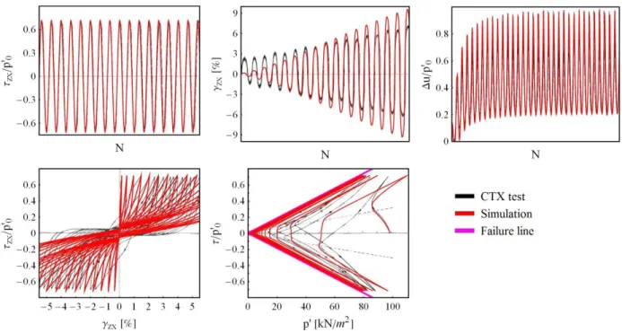
r is the deviatoric stress ratio and S is the state variable.Figure 2. Verification of the implemented soil constitutive model for saturated soil: fitting of
cyclic Consolidated Undrained triaxial test curves obtained by Ishihara (1985) for dense sand, using the calibration parameters proposed by Iai et al. (1990a,b).
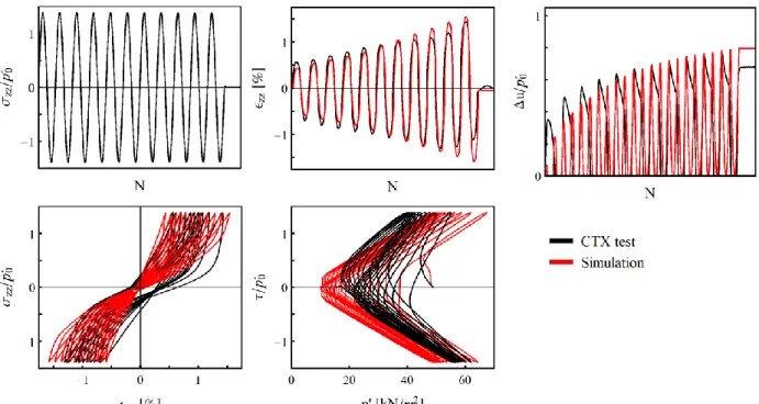
Figure 3. Verification of the implemented soil constitutive model for saturated soil: fitting of
cyclic Consolidated Undrained triaxial test curves obtained by Ishihara (1985) for loose sand, using the calibration parameters proposed by Iai et al. (1990a,b).
Figure 4. Strain and excess pore water pressure with respect to the number of cyclic loading
(top); shear stress-strain curve and deviatoric stress ratio with respect to the actual average effective pressure (bottom), in the case of dense sand for one-, two- and three-component loading.
Figure 5. Strain and excess pore water pressure with respect to the number of cyclic loading
(top); shear stress-strain curve and deviatoric stress ratio with respect to the actual average effective pressure (bottom), in the case of loose sand for one-, two- and three-component loading.
Figure 6. Strain and excess pore water pressure with respect to the number of cyclic loading
(top); shear stress-strain curve and deviatoric stress ratio with respect to the actual average effective pressure (bottom), in the case of dense sand for one-, two- and three-component loading.
Figure 7. Strain and excess pore water pressure with respect to the number of cyclic loading
effective pressure (bottom), in the case of loose sand for one-, two- and three-component loading.
Figure 8. Spatial discretization of a horizontally layered soil, loaded by a three-component
seismic motion applied at the soil-bedrock interface in terms of incident velocity, in the case of water table depth dw.
Figure 9. Fitting of cyclic Consolidated Undrained triaxial test curves to calibrate liquefaction
parameters for the soil layer 1 in KSRH10 soil profile, where the initial average effective
pressure in the test is p0 49 kN m2.
Figure 10. Recorded and numerical acceleration time history at the surface of the KSRH10 soil
profile for seismic events TS-7 (left), TS-8 (middle) and TS-9 (right).
Figure 11. Recorded and numerical acceleration time history at the surface of the KSRH10 soil
profile for seismic events TS-4 (left), TS-5 (middle) and TS-6 (right).
Figure 12. Recorded and numerical acceleration time history at the surface of the KSRH10 soil
profile for seismic events TS-0 (a, left) and TS-1 (a, right), TS-2 (b, left) and TS-3 (b, right).
Figure 13. Profiles with depth of maximum shear strain and stress, horizontal velocity and
acceleration in x-direction, for different seismic events, in KSRH10 soil column.
Figure 14. Profiles with depth of maximum shear strain and stress, horizontal velocity and
acceleration in y-direction, for different seismic events, in KSRH10 soil column.
Figure 15. Profiles with depth of maximum excess pore water pressure, for different seismic
TABLES Table 1.
Geotechnical parameters of soils samples used to validate the implementation of Iai’s model (Iai 1990a,b) in the case of one-component shear, by comparison with Ishihara’s tests (Ishihara 1985). The reference shear strain is estimated as r p m G0 1 0, where the initial average effective pressure in the test is 2
0 98 kN m
p .
Soil G0 M0 r m1 m2 S1 c1 p1 p2 w1
sample (kN/m2) (kN/m2) (‰) (rad) (rad)
Dense sand 140700 374247.7 0.6338 0.91 0.42 0.0050 1 0.45 0.72 2.85 Loose sand 103700 408766.7 0.8222 0.87 0.42 0.0035 1 0.45 1.40 2.00
Table 2.
Stratigraphy and mechanical features of KSRH10 soil profile
depthH255m
. Soil Depth Thickness vs vp r ’ p’ p1 p2 w1layer (m) (m) (kg/m3) (m/s) (m/s) (‰) (°) (°) 1 6.0 6.0 1760 140 1520 1.10 36.2 16.0 0.4 0.6 32 2 11.0 5.0 1820 180 1520 1.00 35.2 16.0 0.4 0.6 60 3 15.0 4.0 1480 230 1650 1.75 43.3 4 20.0 5.0 1480 300 1650 1.75 43.3 5 24.0 4.0 1580 250 1650 0.65 42.8 19.9 0.4 0.6 40 6 28.0 4.0 1580 370 1650 1.90 37.8 23.2 0.4 0.6 100 7 35.0 7.0 1800 270 1650 1.90 37.8 23.2 0.4 0.6 100 8 39.0 4.0 1800 460 1650 1.50 16.4 9 44.0 5.0 2510 750 3510 100 10 84.0 40.0 2510 1400 3510 100 11 255.0 171.0 2510 2400 5900 100
Table 3.
Input seismic motions used in the numerical simulations for KSRH10 soil profile.
Event Earthquake Magnitude Epicentral distance BPA PGA number code (Mw) (km) (m/s2) (m/s2) TS-0 KSRH10 0309260450 8.0 180 1.14 5.81 TS-1 KSRH10 0411290332 7.1 32 0.81 3.64 TS-2 KSRH10 0412062315 6.9 44 0.69 4.37 TS-3 KSRH10 0411290336 6.0 37 0.64 2.04 TS-4 KSRH10 0404120306 5.8 43 0.27 1.86 TS-5 KSRH10 0904282021 5.4 69 0.25 1.64 TS-6 KSRH10 0501182309 6.4 38 0.25 1.27 TS-7 KSRH10 0912280913 5.0 39 0.09 0.65 TS-8 KSRH10 0805110324 5.1 63 0.08 0.60 TS-9 KSRH10 0309291137 6.5 105 0.07 0.58 Table 4.
Comparison of recorded and numerical PGA at the surface of KSRH10 soil profile and scores obtained according to C1 (Arias duration), C2 (energy duration), C5 (peak acceleration) and C10 (cross correlation ratio) Anderson criteria, for the ground motion in x-direction.
Event Rec PGA Num PGA AI EI PGA CCr Number (m/s2) (m/s2) C1 C2 C5 C10 TS-0 5.34 5.15 7.9 8.5 10 4.2 TS-1 3.64 4.13 8.4 6.4 9.8 6.1 TS-2 3.35 3.48 7.2 6.4 10 7.4 TS-3 2.04 3.62 8.1 6.1 5.5 5.1 TS-4 1.86 2.76 8.9 6.4 7.9 5.6 TS-5 1.63 3.49 8.6 5.7 2.7 8.3 TS-6 1.23 2.04 7.4 4.8 6.5 4.9 TS-7 0.51 0.77 7.9 6.6 7.7 6.5 TS-8 0.33 0.99 8.7 5.6 0.2 7.6 TS-9 0.50 1.23 8.5 8.1 1.2 5.5
Table 5.
Comparison of recorded and numerical PGA at the surface of KSRH10 soil profile and scores obtained according to C1 (Arias duration), C2 (energy duration), C5 (peak acceleration) and C10 (cross correlation ratio) Anderson criteria, for the ground motion in y-direction.
Event Rec PGA Num PGA AI EI PGA CCr Number (m/s2) (m/s2) C1 C2 C5 C10 TS-0 5.81 7.32 7.5 7.9 9.3 3.9 TS-1 2.74 4.64 8.6 6.7 6.2 7.6 TS-2 4.37 7.45 4.8 5.5 6.1 6.9 TS-3 1.94 3.59 8.4 5.7 4.9 4.8 TS-4 1.39 4.60 9.2 7.9 0.0 2.6 TS-5 1.64 3.35 7.9 5.4 3.4 6.3 TS-6 1.27 3.44 8.7 5.5 0.5 4.4 TS-7 0.65 1.23 7.3 6.4 4.5 6.7 TS-8 0.60 0.79 7.8 6.9 9.0 6.4 TS-9 0.58 1.29 9.1 7.1 2.2 8.1
FIGURE CAPTIONS
Figure 1. Liquefaction front r S , where
r is the deviatoric stress ratio and S is the state variable.Figure 2. Verification of the implemented soil constitutive model for saturated soil: fitting of
cyclic Consolidated Undrained triaxial test curves obtained by Hishihara (1985) for dense sand, using the calibration parameters proposed by Iai et al. (1990a,b).
Figure 3. Verification of the implemented soil constitutive model for saturated soil: fitting of
cyclic Consolidated Undrained triaxial test curves obtained by Hishihara (1985) for loose sand, using the calibration parameters proposed by Iai et al. (1990a,b).
Figure 4. Strain and excess pore water pressure with respect to the number of cyclic loading
(top); shear stress-strain curve and deviatoric stress ratio with respect to the actual average effective pressure (bottom), in the case of dense sand for one-, two- and three-component loading.
Figure 5. Strain and excess pore water pressure with respect to the number of cyclic loading
(top); shear stress-strain curve and deviatoric stress ratio with respect to the actual average effective pressure (bottom), in the case of loose sand for one-, two- and three-component loading.
Figure 6. Strain and excess pore water pressure with respect to the number of cyclic loading
(top); shear stress-strain curve and deviatoric stress ratio with respect to the actual average effective pressure (bottom), in the case of dense sand for one-, two- and three-component loading.
Figure 7. Strain and excess pore water pressure with respect to the number of cyclic loading
(top); shear stress-strain curve and deviatoric stress ratio with respect to the actual average effective pressure (bottom), in the case of loose sand for one-, two- and three-component loading.
Figure 8. Spatial discretization of a horizontally layered soil, loaded by a three-component
seismic motion applied at the soil-bedrock interface in terms of incident velocity, in the case of water table depth dw.
Figure 9. Fitting of cyclic Consolidated Undrained triaxial test curves to calibrate liquefaction
parameters for the soil layer 1 in KSRH10 soil profile, where the initial average effective
Figure 10. Recorded and numerical acceleration time history at the surface of the KSRH10 soil
Figure 11. Recorded and numerical acceleration time history at the surface of the KSRH10 soil
(a)
(b)
Figure 12. Recorded and numerical acceleration time history at the surface of the KSRH10 soil
Figure 13. Profiles with depth of maximum shear strain and stress, horizontal velocity and
Figure 14. Profiles with depth of maximum shear strain and stress, horizontal velocity and
Figure 15. Profiles with depth of maximum excess pore water pressure, for different seismic