HAL Id: inria-00371277
https://hal.inria.fr/inria-00371277
Submitted on 27 Mar 2009HAL is a multi-disciplinary open access archive for the deposit and dissemination of sci-entific research documents, whether they are pub-lished or not. The documents may come from teaching and research institutions in France or abroad, or from public or private research centers.
L’archive ouverte pluridisciplinaire HAL, est destinée au dépôt et à la diffusion de documents scientifiques de niveau recherche, publiés ou non, émanant des établissements d’enseignement et de recherche français ou étrangers, des laboratoires publics ou privés.
From UML to Petri Nets for non functional Property
Verification
Frédéric Mallet, Marie-Agnès Peraldi-Frati, Charles André
To cite this version:
Frédéric Mallet, Marie-Agnès Peraldi-Frati, Charles André. From UML to Petri Nets for non functional Property Verification. IEEE International Symposium on Industrial Embedded Systems, 2006. IES ’06., Oct 2006, Sophia antipolis, France. �10.1109/IES.2006.357475�. �inria-00371277�
From UML to Petri Nets for non functional Property Verification
F. Mallet, M-A. Peraldi-Frati, C. André
I3S Laboratory (CNRS/UNSA/INRIA)
2000 rte des Lucioles, 06903 Sophia Antipolis (F)
Abstract
Real-time embedded architectures consist of software and hardware parts. Meeting non-functional constraints (e.g., real-time constraints) greatly depends on the mappings from the system functionalities to software and hardware components. Thus, there is a strong demand for precise architecture and allocation modeling, amenable to performance analysis.
The paper proposes a model-driven approach for the assessment of the quality of allocations of the system functionalities to the architecture. We consider two technical domains: the UML domain for the definition of the model elements, and a non functional property analysis domain, external to UML, used for formal verification. This paper focuses on 1) the specification of expected behavior by UML activities, specialized to support the synchronous paradigm, 2) the definition of an analysis model for temporal properties: the Modular and Hierarchical Time Petri Nets, 3) the transformation from the specification model to the analysis model.
1. Introduction
Real-time embedded architectures consist of software and hardware parts. Meeting non-functional constraints (e.g., real-time constraints) greatly depends on the mappings from the system functionalities to software and hardware components. Such a mapping—here called allocation—includes temporal scheduling as well as spatial partitioning and communication synthesis aspects. Thus, there is a strong demand for precise architecture and allocation modeling, amenable to performance analysis and that captures the heterogeneous nature of architectures and applications.
Since its introduction in 1997, the Unified Modeling Language [1] has become the de facto modeling language for software development. This is due to its standardized notation and its support for domain-specific extensions via the definition of profiles. The standard semantics of UML 2.0—such as explained by Selic [2]—has been willingly kept very general and informal, even though there were some attempts to give a more precise semantics [3]. When addressing a specific
domain, a subset of UML is often sufficient but may require a formal semantics. For instance, in the UML specification, activities use an informal semantics inspired from Petri-Net. A formal definition of the semantics of the activities in terms of Petri-nets has been proposed [4] by introducing one-to-one structural transformations. When considering real-time applications and time behavior, the model needs further extensions. The TURTLE (Timed UML and RT-LOTOS Environment) approach [5] proposes the expression of temporal requirements through extended UML2.0 interaction and sequence diagrams. TURTLE is specific to real-time embedded systems design and provides a formal framework based on the RT-LOTOS language. The automatic generation of RT-LOTOS code allows for formal analysis of this design by using the RTL tools.
For real-time embedded applications—such as data and image processing, and automatic control— functionality and expected behavior are often specified by data flow models. This justifies our choice of the UML 2.0 activities for behavioral modeling. In this paper, we attempt to define a mapping for a restricted-class of activity diagrams to Time Petri Nets. We do not aim at specifying a full simulation semantic for the activities but rather to provide a support for verifying non functional properties—like deadline—on activities. Hence, we provide one-to-many transformation rules that only capture the temporal information extracted from the activity diagram and according to some allocation constraints. Other non functional properties would induce other transformation rules and are beyond the scope of this paper. The term allocation denotes the organized mapping of elements within the various structures and hierarchies of a user model. The
Deployment concept supported by UML is a special case
of allocation.
The standardization of domain-specific extensions for UML has to follow a profile submission process. For instance, in the domain of real-time systems, the UML profile for ‘Schedulability, Performance and Time’ defines standard paradigms of use for modeling of time, schedulability and time-related aspects [6]. This profile is being revised and should be merged into some future extensions [7]. In this paper we do not attempt to
formally define a UML profile, because there are quite tedious to read for non UML specialists, we rather focus on the structural transformations required to capture the allocation constraints and eventually verify temporal properties.
The paper structure is as follows. Section 2 presents the application specification used to illustrate our transformations. The next section introduces specialized UML activities for the behavioral modeling and data flow representation. Section 4 defines our structural transformation rules to obtain a hierarchical modular Time Petri Net. Section 5 is devoted to an original property-checking technique: timing properties studied by the automatically derived Time Petri nets.
2. Application Specification
2.1. Algorithm/Architecture
To illustrate our transformation process, we use a simple but typical example of control and signal processing applications. This example consists of complex atomic data processing parts (operations) driven by activation conditions (control). The specification is as the same abstraction level as a TLM (Transaction Level Model [8]) description. An operation may be an IP (Intellectual Property) such as an FFT, a convolution, a filtering… Usually these applications are executed in a cyclic and periodic way. During a cycle, sensors are read, operations are performed and outputs are issued.
This application is made of 4 input signals (M, A, B, C, from sensors), 3 output signals (W, Y, Z, to actuators) and 3 operations (oper1 to oper3). From the functional point of view, the system may operate in two modes (M1, M2) selected by the input M. Each mode is specified by a data flow model. A functional specification of the expected behavior is:
The execution platform is given: 2 processors (P1 and P2) connected by a bidirectional channel.
This example is often used as an illustration of the SynDEx AAA methodology [9] that focuses on the adequation between algorithm and architecture (timeliness and optimization). Even though the goal is the same, our approach is different because the starting point is a UML activity and we obtain the result by applying systematic structural transformations while SynDEx use its own input format and its own scheduling algorithms. We rely on UML 2.0, existing profile (Schedulabitity, Performance, and Time specification: SPT [6]) and forthcoming profiles (system engineering [10], Marte [7]).
2.2. Non functional constraints
Various non functional constraints are imposed. Deadline is such a constraint (a period of 40 time units, equal to the deadline): whatever the mode, all operations
must be executed within this deadline. Other constraints are related to deployment: some processing elements have fixed location; others have to be mapped onto physical resources so that real-time constraints are met.
Figure 1: Execution durations for processing elements.
With the knowledge of the performances of the platform elements (processors and channels), a cost specification can be associated with pairs “processing, processor”, and “communication, channel”. For instance, the cost can be an execution time characterized by a time interval, possibly reduced to a singlevalue as in Figure 1. Additional allocation constraints can be specified such as uniqueness of deployment, expressed by the uniqueAllocation attribute. In our example, oper2 is potentially deployable on P1 or P2, but since uniqueAllocation is true, we may choose to allocate oper2 either on P1 or P2, but not both.
Note that, in Figure 1 inpX (outpX) stands for the acquisition (actuation) processing of signal X.
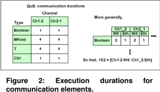
Figure 2: Execution durations for communication elements.
Inter processor communications have a duration that depends on the type of transmitted data (Figure 2, left-hand side). More generally, several channels (e.g., Ethernet and WiFi) may exist between two processors, associated with different costs (Figure 2, right-hand side). The communications may even be dissymmetric (e.g., ADSL where upstream and downstream communication costs are different).
3. Data flow representation
In UML 1.x activity graphs were just an informal specialization of state machines. Such a representation was not convenient for systems engineers. To address this issue, explicit representation of data and control
flows has been introduced through activity diagrams. Now, in UML 2.0, activities are first class concepts with their own diagrams. The semantics of activities is large enough to cover several domain-specific interpretations [2]. A more precise semantics can be given in profiles using the semantics variation points. In our case, the semantics is implied by systematic structural transformations that lead to a mathematically well-founded model: the Time Petri nets.
An activity is a UML behavior. It specifies a partial ordering of executions of subordinate behaviors, using control and data flow models. Activity diagrams support hierarchical description; subordinate behaviors are individual elements (actions) that can be invocation actions or structured activity nodes. The UML::Activities package consists of many packages. In order to provide automated transformations and to perform formal property verifications, we do not support all the activity model elements and constructs, but we require a precise semantics for the selected model elements. We use a synchronous semantics [11], well adapted to the kind of applications we focus on. This restriction can be imposed by stereotyping. We define «SActivity», a stereotype of Activity that conforms to the synchronous reactive model of computation. This choice requires this approach to be restricted to applications with deterministic executions or at least to applications for which a valid deterministic behavior can be derived. A synchronous system evolves in a sequence of non overlapping reactions in a lock-step manner. A typical synchronous execution scheme consists of a read phase (input acquisitions), a computation phase, and finally, a write phase (actuation). The sequence of these three phases is called a reaction and must be performed in isolation (i.e., the computation is blind to environment changes). Moreover a synchronous execution demands finite executions; it is loop free—the related SActivity is a Directed Acyclic Graph or DAG—and deterministic. Details about synchronous execution semantics are beyond the scope of this paper (see [12]).
Figure 3: Activity Diagram (top-level).
Figure 3 represents the application activity at the top level. In all figures we use the standard UML 2.0 notation [1]. For pins, only a small rectangle is normative. We choose, as most UML tools, to place an arrow inside the rectangle to indicate whether it is an input or an output pin. Modes are selected by a
DecisionNode. A DecisionInput is a behavior attached to a decision node, which selects one of its outgoing edges. The decision node is refined into an invocation action (decision), defined by its own activity diagram (not shown in this paper). Here, an action is a UML CallBehaviorAction that directly invokes a behavior. In our approach, a behavior is either elementary (e.g., isEqual, and thus specified by an elementary operation given in a table, see Figure 1) or further refined as an activity diagram (e.g. the M1 activity in Figure 3).
Access to information demands special actions, which can be resource and time consuming. We explicitly represent these accesses using two stereotypes of CallBehaviorAction: CallReadData for inputs, represented on Figure 3 by the box icon with an outgoing arrow, and CallWriteData for outputs. The 'which' stereotype attribute refers to the entity that conveys the value. This is a constant reference, not implying any object flow, and assigned to a ValuePin. Figure 3 is interpreted as follows: a value (the object m) is read from the sensor M and is used to decide whether to run in mode M1 or M2. Actions M1 and M2 are call behavior actions, specified in separate activity diagrams. For instance, activity M1 is described in Figure 4.
Figure 4: Activity Diagram (Mode M1).
4. From Data flow to Petri Net
Our main goal is to formally verify some non functional properties of the application. In this paper, we focus on time properties. For this purpose, we need to fulfill three requirements. First, give a formal semantics to each activity model element. Second, compose these semantics to derive the semantics of the SActivity. Third, take into account architectural constraints and non functional properties to be verified.
4.1. Hierarchical and Modular Time Petri Nets
To address the first requirement, Time Petri nets [13] have been preferred to the UML State Machines and Activities. Petri nets have well-established mathematical foundations (semantics) and offer rich analysis capabilities. Contrary to UML state machines, Petri nets support true concurrency. As for UML2.0 activity diagrams, though they are inspired from Petri nets, they lack a formal semantics.
We introduce Modular and Hierarchical Time Petri
Nets (MHTPN) to meet the second requirement, making
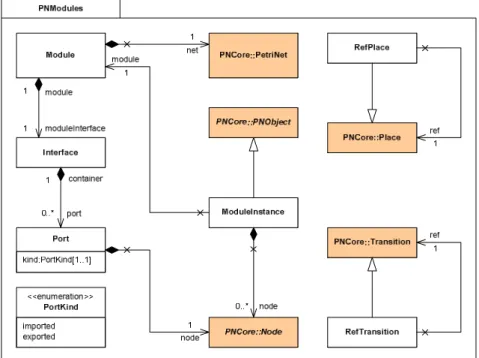
community is working on a model generic enough to cover all Petri Net formats (namely, the Petri Net Markup Language, PNML [14]). Our model, MHTPN, is specific to Time Petri nets, while PNML was designed to be completely generic. Thus, MHTPN is simpler and fits better our approach. It is organized in three packages. This hierarchical model (Figure 5) is built upon the classical flat model of Petri nets (Figure 6). In this latter
model, timing information (a special kind of cost specification) is attached to transition (Time Petri Net). A third package, not presented here, defines graphical features.
MHTPN modules, like PNML ones, compose through their interface, supporting both place and transition fusions.
Figure 5: Modular Time Petri Net Model.
Deriving MHTPNs from activity diagrams is driven by the structural transformations specified in Section 4.2. To satisfy the last requirement, we must take into account architectural constraints—distribution con-straints that result in communications—and temporal constraints. Section 4.4 explains how the MHTPNs are augmented by dedicated transformation patterns to make
communications explicit. Section 4.5 shows how temporal constraints are represented in the MHTPN.
4.2. Structural Transformations
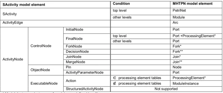
The structural transformations from SActivity model elements to MHTPN model elements are summarized in Table 1.
SActivity model element Condition MHTPN model element
top level PetriNet SActivity
other levels Module
ActivityEdge Arc
InitialNode Port
top level Port +ProcessingElement* FinalNode other levels Port
ForkNode Fork* DecisionNode Fork** JoinNode Join* ControlNode MergeNode Join** Pin Node ObjectNode ActivityParameterNode Port
∈
processing element tables ProcessingElement* Action∉
processing element tables ModuleInstance ActivityNodeExecutableNode
StructuredActivityNode Not supported * ModuleInstance : instances of modules predefined in a library.
** see the remark below.
Table 1: Behavior Transformation from SActivity model elements to MHTPN model elements.
Note that most of the SActivity model elements are transformed into module instances. We have defined a library of MHTPN modules suitable for expressing the temporal behavior. Figure 7 shows two examples: ProcessingElement and Join modules. The ProcessingElement module captures the temporal behavior of actions that represent elementary processing elements. In a module the grey-background part is the interface made of ports. The other part expresses the module behavior as a modular Petri net (i.e., it may use module instances as well). The central transition is fired when the processing element is executing, it takes inputs from the left hand-side place and produces outputs in the right hand-side place. This transition can only be fired when a resource is available; this resource is modeled by the place above the transition in the figure. This place, which is a ReferencePlace, may share—with another ProcessingElement—an actual place defined outside the module. With this first abstraction, the resource is released immediately. In section 4.4, we take duration into account through TimeIntervals associated with transitions. The Join MHTPN module is a very classical building block in Petri Nets. Nevertheless, it is important to note that the usage of such a module as a placeholder for an SActivity MergeNode is justified because we want to verify temporal properties. When several branches,
which take time, execute in parallel, the overall time spent is the maximal time of all branches. Using a Join results in computing the maximum, while using a Merge would have resulted in choosing the branch with the shortest time. Had we chosen to model another non functional property, like power consumption, we would have been bound to define another module—a Merge or any other adapted module—to represent an SActivity MergeNode.
Figure 7: Examples of modules from the MHTPN library.
Activity diagram focuses on the execution with a strong flow flavor and applies well to engineering systems. An activity expresses what to do but little where to do it. The activity diagram (section 3) specifies the algorithmic part of the application (section 2.1). Non functional constraints and the architectural aspects are
still to be captured. Distribution aspects and induced communications are also to be modeled. To this end, we introduce below two concepts—potential allocation and
communication processing elements—and the associated
transformations.
4.3. Potential Allocation
The processing and communication costs are related to a pair “elementary processing element, host”, which characterizes a potential allocation. A host is either a processor or a channel. An elementary processing element, associated with an elementary operation, is potentially deployed onto several targets (a set of hosts). For instance, oper3 can be deployed on processors P1 or P2. The respective costs are given in tables from Figure 1. A non elementary processing element, whose behavior is described by an Activity, is associated with a set of allocations resulting from the allocations of the subordinate actions. The cost associated with an Activity results from a semantic transformation that propagates allocation information. This process is explained below.
4.4. Communication processing element
Given the potential allocations for all elementary operations, we derive all potential communications. Some SActivity model elements require adding explicit communications; this is the case for actions that represent elementary processing elements and for the final node of the top-level SActivity. Communications must explicitly appear when they may have a cost. To avoid duplication, communications are systematically inserted before each input port of every elementary processing element. The communication cost varies depending on the potential allocations of both the target
and the source elementary processing elements. Since we are using a modular and hierarchical representation the source elementary processing elements may not be known when compiling the module. The source and its potential allocation will be discovered at elaboration
time after connecting module instances.
No communication is inserted for a user-defined Activity; its communication costs are eventually paid when used by an elementary processing element defined in the corresponding module.
A FinalNode is always translated into an output port. The FinalNode of the top-level SActivity needs a special transformation; it can be interpreted as a form of distributed termination, and as such, it may imply a communication cost. Therefore, a potential communication is inserted before it.
Alike elementary processing elements, communications take inputs, produce outputs, require a resource (i.e., communication media) and may take time. Therefore, both elementary processing elements and communications are represented with Processing-Element module instances.
4.5. Temporal constraints, architectural constraints and non-functional properties
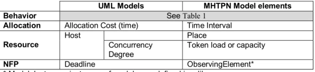
Table 2 summarizes how time constraints, architectural constraints and non-functional properties are modeled with the MHTPN modules. Execution durations from Figure 1 are integrated by associating a TimeInterval with the central transition of the corresponding ProcessingElement module instance (see Figure 7).
UML Models MHTPN Model elements
Behavior See Table 1
Allocation Allocation Cost (time) Time Interval
Place
Resource
Host
Concurrency Degree
Token load or capacity
NFP Deadline ObservingElement*
* ModuleInstance : instances of modules predefined in a library.
Table 2: Transformation rules.
The resource is held during a given amount of time, thus preventing other processing elements from using it at the same time. The output tokens are released at the end of the execution. Similarly, execution durations of communications (Figure 2) are integrated by associating a TimeInterval with the central transition of the corresponding communication ProcessingElement module instance. This characterization by a time interval is only sensible for dedicated real-time networks. More general communications would require stochastic models, not supported by TINA and MHTPN.
When a resource offers a concurrency degree higher than one, several tokens are put into the place that represents the resource, thus making the concurrent use of this resource possible.
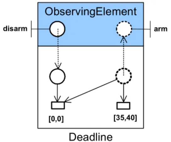
Finally the global deadline constraint is modeled using an ObservingElement module instance (Figure 8). This module is specifically designed for time properties. Had we chosen to verify another kind of non-functional property—like consumption for instance—we would have had to design another module.
ObservingElement
Deadline
[0,0] [35,40]
disarm arm
Figure 8: ObservingElement MHTPN module.
5. Time property analysis
For the purpose of time property analysis we use the time Petri net analyzer (Tina) [15], which supports both timed and untimed nets. However, Tina does not support hierarchical descriptions. We have built a tool that allows for graphical composition of MHTPN modules. It exports flattened modules into a Tina-compatible format. Section 5.1 shows how Tina is used to check time properties. Section 5.2 briefly describes the software environment we have built as a prototype to demonstrate the feasibility of our approach.
5.1. Property checking
In order to be analyzed, the MHTPN generated by model transformations is flattened into a Time Petri Net, which is a prerequisite for Tina. From a Time Petri Net, Tina generates various behavioral graphs, on which analyses can be conducted. The simplest exploration reports unbounded places and dead transitions. Behavioral graphs can be efficiently shared and exchanged as a Kripke Transition system for advanced analyses
Tina offers a large choice of analysis methods dealing with various levels of abstraction. The exploration can be exhaustive, which is often the case for our acyclic Petri nets, or partial. The violation of safety properties can be detected on the fly (i.e., while generating the behavioral graph). Notice that deadline is a form of safety property, also known as ‘bounded liveness’. When a property is violated, a counter example is generated. Tina also allows the designer to express the expected properties in temporal logic formulas (Linear Time Logic—LTL—or Computational Tree Logic star— CTL*—), which are then verified by model-checking techniques.
Our MHTPN library modules are devised so as dead transitions reveal property violations or structural inconsistency. For example, we can identify impossible allocations, or check whether or not the deadline
constraints are met. For the application of Section 2, using LTL formulas, the analysis is able to assert the following properties:
1. There is no valid allocation with a deadline constraint less than 38 time units.
2. To meet the strong deadline of 38 time units, oper2, oper3 and outpY must be executed on P2, while inpC can be executed either on P1 or P2.
3. To meet the weaker deadline constraint of 40 time units, oper2 must be executed on P2 but there is no constraint for other potential allocations.
5.2. Software environment
We have started to implement a tool suite that supports the four steps of the transformation chain. The first step concerns the capture of the activity diagram, of architectural constraints and of non-functional properties. The second step is the transformation of SActivity diagrams into MHTPN. In the third step, the MHTPN is flattened and exported to Tina as explained in the previous section. Tina is used to perform the fourth step and the result provided is brought back inside our tool for interpretation.
Concerning the actual implementation, the first two steps imply building a UML modeling tool and using a mature model transformation technology; they are still under development and the related actions were performed manually on the example presented. The third step has been implemented first because it involves the manipulation of hundreds of nodes even for small examples, while previous steps apply to more abstract models, making them simpler to handle.
We have built an Eclipse plug-in that captures the MHTPN, flattens it and exports it in a format accepted by Tina. The MHTPN metamodels shown in Figure 5 and Figure 6 have been captured using an EMF Ecore model. The EMF technology generates the business model code, XML generators and parser; it thus provides a support for making the models persistent. The XML files produced follow an XML schema also generated by EMF. Even though EMF also provides tree-based editors that follow the model description, we have found them not sufficiently user friendly for our application. Then, we have implemented upon the EMF-generated business model code, a graphical interface using the GEF methodology. More details about the Eclipse framework and the related EMF and GEF projects are available on the Eclipse web site [16].
6. Conclusion
This paper has shown a way to use UML and model transformations to derive an analysis model from a UML functional description. First, the functionality of the application is expressed as a stereotyped UML activity diagram tailored for synchronous reactive execution. Following the model-driven approach, this model passes
through a series of transformations resulting in a model amenable to formal analyses.
For property analysis, the semantics of UML 2.0 is not sufficiently precise (many semantic variation points, no formal definition). This is a deliberate choice made by the standard to be widely applicable. When a precise domain or fine property analyses are targeted, the semantics has to be strengthened within a profile. This is what we have done to model distributed control applications with several potential allocations of operations to hardware/software execution supports. The semantics of UML 2 activity diagrams has been revisited to remove variations points and introduce “synchronous” evolutions. Details about this profile are available in a technical report [17]. For analysis, since this paper focuses on the temporal correctness of applications with concurrent evolutions, we have chosen Petri Nets as the analysis domain and especially, modular and hierarchical time Petri nets.
Diagram interchanges and model transformations have been implemented in Java, within the Eclipse framework. Meta-models have been captured using an EMF Ecore model. Temporal properties are analyzed by Tina, a time Petri net analyzer. Reachability analysis tools of Tina establish the existence of a valid allocation meeting temporal constraints. More complex properties can be expressed as temporal logic formulas (LTL formulas) and formally analyzed by model-checking techniques. The Tina tool box provides the behavioral graph generator, facilities to specify temporal logic formulas, and connections to several model-checkers. For the example studied in the paper, with the given parameters, we have established that a given operation must necessarily be allocated to a given processor in order to meet the deadline. This leads to a reduction of the possible allocations to be explored. Once the adequate solutions are better characterized, we may export pertinent information, extracted from UML models, to other analysis tools. For instance, we could easily export the algorithm and architecture models to SynDEx [9] for further optimization and generation of the real-time distributed code.
This paper has illustrated how to associate time Petri nets with our library elements. We have used Petri net models as behavioral models. However, they cannot easily capture preemptive behaviors. We plan to use more expressive formalisms. In the future, to make the best of the underlying synchronous hypotheses, we intend to use the industrial synchronous language Esterel /Scade [18] and its validation tools, or the Polychrony platform [19].
References
[1] “Unified Modeling Language: Superstructure. V 2.0”. OMG document formal/05-07-04. April 2005. http://www.omg.org/docs/formal/05-07-04.pdf [2] B. Selic. “On the Semantic Foundations of
Standard UML 2.0”, SFM-RT 2004, LNCS 3185, Springer-Verlag, pp. 181-199, 2004.
[3] Tony Clark, Andy Evans, Stuart Kent, Steve Brodsky, Steve Cook, A feasibility Study in Rearchitecturing UML as a Family of Languages using a Precise OO Meta-Modelling Approach, version 1.0, available from www.puml.org, September 2000.
[4] H. Störrle. Semantics and Verification of Data Flow in UML 2.0 Activities. Electronic notes in Theoretical Computer Science, 127(4), pp. 35-52, 2005.
[5] L. Apvrille, J.-P. Courtiat, C. Lohr, P de Saqui-Sannes, A Real-Time UML Profile Supported by a Formal Validation Toolkit, IEEE Transactions on Software Engineering, Vol 30, N° 7, pp 473-487, July 2004
[6] “UML Profile for Schedulability, Performance, and Time, version 1.1”. OMG document formal/2005-01-02, January 2005, http://www.omg.org/docs/-formal/05-01-02.pdf
[7] “UML Profile for Modeling and Analysis of Real-Time and Embedded systems (MARTE) RFP”, OMG Document realtime/05-02-06, February 2005, http://www.omg.org/docs/realtime/05-02-06.pdf
[8] L. Cai and D. Gajski, “Transaction Level Modeling: An Overview”, Proceedings of the International Conference on Hardware/Software Codesign & System Synthesis, Newport Beach, CA, October 2003.
[9] T. Grandpierre, Y. Sorel. “From Algorithm and Architecture Specifications to Automatic Generation of Distributed Real-Time Executives: a Seamless Flow of Graphs Transformations”. MEMO¬CODE2003, Formal Methods and Models for Codesign Conference, Mont Saint-Michel, France, June 2003.
[10] “UML profile for Systems Engineering RFP”, OMG Document ad/03-03-41, September 2003, http://www.omg.org/docs/ad/03-03-41.pdf
[11] A. Benveniste, P.Caspi, S. Edwards, N. Halbwachs, P. Le Guernic, R. De Simone “The synchronous languages 12 Years Later”, Proc. of the IEEE, Vol.91, n° 1, pp. 64—83, 2003.
[12] R. De Simone, C. André. “Towards a Synchronous Reactive UML subprofile?”, International Journal on Software Tools for Technology Transfer (STTT), Springer-Verlag, ISBN=1433-2779 (Paper) 1433-2787 (Online). DOI:10.1007/s10009-005-0206-9, December 2005.
[13] The Petri Nets World. http://www.informatik.uni-hamburg.de/TGI/PetriNets
[14] J. Billington, S. Christensen, K. van Hee, E. Kindler, O. Kummer, L. Petrucci, R. Post, C. Stehno, and M. Weber. “The Petri Net Markup Language: Concepts, Technology, and Tools”, ICATPN 2003, Eindhoven, June 2003. http://www.informatik.huberlin.de/top/pnml/downl oad/about/PNML_CTT.pdf
[15] B. Berthomieu, P-O. Ribet, F. Vernadat, “The tool TINA – Construction of abstract state space for Petri net and Time Petri Nets", Int. Journal of
Production Research, Vol. 42, n° 14, pp. 2741— 2756. July 2004. http://www.laas.fr/tina
[16] The Eclipse project, http://www.eclipse.org [17] C. André, F. Mallet, M-A. Peraldi-Frati.
“Non-functional Property Analysis using UML2.0 and Model Transformations”, Research Report n° 5913, INRIA (F), May 2006.
[18] Esterel Studio./Scade http://www.esterel-techno-logies.com
[19] P. Le Guernic, J-P. Talpin, J-C. Le Lann. “Polychrony for system design”, Journal of Circuits, Systems and Computers, 12(3), pp 261-304, April 2003.
![Figure 3 represents the application activity at the top level. In all figures we use the standard UML 2.0 notation [1]](https://thumb-eu.123doks.com/thumbv2/123doknet/13511119.416080/4.892.92.428.834.969/figure-represents-application-activity-level-figures-standard-notation.webp)