Entropies and the Anthropocene crisis

(1)

HAL Id: hal-02398756

https://hal.archives-ouvertes.fr/hal-02398756v4

Submitted on 17 May 2021

HAL is a multi-disciplinary open access archive for the deposit and dissemination of sci-entific research documents, whether they are pub-lished or not. The documents may come from teaching and research institutions in France or abroad, or from public or private research centers.

L’archive ouverte pluridisciplinaire HAL, est destinée au dépôt et à la diffusion de documents scientifiques de niveau recherche, publiés ou non, émanant des établissements d’enseignement et de recherche français ou étrangers, des laboratoires publics ou privés.

Entropies and the Anthropocene crisis

Maël Montévil

To cite this version:

Maël Montévil. Entropies and the Anthropocene crisis. AI & Society: Knowledge, Culture and Communication, Springer Verlag, 2021. �hal-02398756v4�

(2)

Entropies and the Anthropocene crisis

Maël Montévil*

Abstract

The Anthropocene crisis is frequently described as the rarefaction of resources or resources per capita. However, both energy and minerals correspond to fundamentally conserved quantities from the perspective of physics. A specific concept is required to understand the rarefaction of available resources. This concept, entropy, pertains to energy and matter configurations and not just to their sheer amount.

However, the physics concept of entropy is insufficient to understand biological and social organizations. Biological phenomena display both historicity and systemic properties. A biological organization, the ability of a specific living being to last over time, results from history, expresses itself by systemic properties, and may require generating novelties The concept of anti-entropy stems from the combination of these features. We propose that Anthropocene changes disrupt biological organizations by randomizing them, that is, decreasing anti-entropy. Moreover, second-order disruptions correspond to the decline of the ability to produce functional novelties, that is, to produce anti-entropy.

Keywords: entropy, anti-entropy, resources, organization, disruption, Anthropocene

Cite as: Montévil, Maël. 2021. “Entropies and the Anthropocene Crisis.” AI and Society. doi: 10.1007/s00146-021-01221-0 Preprint:https://montevil.org/publications/ articles/2021-Montevil-Entropies-Anthropocene/

1 Introduction

Despite cases of denial, citizens and governments increasingly acknowledge the Anthropocene as a crisis. Nevertheless, this crisis requires further theoretical characterization. For example, geological definitions of the Anthropocene mostly build on human productions that could be found in future geological strata with indicators such as chicken bones, radionuclides, and carbons. However, these operational definitions for stratigraphy do not contribute much to understanding the underlying process and how to produce the necessary bifurcations. Beyond stratigraphy, in the second “warning to humanity” signed by more than 15000 scientists, the arguments are strong but build mostly on a single line of reasoning. The authors exhibit quantities that are growing or shrinking exponentially (Ripple et al , 2017), and it stands to reason that such a trend cannot persist in a finite planet. This line of reasoning is commonplace in physics and shows that a change of dynamics is the only possibility. For example, the said quantities may reach a maximum, or the whole system may collapse. However, are these lines of reasoning sufficient to understand the Anthropocene crisis and respond adequately to it?

Several authors have specified the diagnosis of the Anthropocene. They argue that this crisis is not a result of the Anthropos sui generis, but the result of specific social organizations. Let us mention the concept of capitalocene for which the dynamics of capital is the decisive organizational factor (Moore, 2016). The capital opened the possibility of indefinite accumulation abstracted from other material objects. Along a similar line, the concept of plantationocene posits that the plantation is the damaging paradigm of social organizations and relationships to other living beings (Haraway, 2015; Davis et al , 2019). In both cases, the focus is on human activities and why they are destructive for their conditions of possibility. These accounts provide relevant insights, but we think they are insufficient in their articulation with natural sciences.

To integrate economics and natural processes, Georgescu-Roegen (1993) emphasized the theoretical role of entropy in physics. Economists should part with the epistemology of classical mechanics where conservation principles and determinism dominate. In thermodynamics, the degradation of energy is a crucial concept: the irreversible increase of entropy. Methodologi-cally, the implication is that economists should take into account the relevant knowledge about natural phenomena instead of working on self-contained mathematical models representing self-contained market processes.

This work has been reinterpreted by Stiegler (2018, 2019). B. Stiegler argues that the Anthro-pocene’s hallmark is the growth of entropies and entropy rates at all levels of analysis, including the biological and social levels. In this paper, we will discuss several aspects of this idea, focusing on mathematized situations or situations where mathematization is within sight. Entropy leads

(4)

to a shift from considering objects that are produced or destroyed — even energy is commonly said to be consumed — to considering configurations, organizations, and their disruptions.

We first explain why entropy is a critical concept to understand the “consumption” of energy resources. We provide a conceptual introduction to the thermodynamic concept of entropy that frames these processes in physics. We will also discuss resources like metals and argue that the property impacted by biological and human activity is not their amount on Earth but their configuration. Concentrations of metals increase when geological processes generate ore deposits. On the opposite, the use of artifacts can disperse their constituents. Last, compounds dispersed in the environment can be concentrated again by biological activities, leading to marine life contamination with heavy metals, for example.

To address biological organizations and their disruptions, we first develop several theoretical concepts. The epistemological framework of theoretical biology differs radically from equilibrium thermodynamics — and physics in general. We introduce the concepts of anti-entropy and anti-entropy production that mark a specific departure from thermodynamic equilibrium. We show that they enable us to understand critical destructive processes for biological and human organizations.

2 Entropy in physics and application to available resources

In this section, we will discuss two kinds of resources relevant to the economy and show that the proper understanding of these resources requires the concept of entropy in the physical sense of the word. The first case that we will discuss is energy, and the second is elements such as metals. 2.1 Energy and entropy

The stock of energy resources is commonly discussed in economics and the public debate. However, it is a fundamental principle of physics that energy is conserved. It is a physical impossibility to consume energy stricto sensu. For example, the fall of a ball transfers potential energy into kinetic energy, and if it bounces without friction, it will reach the initial height again, transforming kinetic energy back into potential energy. This remark is made repeatedly by physicists and philosophers but does not genuinely influence public discourses (Mosseri and Catherine, 2013). Georgescu-Roegen (1993) and authors who built on his work are an exception.

To dramatize the importance of this theoretical difficulty, let us mention that the increase in a body’s temperature implies increased internal energy. Heat engines, including thermic power plants, are a practical example of this: they transform heat into useful work (e.g., motion). We are then compelled to ask an unexpected question. Why would climate change and the subsequent increases in temperature not solve the energy crisis?

2.1.1 Thermodynamic entropy

The greenhouse effect keeps the energy coming from the Sun on Earth, and at the same time, the shrink of resources such as oil leads to a possible energy crisis. The main answer to this paradox is that not all forms of energy are equivalent.

Let us picture ourselves in an environment at a uniform temperature. In this situation, there is abundant thermic energy environing us, but there are no means to generate macroscopic motions from this energy. We need bodies at different temperatures to produce macroscopic motions. For example, warming up a gas leads to its expansion and can push a piston. If the gas is already warm, it cannot exert a net force on the said piston. It is the warming up of the gas that generates usable work, and this process requires objects with different temperatures.

An engine requires a warm and a cold source, a temperature difference. This rationale led to design cycles where, for example, a substance is warmed up and cooled down iteratively. These

(5)

cycles are the basis of heat engines. XIXth century physicists, in particular, Carnot and Clausius, theorized these cycles. When generating macroscopic motion out of thermic energy, the engine’s maximum efficiency is limited, and physicists introduced entropy to theorize this limitation.1 The efficiency depends on the ratio of temperatures of the cold and the warm sources. When the temperatures tend to become equal, the efficiency decreases and tends to zero. As a side note, nuclear power plants use the same principle, where the warm source result from atomic fission, and the cold source is a river or the sea. It follows that the higher the temperature of their surroundings is, the less efficient they are. Incidentaly, it also follows that nuclear powerplant are often close to the sea, which can lead to some problems in a context were the sea level is expected to rise.

Now, let us consider warm water and cold water and pouring them together in a pot. After some time, the water will reach a uniform temperature, and we have lost the chance to extract mechanical work out of the initial temperature difference. This phenomenon is remarkable because it displays a temporal direction: we have lost the ability to do something. Theoretically, this kind of phenomenon defines a time arrow that classical mechanics lacks.2 Likewise, it is possible to generate heat out of mechanical work by friction, including in the case of electric heaters, but, as we have seen, the opposite requires two heat sources at different temperatures.

Following the first principle of thermodynamics, energy is a conservative quantity. Being conservative is a different notion from being conserved. A conserved quantity does not change over time in a system. For example, the number of water molecules in a sealed bottle is conserved. This property pertains both to the quantity discussed and the nature of the system’s boundaries. By contrast, being conservative pertains mainly to the quantity itself. A conservative quantity can change in the intended system, but only via flows with the outside, and the change corresponds precisely to the flow. A system’s energy is not necessarily conserved; it can decrease if it is released outside or increase if some energy comes from outside. The same is not exactly valid for the number of water molecules because they can disappear in chemical reactions. Instead, chemists consider that the number of atoms, here hydrogen and oxygen, is conservative.

In this context, what is entropy? The classical thermodynamic perspective defines entropy as a quantity describing the state of a system together with other quantities like energy, volume, …Physicists used to think of heat as the exchange of an abstract fluid, the “caloric”; however, the possibility of a complete transformation of work into heat and the partial conversion of heat into work is not amenable to such a definition. Nevertheless, the notion of fluid remains partially relevant to understand what entropy abstractly is. Entropy is proportional to the size of a system, like mass or energy. Entropy can be exchanged, and in special conditions called reversible, entropy is conservative, like energy.

However, the difference between entropy and energy is that entropy tends to increase towards a maximum in an isolated system, following the second principle of thermodynamics. This statement has two implications: i) entropy is not conservative in general, and ii) the non-conservative changes of entropy are only increases. In reversible situations, entropy is conservative. By contrast, irreversibility leads to the concept of entropy production: a net increase of entropy that does not stem from flows with the surroundings.

Here again, being conservative is not the same as being conserved, and entropy production is the departure from entropy being conservative. Nicolis and Prigogine (1977) showed that a system such as a flame can produce entropy continuously and still be stationary if the resulting entropy flows to the surroundings. Here, the entropy of the system is conserved, but it is not conservative. Similarly, the entropy of a system can decrease when work is used to this end. For example, centrifugation separates compounds of a gas or a liquid.

1_{This efficiency is defined as the work produced divided by the heat taken from the warm source.}

2_{The concept of a time arrow is somewhat abstract. Intuitively, there is a time arrow if we can tell whether a movie}

(6)

The second principle of thermodynamic also captures the idea that heat can only go from warm bodies to cold bodies. The entropy change due to a heat exchange𝑄 is 𝑑𝑆 = 𝑄/𝑇, where 𝑆 is the entropy, and 𝑇 is the temperature. Then, if we have a isolated system with two bodies at temperature𝑇_ℎ> 𝑇_𝑐, exchanging heat, then𝑑𝑆 = 𝑄_𝑐→ℎ/𝑇_ℎ+ 𝑄_ℎ→𝑐/𝑇_𝑐. We assume that the objects only exchange heat between each other so that𝑄_𝑐→ℎ= −𝑄_ℎ→𝑐. The only way for𝑑𝑆 to be positive is if𝑄_ℎ→𝑐is positive; that is, the energy is going from the warm body to the cold body. In classical thermodynamics, the central concept is thermodynamic equilibrium. At equilib-rium, there are no macroscopic net fluxes within the system and with the system surroundings. For example, if we consider an open room, thermodynamic equilibrium is met when temperature, pressure, and other variables are homogeneous and the same as the surroundings. There are always exchanges of gas with the surroundings, but on average, there are no fluxes. By contrast, Nicolis and Prigogine (1977) describe stationary configuration far from thermodynamic equilibrium where there is a net flow of entropy from the system to the surroundings.

Thermodynamic equilibrium is typically the optimum of a function called a state function. These functions are the combination of state variables appropriate for a given coupling with the system’s surroundings. For example, entropy is maximal for an isolated system at thermodynamic equilibrium. Another example, Helmholtz free energy𝐹, describes the usable work that can be obtained from a system at constant temperature and volume. Let us discuss its form,𝐹 = 𝑈 − 𝑇𝑆, where𝑈 is the internal energy, 𝑇 the temperature, and 𝑆 the entropy. 𝑇𝑆 corresponds typically to the energy in the thermic form so that𝐹 is the energy minus the internal energy in thermic form. Spontaneously, Helmholtz’s free energy will tend to a minimum. This property is used in engineering to design processes leading to the desired outcome.

Helmholtz free energy is not the most commonly used function. Consider a battery in ordinary conditions; its purpose is to provide electrical work to a circuit, a smartphone, say. Part of the battery’s work is its dilation, which will push air around it. However, this is not genuinely useful. This kind of situation leads to the definition of Gibbs energy, the maximum amount of non-expansion work that can be obtained when temperature and pressure are set by the surroundings,𝐺 = 𝐹 + 𝑝𝑉, where 𝑝 is pressure and 𝑉 is volume.

In these examples, couplings with surroundings are a manifestation of technological purposes. Sometimes, the concept of exergy is used to describe available energy in general. Unlike Helmholtz and Gibbs free energy, exergy is not a state function because it depends on the quantities describing the system’s surroundings, such as external temperature. In other words, calculus on state function like free energies only depends on initial and final conditions. By contrast, work, heat, or exergy balance depend on the transformation path, not just initial and final states. It follows that exergy depends on circumstances and cannot be aggregated in general. Practically, this means that the available energy of a nuclear power plant with a given amount of nuclear fuel is not just a property of this power plant or fuel; it depends on external temperature (precisely, water input temperature).

Classical mechanics is deterministic and provides the complete trajectories of the objects described. By contrast, thermodynamics only determines the final state of a system by minimiz-ing the appropriate function. Since this state is sminimiz-ingularized mathematically as an extremum, theoreticians can predict it. The epistemological efficacy of this theory lies precisely in the ability to determine final states. A system can go from the initial situation to the final situation by many paths, but the outcome is the same. Calculations are performed on well-defined, theoretical paths, whereas the actual paths may involve phenomena such as explosions where variables like entropy are not well-defined (they are defined again at equilibrium).

Classical thermodynamics is about final states at thermodynamic equilibrium. There is no general theory for far from thermodynamic equilibrium conditions. The study of these situations may or may not use thermodynamic concepts. For example, biological evolution or linguistic phenomena all happen far from thermodynamic equilibrium, but their concepts are

(7)

not thermodynamic. By contrast, non-equilibrium thermodynamics, such as the work of Nicolis and Prigogine (1977), is a direct extension of equilibrium thermodynamics. Unlike classical thermodynamics, these approaches need to introduce an accurate description of the dynamics. A standard method assumes that small parts of the system are at or close to thermodynamic equilibrium but that globally the system is far from it.

To sum this discussion up, entropy is abstractly similar to fluids to an extent. This analogy’s shortcoming is that entropy is not conservative and spontaneously tends to a maximum in an isolated system. We do not genuinely consume energy; we are producing entropy. However, this does not lead to a straightforward accounting of entropy production on Earth. Earth is far from equilibrium, and its entropy is not well defined. Locally, exergy (usable energy) is not a state function, and we cannot aggregate exergy between systems with a different nature. Nevertheless, in comparing physically similar, local processes, entropy production, and exergy are relevant and necessary concepts.

In this context, it is interesting to note that an increase in temperature leads to an increase in entropy. As such, if Earth’s entropy were defined, global warming would increase it. At the same time, Earth is exposed to the cold of space vacuum and loses heat this way. The greenhouse effect slows down this process and slows down the corresponding entropy production (released in open space). Accordingly, if we had a machine using the heat of the Earth’s surface as a warm source and the open space as a cold source, global warming would lead to more usable energy. Of course, this principled analysis has no practical counterpart. With this last example, we aim to emphasize again that the assessment of entropy and entropy production should be performed in the context of technological or biological processes.

2.1.2 Microscopic interpretations of entropy

The thermodynamic perspective described above is somewhat abstract; however, it has two microscopic interpretations introduced by Boltzmann and Gibbs. Debates on which of this interpretation is more fundamental are still ongoing, and their prevalence also has geographical differences (Goldstein et al , 2020; Buonsante et al , 2016). Despite their conceptual differences, for large isolated systems, they lead to identical mathematical conclusions. Moreover, both are bridges between microscopic and macroscopic descriptions. Here, we assume that the microscopic description is classical, deterministic dynamics, and we do not discuss the quantum case.

Let us start with Boltzmann’s interpretation of entropy. We consider gas in an insulated container so that its energy is constant. At the microscopic level, molecules move and bump on each other and the container’s walls chaotically. At this level, particles are described by their positions and velocities in three dimensions. These numerous quantities define together the microstate,𝑋, and the microspace, i.e., the mathematical space of possible microstates. Let us insist that the microstate is not small; it describes all particles, numbering typically1023, thus the whole system. Then, we can define the possible macrostates. For example, we posit that one macrostate corresponds to the molecules’ uniform distribution at a given scale and with a given precision. We can define another macrostate where all the particles are in the container’s corner and one that encompasses all other possibilities. Depending on the microstate𝑋, we will be in one of the three possible macrostates.

Let us follow Boltzmann and callΩ(𝑋) the microspace volume that corresponds to the same macrostate than𝑋. There are two crucial points in Boltzmann’s reasoning on Ω.

First, the microscopic volume of a particular macrostate is overwhelmingly higher than the one of others. This situation is a mathematical property that stems from the huge number of particles involved. As a mathematical illustration, let us throw coins. Heads are 1, and tails are 0. The macroscopic variable is the average of the result after a series of throws, which can go from 0 to 1. The first macrostate (𝑀₁) is met when this average is between 0.49 and 0.51. All other

(8)

ABC D E Macrostates

Ω(X)

X

Figure 1: Illustration of Boltzmann entropy. Here, the microspace is represented schematically in 2 dimensions, and colors represent the corresponding macrostates. The system starts from a microstate associated with macrostate𝐴. It explores microstates uniformly and soon arrives in positions corresponding to the macrostate𝐸 because most microstates correspond to 𝐸. For a microstate𝑋, the number of configurations leading to the macrostate is Ω(𝑋) (in light blue). Note that in physics, the microspace is not in 2 dimensions but has a huge number of dimensions — it is often the space of positions and momenta of all molecules, which leads to 3 + 3 = 6

quantity per particle.

possibilities lead to the other macrostate (𝑀₂). With four throws we get, for example0011 → 0.5 (𝑀₁),0110 → 0.5 (𝑀₁),0010 → 0.25 (𝑀₂),1110 → 0.75 (𝑀₂),1110 → 0.75 (𝑀₂) and so on. The macroscopic outcomes are quite random. However, for 10000 throws, with simulations, we get0.493 (𝑀₁),0.499 (𝑀₁),0.505 (𝑀₁),0.507 (𝑀₁),0.498 (𝑀₁) and so on. The system is always in the first macrostate, even though it covers a small part of the possible macroscopic values. This outcome stems from the combinatorics that leads an overwhelming number of possibilities to correspond to a specific macrostate, marginalizing alternatives.

Second, Boltzmann assumes molecular chaos: the system explores the microspace uniformly. It follows that the time spent by the system in a given macrostate is proportional to the microscopic volume of this macrostate.

Since one macroscopic possibility corresponds to an overwhelming part of the microspace, the system will spontaneously go into this domain and remain there except for possible, rare, and short-lived periods called fluctuations. The largest the number of particles, the rarest fluc-tuations are. In typical sifluc-tuations, the number of particles is not 4 or 10000, but is closer to 1000000000000000000000; therefore, fluctuations do not matter.

The number of microstatesΩ(𝑋) tends to a maximum with vanishingly rare fluctuations. This result interprets the second principle of thermodynamics, which states that entropy cannot decrease in an isolated system. For example, why do all air molecules not go to one corner of the room? Because all microscopic situations are equally likely and far more microscopic configurations correspond to a uniform air concentration than any other macrostate, see figure 1.

(9)

playing pool, the initial configuration is improbable, and we spontaneously think that somebody had to order the pool balls for them to be in a triangle shape. After striking them, their con-figuration becomes more uniform, and we acknowledge that it is the result of multiple random collisions. The same qualitative result will follow if we throw balls randomly on the table. It is the same for velocities. Initially, only the ball struck is moving, and all others are still. After the collision, the kinetic energy is distributed among the balls until friction stops them. Of course, the game’s goal is to go beyond randomness, and players aim for balls to reach specific locations. The number of possibilitiesΩ is a multiplicative quantity. For example, if we throw a coin, there are2 possibilities, but if we throw three coins, there are 2 × 2 × 2 = 8 possibilities. This mathematical situation does not fit with the idea that entropy is proportional to a system’s size, which is part of its classical definition. The logarithm function transforms multiplications into additions, so log(Ω1× Ω2) = log(Ω1) + log(Ω2). Then log(Ω) fits the properties of classical

entropy, and we can state with Boltzmann that:

𝑆 = 𝑘𝐵log(Ω(𝑋)), where 𝑘𝐵is a constant

Of course, there are many refinements of this entropy definition. Here, we considered that the total energy is conserved, whereas it is not always the case. Then, the definition of macrostates must include energy.

Gibbs proposed a different conceptual framework to interpret thermodynamic entropy (Gold-stein et al , 2020; Sethna, 2006). Instead of studying the state of a single system, Gibbs study an ensemble of possible systems describing microstates and their probabilities.

In particular, the fundamental postulate of statistical mechanics states that all microstates with the same energy have equal probability in an isolated system. This ensemble is called the microcanonical ensemble — this is Boltzmann’s hypothesis in a different conceptual context.

Then, except for temperature and entropy, the macroscopic quantities are averages of the microscopic quantities computed with the probabilities defining the ensemble. The Gibbs entropy is defined by:

𝑆 = −𝑘𝐵� 𝑖

𝜌𝑖log(𝜌𝑖), where 𝜌𝑖is the probability of the microstate𝑖

Despite their formal similarity, Gibbs and Boltzmann’s formulations have a critical difference. In Boltzmann’s formulation, a single microstate has an entropy: a microstate corresponds to a macrostate, this macrostate corresponds to many microstates, and how many define the entropy of the said microstate. By contrast, Gibbs framework is not about individual microstates; it considers all possible microstates simultaneously, and entropy is a property of their probability distribution. For example, when the system is isolated, and its total energy is constant, all microstates with the same energy have equal probability, which maximizes the entropy.

In a nutshell, the entropy being maximal is a property of the state of the system for Boltzmann. By contrast, it is a property of an ensemble of systems for Gibbs, and more specifically, it is a property of the associated probabilities. In mathematically favorable conditions (infinite number of particles), the outcome is the same despite this significant conceptual difference.

Microscopic interpretations of entropy present a hidden challenge. Liouville’s theorem states that the probabilities in an initial volume in the microspace are conserved over the dynamics. It follows that this volume cannot shrink or expand over time. Taken as is, this would mean that the entropy cannot increase over time — an embarrassing result when aiming to interpret the second principle of thermodynamics.

The leading solution to this problem is a procedure called coarse-graining. Let us introduce it by analogy. Does sprayed water occupy a larger volume than when it was in the tank of a spray bottle? Once water is sprayed, a hand moved in the air affected is going to be wet. From the

(10)

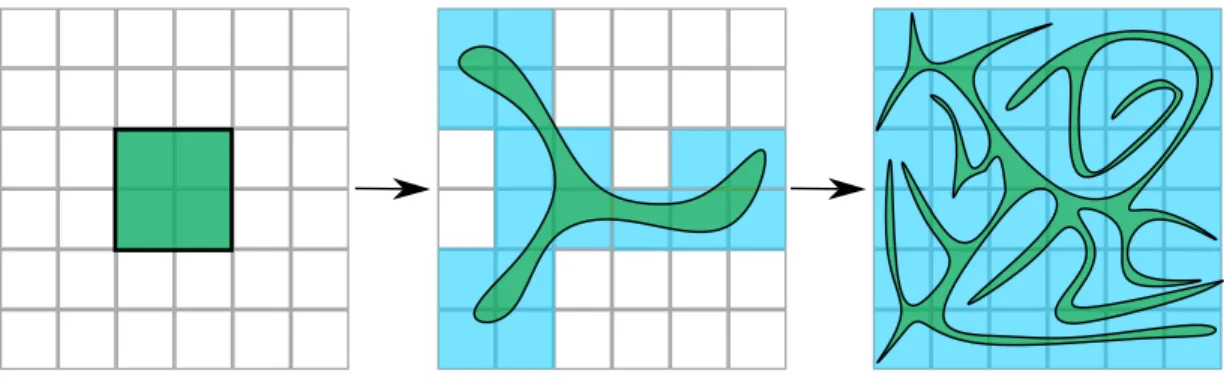
Figure 2: Coarse-graining versus Liouville’s theorem. As in figure 1, space is represented schemati-cally in 2 dimensions. The microspace is coarse-grained by a grid. The systems are initially in a small part of the microspace, which corresponds to four coarse-grained boxes. After some time, the initial volume has deformed without expanding at the fine-grained level in green. However, the coarse-grained volume occupied by the systems has expanded in blue. After more time, the fine-grained volume has become highly convoluted and meets the whole coarse-grained space, in blue. The growth of the coarse-grained volume occupied by the systems is the argument explaining the growth of entropy.

perspective of the hand, water occupies a vast volume of air. Nevertheless, the actual liquid water volume remains the same; water has just been dispersed, not added. This example illustrates two ways to understand the water volume: the fine-grained water volume that remains the same and the volume from the coarse-grained perspective of the hand — this volume has increased. Mathematically, if we partition space into boxes, all these boxes will contain some sprayed water. This procedure is called coarse-graining. The fine-grained water volume remains the same, but the coarse-grained volume has expanded (figure 2). In physics, coarse-graining follows this logic; however, space and volume no longer pertain to the three-dimensional physical space. Instead, these notions refer to the abstract microspace that typically corresponds to all particles’ position and momenta in the system.

Technically, the microstates are not represented individually in entropy calculation because entropy would not change over time due to Liouville’s theorem. Instead, physicists use a coarse-grained representation of the system. The dynamics still preserve the fine-coarse-grained volume; however, the latter deforms, gets more and more convoluted over time, and meets more and more coarse-grained volumes (the boxes). As a result, the coarse-grained volume increases, and so does the entropy (figure 2).

Let us make several supplementary remarks.

First, in classical thermodynamics, the second principle is imperative: an isolated system’s entropy cannot decrease. By contrast, in Boltzmann’s formulation, entropy can also decrease albeit overwhelmingly rarely. In Gibbs formulation, the equilibrium probabilities remain as such, so entropy can only increase.

Second, the concept of entropy in physics pertains to physics. The hallmark of this theoretical context is the use of the constant𝑘_𝐵.𝑘_𝐵is the bridge between temperature, heat, and mathematical entropy since an exchange of heat leads to 𝑄/𝑇 = 𝑑𝑆 = 𝑘_𝑏𝑑 log Ω. Specifically, 𝑘_𝐵 has the dimension of energy divided by temperature. Sometimes, a similar mathematical apparatus can be used, for example, to study flocks of birds or schools of fishes (Mora and Bialek, 2011); however, this use is an analogy and does not convey the same theoretical meaning (Montévil, 2019c). The absence of𝑘_𝐵is evidence of this fact. Along the same line, in physics, the space of possible microscopic configurations inherited from mechanics is position and momenta, and other aspects can be added, such as molecular vibrations or chemical states.

(11)

Third, the relationship between a system and its coupling is complex. We have emphasized that exergy, in general, depends on variables describing its outside; therefore, it depends on transformation paths and is not a state function. Even for state functions, macroscopic systems’ descriptions depend on their couplings precisely because the state function that leads to predictions depends on the couplings. Along the same line, with Gibbs’s interpretation, the system’s statistics entirely depend on the couplings; it is impossible to describe the macroscopic system without them. A change of couplings will require a change of statistics. Boltzmann’s interpretation is more complex in that regard. The definition of macroscopic variables and coarse-graining depend on the couplings; however, the microscopic definitions are somewhat independent; for example, they may rely on classical mechanics.

Fourth, in a nutshell, why does an isolated system tend towards maximum entropy? Let us imagine that the system starts in a low entropy configuration. In Boltzmann’s formulation, the system will travel among possible microstates. Since most microstates correspond to a single macrostate, the system will spontaneously reach and stay in this macrostate, the maximum entropy configuration. In Gibbs formulation, the entropy is defined at equilibrium and does not change. The system may fluctuate according to its probability distribution; however, the entropy is about the probability distribution, not about the state. We can still picture a system initially at equilibrium, for example, a gas in a small box, and a change of coupling, for example, its release in a larger box. Then, the initial distribution is not at maximum entropy, and the change of coupling will lead to a change in distribution. Over time, the system spreads towards the equilibrium distribution, with maximum entropy — though Gibbs framework does not describe how.

In both cases, the macroscopic description of the object goes from a particular state towards the most generic configuration, and the increase of entropy erases the macroscopic peculiarities of the initial configuration. It erases the past. The increase of entropy corresponds to the spread among microstates towards more generic microstates. As such, we can interpret it as the dispersion of energy. For example, a warm body in contact with a cold body means that energy is concentrated in the former, while at thermic equilibrium, it is dispersed equally among the two bodies, according to their thermic capacity. Note that the increase of entropy is sometimes compatible with the appearance of macroscopic patterns. They can emerge due to energetic constraints in the formation of crystals such as ice, for example. Nevertheless, to enforce further patterns, work is required. For example, the Earth’s gravity field pulls heavier molecules to the bottom of a room — work is performed by gravitation, which has many implications for Earth atmosphere or toxic gases.

Last, the articulation of the invariant and perspectival properties of entropy is a complex subject. Let us mention an interesting example given by Francis Bailly: when scientists discovered isotopes, seemingly equivalent particles could be distinguished. The macroscopic description changed, and so did the entropy. The decisive point is that previous predictions still hold. For example, if gas is initially in the corner of a room, it will spread in the room. However, we can make new predictions once we know that there are different isotopes. For example, if we see that only a given isotope is in the corner of the room, then we can predict that the corresponding entropy will increase and that the molecules with this isotope will spread in the room. Therefore, there is a level of arbitrariness in the definition of entropy; however, the arbitrary choices lead to consistent outcomes.

Along the same line, Boltzmann’s formulation depends on the definition of macrostates. The latter depends on the coupling between the system and its surroundings. Similarly, Gibbs entropy depends on coarse-graining, which also corresponds to the coupling between a system and its surroundings. In all cases, macroscoping couplings define the macrocopic variables that will determine equilibrium. Thus, entropy ultimately depends on these couplings. As a result, Rovelli (2017) argues that entropy and the corresponding time arrow are perspectival, where the perspectives are not merely subjective but stem from the couplings with surroundings. In the

(12)

case of technologies, the couplings’ choice depends on the device’s purpose, as discussed above. 2.2 Dispersion and concentration of matter

In this section, we will discuss how entropy underlies the theoretical understanding of mineral resources. This case is relatively simple since it primarily translates into dispersion and concentra-tion of matter. Georgescu-Roegen (1993) struggled with this quesconcentra-tion and even considered a possible fourth law of thermodynamics to state that perfect recycling would not be possible. The current consensus is that this point is not valid (Ayres, 1999; Young, 1991). The received view states that the dispersal of matter does not require a supplementary principle and the second principle is sufficient. On other words, the dispersal of matter and energy are commensurable, they are not distinct.

For example, Ayres (1999) argues that a “spaceship” economy is possible in principle. In this mind experiment, free energy comes from outside ad libitum, and the matter is recycled thanks to this energy indefinitely. We mostly agree with this perspective except on a specific point. If the system has to materialize its own boundaries (the shell of the spaceship or, in our primary interest, Earth’s atmosphere), these boundaries will be exposed to the void of space and eroded — a phenomenon producing entropy. For example, the Earth loses parts of its atmosphere continuously. However, this is more a principled issue than a practical one, and it does not depend significantly on human activities.

Ultimately, there is no sharp distinction between energy and matter, as demonstrated by Einstein’s equation𝐸 = 𝑚𝑐2. For example, protons are what we usually consider as stable matter. Nevertheless, they disintegrate randomly with extremely small probabilities, translating into a very slow rates. This phenomenon is a process of entropy production.

Let us now study a few examples. The aim is not to provide a large scale picture of matter dispersal on earth; instead, it is to discuss how the concept of entropy matters and works in specific situations.

2.2.1 Ore deposits

Despite these controversies, entropy is a critical concept to understand the availability of mineral resources. This section builds mainly on the analysis of ore deposit formation in geochemistry (Heinrich and Candela, 2014).

Non-radioactive atoms are conserved in chemical changes; therefore, human or biological activities do not alter their quantity on Earth.3 Here, the problem of resources is similar to energy: what matters is not the quantity of the intended atoms existing on Earth. It is primarily their configurations.

When analyzing ore deposits, the critical factor is the concentration of the intended ores. The higher the concentration of an ore deposit is, the less chemical and mechanical work is required to purify it to functional levels, and, accordingly, the higher its profitability is. If the local concentration of ores in the Earth’s crust was equal to its average everywhere, even the most common resources could not be extracted fruitfully. Then, it is the departure from maximum entropy situations, as far as the concentrations of ore are concerned, that is the crucial factor in analyzing mineral resources.

What is the origin of the heterogeneities that leads to usable ore deposits? If we consider lava of the Earth’s average composition in an insulated box, such deposits would not appear spontaneously because of the second principle of thermodynamics. However, the Earth is not in thermodynamic equilibrium. The nuclear fission of some of its components warms its insides up — a transitory but prolonged process. Moreover, it is an open system. The Sun provides energy

(13)

on its surface. The space vacuum acts as a cold source where energy is lost, mainly in the radiative form. Between cold sources and warm sources, macroscopic motions occur spontaneously, leading to convection cells. They happen in the mantle, the oceans, and the atmosphere. Convection is just an example of a macroscopic phenomenon that occurs spontaneously in open systems far from thermodynamic equilibrium, and specifically on Earth — Prigogne’s work mentioned above aims precisely to analyze this kind of situation. Another example is the cycle of water, which involves state changes, becoming alternatively liquid, gas and sometimes solid.

These various macroscopic phenomena can lead to the magnification of ore concentration, often due to a contingent combination of processes. For example, heavy compounds tend to sink to the core of the Earth; however, melted magma rises due to convection in the mantle. In magma chambers, gravitation leads heavier elements to sink and thus to the appearance of heterogeneities. Later, the resulting rocks can be submerged or exposed to rainwater, and some compounds will dissolve. If the elements of interest dissolve, they may precipitate at a specific location where appropriate physicochemical conditions are met, leading to an increased concentration. Alternatively, some elements, for example, gold, may not dissolve in most conditions, but other compounds surrounding it may dissolve and be washed away, exposing gold and increasing its local concentration. Then, gold nuggets can be transported by water and concentrated further in specific places in streams — a key and iconic factor of the American gold rush. In general, ore deposits result from such combinations of processes (Heinrich and Candela, 2014; D.Scott et al , 2014).

In a nutshell, ore deposits result from macroscopic phenomena that occur on Earth because it is far from thermodynamic equilibrium. We did not develop this case, but biotic activities contribute also to this process. In any cases, human activities benefit from this naturally occurring process and pursue it further by several technical or industrial methods that produce very high concentrations in the intended element. All these processes reduce the local entropy, but they require macroscopic work and produce entropy, which is released on the surroundings — at the level of Earth as a whole, entropy is released by thermic radiations.

2.2.2 Wear and entropy

In the use of artifacts, wear can lead to the dispersion of the compounds of the objects used. For example, the emission of fine particles from vehicles stems as much from the wear of tires and breaks as from the combustion in engines (Rogge et al , 1993).

The wear of mechanical components stems from the transformation of part of the mechanical work into heat, leading to entropy production. Part of this entropy is released on the surroundings as heat. Another part increases the entropy of the component. Entropy production at the level of a machine’s elements is a general framework to understand the wear caused by their use (Bryant et al , 2008; Amiri and Khonsari, 2010). Similar phenomena occur in electronics and microelectronic. Electric currents increase the probability that atoms move in the components, leading to higher entropy than in the designed configuration, and ultimately to component failure (Basaran et al , 2003). A similar phenomenon also occurs in batteries and explains their “aging” (Maher and Yazami, 2014).

Another compelling case is the appearance of microplastics at increasingly high levels in seawater. These microplastics’ origin seems to be in the washing machine’s water when cleaning synthetic textiles (Browne et al , 2011). The resulting concentration in the environment is sufficient to threaten wildlife (do Sul and Costa, 2014).

All these examples show that artifacts are altered over time through wear. Moreover, this alteration can result in particles that are dispersed in the surroundings and threaten human and wildlife health. All these phenomena are entropy increases.

(14)

2.2.3 Bioaccumulation, bioconcentration, biomagnification

Living beings, especially bacteria, can contribute to the formation of ore deposits by their biochem-ical activities. However, there is another relevant extension of this discussion in the biologbiochem-ical realm. Biotic processes concentrate some compounds found in their milieux. In the Anthro-pocene, these compounds are also the ones released in the environment by industrial processes and products. The accumulation of such compounds in biological organisms impacts their survival and the safety of their consumption by humans.

Several processes are involved in this phenomenon (Barron, 2003). The first is the bioaccumu-lation from sediments. This process is very relevant for heavy compounds that sink to the ocean floor, such as heavy metals or microplastics. It largely depends on the behaviors of the organisms involved. Some of them, like worms, can ingest relatively old sediments, whereas other organisms feed at the surface of sediments.

The second process is the bioconcentration from compounds present in water. Some com-pounds existing in water have a higher affinity with particular organs or tissues than with water itself. As a result, even assuming that equilibrium between intake and excretion of the said compound is reached, they are in higher concentration in organisms than in water. For example, lipophilic and hydrophobic compounds such as PCBs accumulate in fat tissues.

The bioaccumulation from sediments is made possible by organisms’ feeding activity, a process far from thermodynamic equilibrium. Similarly, bioconcentration from water stems mainly from the fast chemical exchanges taking place during respiration, in gills for large organisms. In both cases, accumulation is made possible by the specific chemical compositions of organisms. The latter are generated and sustained by organisms — a process far from thermodynamic equilibrium. Depending on the cases, the concentration inside the organism can reach a balance between intake and release. On the opposite, organisms can collect compounds in their milieu without reaching the equilibrium concentration.

The last relevant process is biomagnification in food chains. Living beings feed on each other. Bioaccumulation from sediments and bioconcentration lead to the presence of compounds in prey organisms. Then, these compounds become part of a predatory organism’s food and can accumulate further in the latter. This process follows the food chain magnifying the compound’s concentration that gets higher than in sediments and water. The bioaccumulation of heavy metals and PCBs leads to organisms that are improper for consumption.

In these examples, metals and chemicals’concentration increases dramatically due to biological, far from thermodynamic equilibrium processes. There is a reduction of their spatial distribution entropy. For many compounds of industrial origin, this process is detrimental to the biosphere in general and humankind in particular.

2.2.4 Conclusion on matter dispersal

There are geological processes that occur far from thermodynamic equilibrium. These processes lead to a distribution of compounds far from what we would expect by a straightforward applica-tion of the second principle of thermodynamics. Humankind takes advantage of this situaapplica-tion by extracting ores from deposits with sufficient concentrations and concentrating them more on industrial processes. However, processes such as the wear of artifacts also lead to the dispersion of various compounds in the biosphere.

The presence of these compounds at these concentrations is new from an evolutionary per-spective, and there is no specific biological process stemming from evolution that mitigates their consequences. Depending on their properties and the physiology of the organisms exposed, they can lead to bioaccumulation, bioconcentration, and biomagnification in the food chain. These processes lead to a high concentration of several compounds at the worse possible locations for

(15)

biodiversity and humankind: in the body of organisms. In these cases, the decrease of the entropy corresponding to the concentration of these compounds is detrimental.

2.3 Conclusion

In a nutshell, entropy describes the degradation of energy in physics. This degradation means going from unlikely macrostates towards more likely macrostates, that is to say, from specific configurations to more generic ones.

Defining entropy requires the articulation between microstates and macrostates. Theoretical macrostates’ choices depend on their causal role, and the latter depends on the couplings with surroundings. Therefore entropy also depends on the nature of these couplings. Moreover, available energy, exergy, depends not only on the nature of the variables involved in these couplings but also on their values. Nevertheless, some couplings and macroscopic descriptions are generic to a large extent for technological purposes. For example, the mobility of persons and goods leads to analyze macroscopic mechanical couplings.

In engineering, entropy typically comes into play to analyze a machine’s functioning, starting historically with heat engines. However, machines’ long-term functioning also involves entropy to analyze their degradation, and so does their production, as exemplified by our discussion on mineral resources. This remark connects with the concept of autopoiesis in biology: an organism has to maintain or regenerate its parts to last over time. Similarly, artifacts have to be analyzed over their life cycles. In that regard, processes will always produce entropy. The meaning of circular economy, if any, cannot be reversible cycles and perpetual motion. The economy will always lead to entropy production; however, this production can be mitigated by organizing far from equilibrium cycles in the economy, limiting resource dispersal.

The design of machines is also external to the analysis of functioning machines, and the function of machines and artifacts can change depending on the user. These ideas are reminiscent of biological evolution. Taking all these aspects into account leads to a more biological view of technologies, for example considering technics as exosomatic organs (Stiegler and Ross, 2017; Montévil et al , 2020). Ultimately, available energy depends on a given technological apparatus, with principled limits for broad classes of devices.The problematic increases of entropy are relevant from the perspective of technological, social, and biological organizations.

3 Entropy and organizations

Schrödinger (1944) emphasized that biological situations remain far from thermodynamic equi-librium. There is no contradiction with the second principle of thermodynamics because biological systems are open systems that take low entropy energy from their surroundings and release en-tropy. We already discussed macroscopic movements of matter on Earth that occur spontaneously far from thermodynamic equilibrium and sometimes lead to ore deposits forming, thus to low entropy configurations.

Schrödinger went further and proposed to analyze biological order as negative entropy. There are little doubts that biological organizations correspond to a low entropy insofar as we can define their entropy. There have been several theoretical works along this line (Nicolis and Prigogine, 1977; van Bertalanffy, 2001). However, conflating low entropy and the concept of organization is not accurate. Everything that contributes to the low entropy of biological situations is not relevant for their organizations. For example, a cancerous tumor increases morphological complexity but decreases organization (Longo et al , 2015). Similarly, we have discussed biomagnification and other processes that reduce the entropy of chemicals’ spatial distribution but are detrimental to biological organizations. Moreover, entropy is extensive; it is proportional to the size of a system. By contrast, a biological organization’s critical parts may not amount to much quantitatively,

(16)

such as a single nucleotide change or a few molecules in a cell, which can both have significant consequences.

This kind of shortcomings led to propose another quantity to address biological organizations: anti-entropy (Bailly and Longo, 2009; Longo and Montévil, 2014a). Anti-entropy was first a macroscopic extension of far from equilibrium thermodynamics. The term anti-entropy stems from an analogy between the relation matter/anti-matter and entropy/anti-entropy. Entropy and anti-entropy are similar, they have an opposite sign, and at the same time, they have a qualitatively different meaning. They only “merge” when the organism dies or, more generally, when an organization collapses.

To go further, we have to introduce several theoretical concepts designed to understand biological organizations and discuss their connection with entropy. Then, as an important application, we will discuss how the nature of biological organizations leads to two specific vulnerabilities to Anthropocene changes.

3.1 Theoretical background

We first discuss couplings between biological organizations and their surroundings, provided that it is a crucial component in the definition of entropy. Then, we discuss the nature of putative biological microspaces and show that they require introducing the fundamental concept of historicity. Last, we address how organizations maintain themselves far from thermodynamic equilibrium by the interdependencies between their parts. In the whole discussion, historicity is a central feature of biology that has no counterpart in theoretical physics. Together, these elements provide the theoretical background to specify the concept of anti-entropy

3.1.1 Couplings with the surroundings

The couplings between a system and its surroundings are critical to defining entropy and thermo-dynamic equilibrium, as discussed in section 2.1.2. However, in biology, the couplings between organisms and their milieu are a far more complex theoretical notion.

First, biology requires to historicize the concept of coupling. Couplings change in evolution and development. It is even tempting to consider specific principles about biological couplings (Kirchhoff et al , 2018). Once living objects are exposed to phenomena that impact their organi-zation, they tend to establish couplings with these phenomena in various ways, a process that we have called enablement (Longo et al , 2012; Longo and Montévil, 2013). For example, some phenomena can be a source of free energy. It is the case of light, which enabled photosynthetic organisms. Similarly, humans have recently concentrated radioactive compounds for industrial purposes. In Chernobyl, Ukraine, wildlife was exposed to these compounds, and fungi appeared that metabolize their intense radiations (Dadachova et al , 2007). However, couplings are not limited to significant sources of free energy. For example, many organisms also use light to perceive their environments.

In these examples, the inside and the outside of an object are well-defined. However, the organisms’ surroundings are not just static. Instead, organisms change them actively. With the ability to move, organisms can discover and obtain different surroundings. In the process of niche construction, they actively produce part of their surroundings (Odling-Smee et al , 2003; Pocheville, 2010; Bertolotti and Magnani, 2017). Beyond the concept of coupling between inside and outside, biology involves couplings between different levels of organization. These couplings stem from a shared history, for example, between a multicellular organism and its cells, and organisms and ecosystems (Soto et al , 2008; Longo and Montévil, 2014b; Miquel and Hwang, 2016).

In a nutshell, physicists established thermodynamics for systems where the coupling between a system and its surroundings is well defined and is usually static, or, at least, follows a pre-defined

(17)

pattern. This framework enables engineers to control industrial processes and the resulting artifacts. By contrast, the coupling between living organizations and their surroundings is not well defined by a sharp distinction between the inside and the outside of the organism. It is not a theoretical invariant. Current couplings result from natural history and continue to change, producing history (Miquel and Hwang, 2016; Montévil et al , 2016). A species’ appearance presents many opportunities for new couplings in ecosystems, such as new possible niches (Longo

et al , 2012; Gatti et al , 2018). We can include social organizations and their production of artifacts

in the discussion — artifacts are analyzed as exosomatic organs by Lotka (1945) and Stiegler and Ross (2017). Then, living matter has coupled some of its processes, physicists’ activity, to remarkably weak phenomena at biological scales such as gravitational waves or interactions with neutrinos.

Couplings are far more proteiform in biology than in the standard framework of thermo-dynamic. In artifacts and industrial processes, let us recall that the thermodynamic couplings correspond to the processes’ purpose to generate usable work. In biology, couplings’ plasticity corresponds to the variability of biological functions that is intrinsic to the historical changes of biological objects.

3.1.2 Microspaces in biology

The situation for candidate microspaces in biology differs from the core hypotheses used to define entropy.

First, in biology, physical space is broken down by membranes at all scales, from organelles and cells to tissues, organs, and organisms. This spatial organization restricts diffusion and the rate of entropy production. In turn, this partial compartmentation ensures that the number of molecules remains low in compartments, such as cells, for many kinds of molecules. Chromosomes, in particular, exist in only a few copies in each cell. We have seen with the example of coin throwing that a macroscopic variable was stable in the case of a high number of throws but highly random for a small number of throws. It is the same for molecular processes in cells : the low number of many molecules leads to randomness (Kupiec, 1983; Kaern et al , 2005; Corre et al , 2014). This randomness, in turn, implies that the deterministic picture for collections of molecules is not sound for cells (Lestas et al , 2010).

Second, cellular proteomes’ complexity includes networks of numerous compounds interacting and exhibiting complex dynamics (Kauffman, 1993; Balleza et al , 2008). To an extent, these dynamics can even “improvise”when, for example, the regulation of a gene’s expression is artificially jammed (David et al , 2013; Braun, 2015).

Last, the nature of the molecules existing in cells and organisms is not a theoretical invariant. As a result, we have to take into account the changes in the relevant molecules. For example, proteins are chains of amino acids. If we consider only proteins with 200 amino acids, there are22200possible molecules. This number is gigantic: if all the particles of the universe (1080) were devoted to exploring this space of possibility by changing at the Planck time scale, they would not manage to explore much of this space in the universe lifetime (Longo et al , 2012). Unlike Boltzmann, we cannot build on the idea that microscopic possibilities would be explored uniformly, leading towards generic configurations (the most probable macrostate). Instead, we have to focus on how systems explore possibilities in a historical process.

If the difficulty were limited to this aspect, it would not entirely hinder mathematical reasoning from finding generic patterns. For example, mutations without selection (neutral mutations) lead to a random walk in the space of possible dna sequences, and probability distributions describe this process well. Its generic properties are used to assess the genealogical proximity of different species. Similarly, we can analyze the generic properties of large networks of interacting molecules if the interactions are generic, i.e., all have the same nature.

(18)

The heart of the theoretical problem is that this process leads to molecules with qualitatively different behaviors. For example, molecular motors or tubulin do very different things than enzymes. Molecular motors are molecules that “crawl” on macromolecular structures, and tubulin are molecules that constitute fibers spontaneously. Moreover, molecules contribute to macroscopic structures and interact with them. In this process, their biological meanings acquire qualitative differences. For example, crystallin proteins contribute to the mechanical integrity of the eye, and they are transparent so that they do not hinder the flow of light.

In the relevant organic and ecosystemic contexts, the specific properties of proteins impact the exploration of dna sequences. As a result, the latter differs from a random walk, and its determinants are multiple. Moreover, historicity is relevant even for the dynamic of neutral mutations, mutations having no functional consequences. Mutations can be reversed or prevented by proteins that appeared historically. Similarly, reproduction processes change in evolution, which influences all genetic dynamics, even for neutral mutations.

We consider how living beings live as the main interest of biology. Therefore, functionally relevant changes are fundamental. In the case of mutations, biologically relevant variations are the one that impacts biological organizations in one way or another. When we discuss the primary structure of proteins (their sequence) or dna sequences, we consider combinations of elementary elements, like a text is a combination of letters and other symbols. If we take this combination process alone, all patterns seem equivalent, which wrongly suggests an analogy with Boltzmann’s hypothesis of molecular chaos. In biology, these combinations are not biologically equivalent. They can lead to qualitative novelties and changes in the exploration of these combinatorial possibilities. In a nutshell, not only is the space of combinatorial possibilities massive, but the ”rules” of the exploration of this space depend on positions in this space — and these positions are not the sole determinants. These rules are as diverse as functional biological processes are, and thus they are not generic properties, instead they are historical (Montévil et al , 2016; Montévil, 2019b).

The epistemological and theoretical consequences of this situation are far-reaching, and there is no consensus on the appropriate methods and concepts to accommodate them (Bich and Bocchi, 2012; Montévil et al , 2016; Longo, 2018; Kauffman, 2019). We have proposed to invert the epistemic strategy of physics. Physics understands changes by invariance: the equation and their invariants describe states’ changes but do not change themselves. By contrast, in biology, we argue that variations come first and that invariants come second; they are historicized (Longo, 2018). We call the latter ”constraints” (Soto et al , 2016; Montévil, 2019c). We have argued that, unlike in physics theories, the definition of concrete experiments always has an essentially historical component in biology. In physics, experiments can be performed de novo, whereas biological experiments and their reproducibility rely on objects having a common origin, thus on the ability of organisms and cells to reproduce (Montévil, 2019a).

In particular, the space of possibilities cannot be pre-stated both at the microscopic and macroscopic levels — assuming that stating possibilities requires describing their causal structure explicitly. For example, the space generated by protein combinatorics is not genuinely a space of possibilities. It does not make explicit that molecules like molecular motors or tubulin are possible. Moreover, this space is far from complete; for example, proteins are not just amino acid sequences, and they can recruit other elements such as iron in hemoglobin or iodine in thyroid hormones. Nevertheless, this space is relevant: it is a space of possible combinations of amino acids. This space is generated mathematically by the transformation defined by mutations and the enzymes involved in transcription and translation (Montévil, 2019b). However, this theoretical construct is insufficient to state the possible roles of the said combinations in biological organisms. In this regard, possibility spaces in biology are not just a way to accommodate changes; they are a component of biological changes and are co-constructed by them.

(19)

3.1.3 Persisting organizations

Several theoretical biologists have developed the idea that the parts of a biological organization maintain each other (Varela et al , 1974; Rosen, 1991; Kauffman, 1993; Letelier et al , 2003). The aim of this schema is to understand how organizations persist in spite of the spontaneous trend for entropy increase — provided that, unlike flames or hurricanes, biological organizations are not simple self-organization of flows. In particular, Kauffman (2002) articulates constraints and work in the thermodynamic sense. In Kauffman’s schema, work maintains constraints, and constraints canalyze work. This interdependency leads to the persistence of work and constraints as long as the surroundings allow it.

We have developed a general and formalized framework describing the interplay between processes of transformations and constraints. In this framework, a constraint is invariant w.r. to a process, at a given time scale, but it canalyzes this process. A constraint𝐶₁can act on a process that maintains another constraint𝐶₂. Then, we say that𝐶₂depends on𝐶₁. We hypothesized that relations of dependence in organizations lead to cycles. For example,𝐶₁depends on𝐶₂,𝐶₂ depends on𝐶₃, and𝐶₃depends on𝐶₁(Montévil and Mossio, 2015; Mossio et al , 2016). We call this kind of circularity closure of constraints.

Closure of constraints is very different from being closed in the thermodynamic sense. Or-ganizations depend on flows from the surroundings at the level of processes to remain far from thermodynamic equilibrium. For example, mammals depend on food and oxygen flows. They also depend on external constraints that are necessary to sustain internal constraints but are not maintained by the closure. For example, many organizations depend on gravitation or the physical periodicity of night/day cycles.

Constraints are not necessarily macroscopic (and thus thermodynamic). Constraints are patterns structuring processes of transformation; they can exist at all space and time scales. For example, dna sequences are constraints on gene expression. Dna 3D configurations influence the accessibility of genes and are also constraints on gene expression. At a larger scale, the vascular system’s geometry is a constraint on blood flow in tetrapods.

In this framework, biological entities maintain their configuration far from thermodynamic equilibrium in a distinct way. Let us recall that, in physics, a configuration far from thermody-namic equilibrium can appear and persist by the self-organization of flows stemming from their surroundings, like in flames or hurricanes. Biological organizations last for different reasons. In the framework of the closure of constraints, organizations persist thanks to the circular mainte-nance of constraints. They are not the result of spontaneous self-organization of flows (Longo

et al , 2015).

Organizations are not spontaneous in the sense that they stem from history. Self-organization in physics is generic; for example, convection cells always follow the same pattern. By contrast, closure of constraints is compatible with many qualitatively different configurations. For example, different bacteria can live in the same milieu. Reciprocally, in the historicized epistemological framework that we have hinted to, invariants (constraints) cannot be postulated like in physics; they require an explanation. Closure of constraints is a way to explain the relative persistence of some constraints (Montévil et al , 2016; Mossio et al , 2016; Montévil, 2019c). Natural selection is another complementary way to explain it.

Closure of constraints describes constraints collectively stabilizing each other. It does not follow, however, that the constraints of an organization remain static. On the opposite, there are limits to the stability of biological organizations. For example, intrinsic variations follow from the small number of most molecules in cells (Lestas et al , 2010). As a further illustration, let us consider a gene coding for a fluorescent protein, but with a mutation preventing the formation of the said protein if the code is considered exact. However, protein production is not exact. Randomness in gene expression generates a diversity of variants, including the fluorescent protein,