Optimization of turbulence reduced model free parameters based on L-mode experiments and 2D transport simulations

HAL Id: hal-02111708

https://hal-amu.archives-ouvertes.fr/hal-02111708

Submitted on 26 Apr 2019

HAL is a multi-disciplinary open access archive for the deposit and dissemination of sci-entific research documents, whether they are pub-lished or not. The documents may come from teaching and research institutions in France or abroad, or from public or private research centers.

L’archive ouverte pluridisciplinaire HAL, est destinée au dépôt et à la diffusion de documents scientifiques de niveau recherche, publiés ou non, émanant des établissements d’enseignement et de recherche français ou étrangers, des laboratoires publics ou privés.

Optimization of turbulence reduced model free

parameters based on L-mode experiments and 2D

transport simulations

Serafina Baschetti, Hugo Bufferand, Guido Ciraolo, Nicolas Fedorczak,

Philippe Ghendrih, Eric Serre, Patrick Tamain

To cite this version:

Serafina Baschetti, Hugo Bufferand, Guido Ciraolo, Nicolas Fedorczak, Philippe Ghendrih, et al.. Optimization of turbulence reduced model free parameters based on L-mode experiments and 2D transport simulations. Contributions to Plasma Physics, Wiley-VCH Verlag, 2018, 58 (6-8), pp.511-517. �10.1002/ctpp.201700163�. �hal-02111708�

on L-mode experiments and 2D transport simulations

Serafina Baschetti

Hugo Bufferand

Guido Ciraolo

Nicolas Fedorczak

Philippe

Ghendrih

Eric Serre

Patrick Tamain

1_{CEA, IRFM, St-Paul-Lez-Durance, France} 2_{M2P2, Aix-Marseille Université, Marseille,}

France

*Correspondence

Serafina Baschetti, CEA, IRFM, F-13108 St-Paul-Lez-Durance, France. Email: sera_na.baschetti@cea.fr

Funding Information

This research was supported by the Euratom research and training programme 2014–2018, 633053. Equip@Meso, ANR-1-EQPX-29-01.

In this paper, a𝜅−𝜀 transport model is presented as a turbulence reduction tool for a typical ohmic L-mode discharge plasma in a divertor-configurated tokamak. Taking a Tokamak à configuration variable (TCV) study case, a feedback loop pro-cedure is performed using the SolEdge2D code to acquire plasma diffusivity at the outer mid-plane. The𝜅−𝜀 model is calibrated through its free parameters with the aim of recovering the diffusivity calculated in the feedback procedure. Finally, it is shown that the model can self-consistently calculate diffusivity in the whole domain, recovering the poloidal asymmetries due to interchange instabilities.

K E Y W O R D S

plasma transport, reduced model, turbulence

1 I N T R O D U C T I O N

In order to achieve successful operation of future magnetic confinement fusion devices like ITER and DEMO, it is inevitable that many technological challenges, among which the handling of particle and power exhaust on narrow areas of the machine, notably the divertor targets, are to be faced.

Depending on their composition and geometry, plasma-facing components can tolerate a prescribed amount of heat flux over which degradation and melting can occur. An efficient design of the device involves the understanding of the physics governing the width𝜆SOLof the scrape-off layer (SOL), which is the distance from the magnetic separatrix over which plasma quantities

such as density and temperature are spread on open magnetic field lines.𝜆SOLstrongly depends on the competition between

parallel and perpendicular transport (of mass, momentum, and energy), and in particular on turbulence self-organization. From the quasi-linear analysis of transport equations, assuming a scale separation between fast fluctuations and slowly evolv-ing mean quantities, one can demonstrate[1]_{that the fluxes can be linearly related to the gradient of intensive quantities. In that}

sense, the turbulent particle flux Γ_⊥is found to be proportional to the gradient of the density, and the proportionality constant

D⊥is referred to the turbulent diffusivity: Γ⊥= −D⊥𝛻⊥n. In this framework,[2]_{the SOL width, which is governed by the}

com-petition between parallel and perpendicular transport, can be found equalizing𝜏_‖= L_‖/csand𝜏⊥=𝜆2SOL∕D⊥,where𝜏‖and𝜏⊥

are the parallel and perpendicular particle transport time scales, respectively, L_‖is the characteristic parallel length of spatial variations along the SOL, and csis the sound velocity in the plasma. Thus one obtains𝜆SOL =

√

L‖D⊥∕cs. In practice, the

coefficient D_⊥is prescribed in order to reproduce the experimental results. This semi-empirical approach lacks the essence of predictability, and so we propose in this paper a model trying to predict this coefficient on a more theoretical basis.

First-principles codes implement self-consistent equations for turbulent transport and would be adequate to provide a the-oretical prediction for turbulent transport. However, their applications to realistic-scale tokamaks are still too demanding on numerical resources. To go beyond this limit, an intermediate way between the empirical approach and the first-principles one

512 BASCHETTIET AL.

would be to develop a reduced model that accounts for the physics driving the turbulence (e.g. interchange instability, flow shear, etc.).

In this work, a first-step turbulence reduction is presented,[3]_{inspired by Reynolds averaged Navier–Stokes approach widely}

used by the computational fluid dynamics (CFD) community, to investigate turbulence of neutral fluids. In the first section, the turbulence intensity𝜅 is defined and the 𝜅−𝜀 model is introduced, identifying interchange instability as the main source of turbulence. Then, an expression for transport diffusivities is given from the turbulence intensity. The reduced approach brings down the number of degrees of freedom. However, since it is not first principle, a few free parameters remain to be set. We propose in this paper a method to set these free parameters from the experimental data. To do so, we present in the second section a typical L-mode plasma on Tokamak à configuration variable (TCV) that we use to tune our model. In the third section, a scan on the free parameters of the𝜅−𝜀 model is performed to close the problem with a criterion of minimum error between the experimentally inferred diffusivities and the ones calculated with the turbulence model. Finally, first results from the Soledge2D simulation with the𝜅−𝜀 model activated for the TCV study case are shown.

2 A 𝜅−𝜖 MODEL FOR TURBULENT DIFFUSIVITY

Being able to predict effective diffusivities describing edge plasma turbulence is a key issue for a proper analysis of the experimental data and even more for extrapolations to future devices with transport codes. From the perspective of numeri-cal simulations for ITER, this means to add to the mass, momentum, and energy balance equations a model to consistently describe the turbulence intensity and its consequence on the transport coefficients. A large variety of transport-reduced models can already be found in the literature.[4]_{Coupling turbulence models with transport code have also already been investigated.}[5]

In this paper, we follow the approach proposed in ref.[3]_{, where a reduced model inspired by the𝜅−𝜀 approach has been applied}

to the transport code SolEdge2D-Eirene.

We recall here the definition of the turbulence intensity𝜅 = 1

2⟨̃u

2_{⟩, where ̃u is the oscillating component of the velocity}

field, which describes the energy associated with fluctuations. The evolution of𝜅 is assumed to be governed by the transport equation, where the source, the damping, and the transport of turbulence are described as

𝜕t(𝑛𝜅) + 𝛻(𝑛𝜅vd_⊥+𝑛𝜅u‖b) =𝛻(𝑛𝐷𝜅𝛻⊥𝜅) + 𝛾𝜅𝑛 + S𝑖𝑧n𝜅 − n𝜀, (1)

where vd_⊥is the perpendicular component of velocity due to drifts, b = B/B,𝛾 is the interchange instability growth rate, Siz

n is a

source term due to ionization of neutrals, and n𝜀 is a sink term characterizing turbulence damping. In this work, we consider that𝜀 is the self-saturation of turbulence: 𝜀 = Δ𝜔𝜅2_{, where the self-saturation coefficient is defined as Δ𝜔 = Δ𝜔}

0

c_s

R, R being

the device’s major radius.

Concerning the turbulence drive, the growth rate of the interchange instability is given by

𝛾 = cs R ⋅ ( 𝛾0 √ R2𝛻pi⋅ 𝛻B𝜙 piB𝜑 − Θ +𝛽T_el2 ) , (2)

where Θ = 𝜃01 + Ti∕Teis the threshold triggering the instability.[6] The term proportional to𝛻pi⋅ 𝛻B𝜑 makes interchange

growth rate positive only on the tokamak’s low-field-side region. Assuming 𝛻B𝜑

B_𝜑 ≈

1

𝑅𝐵𝜑, one can simplify R

2 𝛻pi⋅𝛻B𝜑

piB𝜑 =

R 𝜆p

, where

𝜆pis the pressure radial decay length.

One notices that in Equation 2 the term𝛽Te2has been added heuristically to model instabilities occurring at the core. It is

regulated by the𝛽 parameter, which will be investigated in Section 3. Neglecting the transport terms and subtracting 𝜅 times the continuity equation, Equation 1 reduces to

𝜕t𝜅 = 𝛾𝜅 − Δ𝜔𝜅2. (3)

At the steady state, the turbulence intensity is thus simply given by𝜅 = 𝛾/Δ𝜔. Transport diffusivities are derived from the turbulence intensity according to the expression proposed in ref.[3]_:

D_𝜅𝜀= R cs ⋅ 𝜅 = 1 Δ𝜔⋅ ( 𝛾0 √ R 𝜆p − Θ +𝛽Te2 ) . (4)

In Equation 4, four free parameters have to be determined in order to close the problem: Δ𝜔0,𝛾0,𝜃0,𝛽. It is possible to group

them as D𝜅𝜀=𝛼0 √ R 𝜆p − Θ +𝜁Te2, (5)

3 T C V R E F E R E N C E T E S T C A S E A N D E X T R A C T I O N O F T H E D I F F U S I O N C O E F F I C I E N T

In order to determine the free parameters of the reduced turbulence model described in the previous section, we use a typical L-mode ohmic discharge on the TCV studied in ref.[2]_{(TCV #51333). The main plasma characteristics are given in Table 1.}

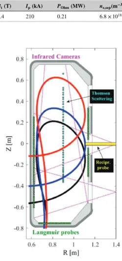
The magnetic configuration of the discharge is shown in Figure 1.

TABLE 1 Main discharge characteristic of shot Tokamak à configuration variable (TCV) #51333

Bt(T) Ip(kA) POhm(MW) ne,sep(m−3)

1.4 210 0.21 6.8 × 1018

FIGURE 1 Magnetic configurations of the Tokamak à configuration variable (TCV) #51333 (by permission from ref.[2]_{). We consider the medium leg}

configuration (blue solid line). HRTS collection points are shown in red

Electron density and temperature profiles are obtained in the outboard mid-plane by high-resolution Thomson scattering. The sampling points are shown in Figure 1. Additionaly, measurements of electron temperature and density are obtained on the divertor targets by Langmuir probes.

In order to estimate the intensity of the turbulent transport in the TCV shot described above, we analyse the experimental data with the transport code SolEdge2D-Eirene.[7]_{As any transport code, SolEdge2D requires providing effective cross-field}

diffusivities to properly account for the turbulent transport. In a “forward” simulation, one provides to the code ad hoc values for the transport coefficients as input and obtains a 2D poloidal map of the plasma density and temperature as output. Experimental mid-plane profiles can thus be compared with simulated ones, and if the match is not satisfactory, one must iterate on the transport coefficient values to improve the agreement between the two. In this paper, we develop a procedure to simplify this iterative process. Instead of providing transport coefficients as input to the code, we directly provide mid-plane profiles of the density and temperature. The code will automatically adjust the transport coefficients so as to match in the end the simulated mid-plane profiles with the experimental ones. More precisely, one uses the proportional–integral feedback loop shown in Figure 2 to correct “on the fly” the transport coefficients while the temporal loop of the code is running.

The gain of the feedback loop𝜏ihas been adjusted to ensure the code stability, while the difference of signals𝜀 is given by

the following formula:

𝜀 = D⊥− D⊥0= 1

𝜏i∫

514 BASCHETTIET AL.

FIGURE 2 Feedback loop used in the code to match simulated mid-plane profiles of density and temperature with the experimental ones. We set the gain and integration time in such a way that the dynamic of the feedback loop is of the order of the parallel plasma characteristic time

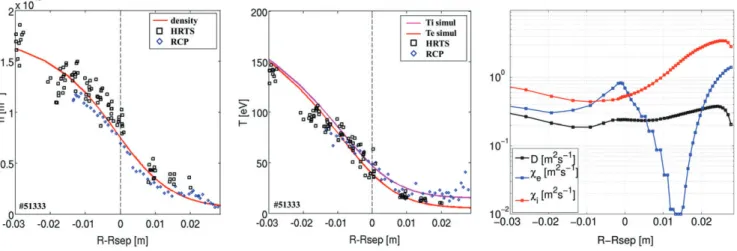
FIGURE 3 Left and middle: Mid-plane profiles of density and temperature (symbol: experimental data, lines: SolEdge2D-Eirene simulation results with feedback procedure) from Ref.[2]_{. Right: Cross-field transport coefficients obtained from the feedback procedure}

where the subscripts “XP” and “simu” stand for “experimental” and “simulation”, respectively. Typically, the time constant associated with the integral correction must be larger than the parallel time𝜏‖= L‖/cs(∼10−5s). The technical details on the

implementation of the procedure are beyond the scope of this paper.

Using this automatic feedback loop procedure, the way of running SolEdge2D is made simple for experimental interpretation. As input of the code, one directly provides experimental measurements of density and temperature in the mid-plane. As output, one still obtains a 2D poloidal map of the density and temperature but additionally gets a 1D profile of the cross-field diffusivities that were ad hoc earlier. The poloidal variation of these coefficients is, however, not taken into account. Since we set the 1D radial profiles of density and temperature at the outer mid-plane, we get 1D radial profiles of diffusivities. The diffusivities are assumed to be homogeneous on each flux surface. Figure 3 shows results of the feedback procedure on the transport coefficients applied to TCV #51333. In this simulation, we consider a pure deuterium plasma. Drift velocities are not taken into account.

Once the code’s free parameters (namely transport coefficients) are set by the feedback procedure, we know that experimental and simulated mid-plane quantities are in rather good agreement.

4 R E D U C T I O N A N D O P T I M I Z A T I O N O F T H E D E G R E E S O F F R E E D O M O F T H E M O D E L

After running SolEdge2D-Eirene as an interpretative tool on TCV #51333, one obtains 2D poloidal maps of density and tem-perature as well as an estimation of the transport coeffcients required to describe the turbulent transport of the discharge in a diffusive fashion. From these data, we propose in this section to optimize the free parameters of our turbulence reduced model. To do so, we apply Equation 4 to the maps of density and temperature computed by SolEdge2D-Eirene for different values of the free parameters of the reduced turbulence model, and compare the diffusivity maps with the transport coefficients obtained from the experiment with the feedback procedure.

As seen in Section 1, we can rewrite Equation 5 as a function of two free parameters:𝛼0and𝜁.

A scan is performed on these two quantities in order to minimize the error between the diffusivities computed with the reduced

𝜅–𝜀 model (D⊥, 𝜅𝜀) and those obtained from the experimental analysis (feedback procedure, D1D_⊥,𝑓𝑏). In Figure 4, the absolute error

𝐸𝑟𝑟(𝛼0, 𝜁) = ‖D⊥,𝜅𝜀− D1D_⊥,fb‖2is parameterized with respect to the two free parameters. The minimum error is found to be for

FIGURE 4 Scan of the relative error𝐸𝑟𝑟(𝛼0, 𝜁) = ||D⊥,𝜅𝜀− D1D⊥,fb||with respect to the free parameters

FIGURE 5 Left: Feedback loopD1D

⊥,fbvs. D⊥, 𝜅𝜀vs. Bohm diffusivity DBohm(the dotted line is the position of the separatrix): flux surface-averaged profiles.

Although usually considered as the standard scaling for diffusion coefficients, and in particular an upper limit, DBohmis actually too small to account for blob

convective transport particularly effective in the SOL region,[8]_{as one can see in the plot. Right: 2D map of diffusivity self-consistently calculated with the} 𝜅−𝜀model. Strange behaviour in the far SOL is due to numerical effects (thresholding of the density)

FIGURE 6 Mid-plane profiles of density and temperature (symbol: experimental data, lines: SolEdge2D-Eirene simulation profiles auto-consistently calculated)

which gives a relative error Errrel,min= 8.6%. Figure 5 shows 2D poloidal maps and flux surface-averaged profile of the

cross-field diffusivities obtained from the reduced turbulent model for the optimum values of the free parameters𝛼0and𝜁. It is

important to stress that the diffusivity is determined for the whole geometrical domain and that the model captures the poloidal asymmetry of the plasma transport due to interchange instability; in particular, the ballooning effect at the low magnetic field side (LFS) is recovered for a divertor geometry as a strong poloidal variation of turbulence transport.[3]

We have implemented the optimized𝜅−𝜀 model into SolEdge2D. The results of this simulation are shown in Figure 6. To run the simulation, ion and electron thermal conductivity have been set proportional to the self-consistently calculated diffusivity. This is an assumption whose validity will not be discussed in this paper but will be investigated in the future work.

516 BASCHETTIET AL.

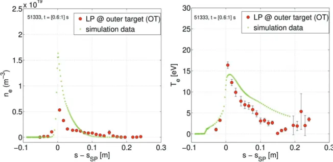
FIGURE 7 Profiles of electron density and temperature at the outer target compared to data collected by the Langmuir probes for shot #51333. Here, s is the curvilinear abscissa along the wall of the vessel, while sSPis the position of the separatrix at the outer target

FIGURE 8 Flow chart representing the loop to infer a self-consistently calculated diffusivity into SolEdge2D. The green path shows the feedback procedure, the red one is the𝜅−𝜀optimization strategy, with𝐸𝑟𝑟(𝛼0, 𝜁) = ||D⊥,𝜅𝜀− D1D⊥,fb||

The outer mid-plane profiles in Figure 6 resulting from the simulation with self-consistently calculated and optimized diffu-sivity show good accordance with the experimental data. A qualitative accordance is also found for the outer target profiles of electron density and temperature, as can be seen from Figure 7. The discrepancy observed for the density target profile is under investigation.

5 C O N C L U S I O N S

A𝜅−𝜀 model has been introduced with the aim of solving the Reynolds averaged Navier–Stokes equations for the SOL plasma. A method to tune the free parameters of the model from experimental data has been presented as well. A summary of this work is sketched in Figure 8. The green line represents the feedback loop between experimental data and SolEdge2D free parameters (anomalous diffusivities). The red line loop represents the strategy consisting of optimizing the𝜅−𝜀 free parameters to recover diffusivity profiles and perform a more consistent comparison between simulation and experimental data, at the outer mid-plane as well as at the outer target. This𝜅−𝜀 procedure allows us to reduce the original number of free parameters and capture the poloidal asymmetries of turbulence, which is a promising first step towards predictive transport models for tokamak plasmas.

A C K N O W L E D G E M E N T S

This work was granted access to the HPC resources of Aix-Marseille Université financed by the project Equip@Meso (ANR-1-EQPX-29-01) of the program “Investissments d’Avenir” supervised by the Agence Nationale pour la Recherche. It has been carried out within the framework of the EUROfusion Consortium and has received funding from the Euratom research and training programme 2014–2018 under grant agreement No. 633053 for the project WP17-ENR-CEA-08. The views and opinions expressed herein do not necessarily reflect those of the European Commission.

R E F E R E N C E S

[2] A. Gallo, N. Fedorczak, S. Elmore, R. Maurizio, H. Reimerdes, C. Theiler, C. K. Tsui, J. A. Boedo, M. Faitsch, H. Bufferand, G. Ciraolo, D. Galassi, P. Ghendrih, M. Valentinuzzi, P. Tamain, the EUROfusion MST1 team, the TCV, Plasma Phys. Control Fusion 2018, 60, 014007.

[3] H. Bufferand, G. Ciraolo, P. Ghendrih, Y. Marandet, J. Bucalossi, C. Colin, N. Fedorczak, D. Galassi, J. Gunn, R. Leybros, E. Serre, P. Tamain, Contrib. Plasma

Phys. 2016, 56(6–8), 555.

[4] K. Miki, P. H. Diamond, N. Fedorczak, Ö. D. Gürcan, M. Malkov, C. Lee, Y. Kosuga, G. Tynan, G. S. Xu, T. Estrada, D. McDonald, L. Schmitz, K. J. Zhao, Nucl.

Fusion 2013, 53, 073044.

[5] F. Hasenbeck, D. Reiser, P. Ghendrih, Y. Marandet, P. Tamain, A. Möller, D. Reiter, Int. Conf. Computational Science, ICCS 2015, 2015, 51(Suppl. C), 1128–1137. [6] X. Garbet, J. Payan, C. Laviron, P. Devynck, S. K. Saha, H. Capes, X. P. Chen, J. P. Coulon, C. Gil, G. R. Harris, T. Hutter, A.-L. Pecquet, A. Truc, P. Hennequin,

F. Gervais, A. Quemeneur, Nucl. Fusion 1992, 32, 2147.

[7] H. Bufferand, G. Ciraolo, Y. Marandet, J. Bucalossi, P. Ghendrih, J. Gunn, N. Mellet, P. Tamain, R. Leybros, N. Fedorczak, F. Schwander, E. Serre, Nucl. Fusion

2015, 55, 053025.