HAL Id: hal-01820698
https://hal.archives-ouvertes.fr/hal-01820698
Submitted on 23 Jun 2018HAL is a multi-disciplinary open access archive for the deposit and dissemination of sci-entific research documents, whether they are pub-lished or not. The documents may come from teaching and research institutions in France or abroad, or from public or private research centers.
L’archive ouverte pluridisciplinaire HAL, est destinée au dépôt et à la diffusion de documents scientifiques de niveau recherche, publiés ou non, émanant des établissements d’enseignement et de recherche français ou étrangers, des laboratoires publics ou privés.
Did Foreign Exchange Holding Influence Growth
Performance During The Global Financial Crisis?
Jean-Pierre Allegret, Audrey Allegret-Sallenave
To cite this version:
Jean-Pierre Allegret, Audrey Allegret-Sallenave. Did Foreign Exchange Holding Influence Growth Performance During The Global Financial Crisis?. The World Economy, Wiley, 2019, 42 (3), pp.680-710. �10.1111/twec.12701�. �hal-01820698�
1
Did Foreign Exchange Holding Influence Growth Performance During The
Global Financial Crisis?
Jean-Pierre Allegret, Université Côte d’Azur, CNRS, GREDEG, jean-pierre.allegret@unice.fr. Audrey Allegret, Univ. of Toulon, Research Fellow EconomiX, UPL, Univ Paris Nanterre, CNRS,
audrey.sallenave@univ-tln.fr.
Abstract
In a context of increased foreign exchange reserves holding from emerging and developing countries, this paper investigates the diminishing return of reserves holding assumption over the most severe phase of the global financial crisis (2008Q1-2010Q4). Relying on a Panel Smooth Transition Regression model, we highlight the differential effect of the accumulation of foreign exchange reserves for a set of financial vulnerabilities variables. Specifically, while reserves accumulation is effective above a critical threshold to cope with vulnerabilities related to the financial channel, we show that it becomes less effective beyond a certain threshold for domestic bank vulnerabilities. Our results are robust to alternative specifications.
Keywords: Financial crisis, Financial vulnerabilities, Panel Smooth Transition Regression model,
Reserves accumulation.
2
1. Introduction
Since the early 2000s, the foreign exchange reserves holding dramatically increased, in particular for emerging and developing countries. As exhibited in Figure 1, while the reserves over GDP ratio has been stable in advanced countries from 1990 to 2000, it increases to about 11% in emerging and developing countries over the same period peaking in 2009 (28.9%). Most importantly, Figure 1 suggests the presence of a major change in the path of reserves holding in these countries at the beginning of the new millennium driven by two events: on the one hand, the East Asian financial crises in 1997-98, and, on the other hand, the capital account liberalization process.
[Insert Figure 1]
An extensive literature analyses the different motives explaining the accumulation of foreign exchange reserves in emerging and developing countries. While the literature distinguishes between the neo-mercantilist approach and the self-insurance one, our paper is based on the latter.1
Specifically, following, among others, Aizenman and Lee (2007), Obstfeld et al. (2010), and Gourinchas and Obstfeld (2012), we link reserves holding to the international financial integration and to the protection of the domestic banking sector against liquidity shocks.2 In line with this
approach, the aim of this paper is to provide an investigation to foreign exchange reserves holding’s capacity -proxied by the ratio reserves minus gold over the monetary aggregate M2- to improve the resilience of economic activity to financial vulnerabilities.
Our paper is related to three strands of the literature. The first one refers to the literature investigating the impact of financial vulnerabilities on the depth and duration of financial crisis. On the external front, Llaudes et al. (2010), Lane and Milesi-Ferretti (2011), and Berkmen et al. (2012) show that countries with higher current account deficits experienced larger output collapses during
1 For an overview of this debate, see Aizenman and Lee (2007). Studying the relationship between real exchange rates
and external asset holdings, Choi and Taylor (2017) attempt to reconcile these two views.
2 An extensive literature suggests that the international financial integration is a major determinant of reserves hoarding.
See, Aizenman and Hutchison (2012), Delatte and Fouquau (2012), Aizenman et al. (2013), and Aizenman and Ito (2014). For a theoretical investigation, see Durdu et al. (2009) who show that financial globalization is a plausible explanation of the hoarding in reserves in emerging countries.
3 the financial crisis. Currency-mismatch and dependence on external funding exert a negative influence on growth performance during the crisis (Llaudes et al, 2010; Calvo et al., 2013; Feldkircher, 2014). On the domestic front, main financial vulnerabilities refer to credit to the private sector indicators (Berkmen et al., 2012; Gourinchas and Obstfeld, 2012; Feldkircher, 2014) and leverage of the financial system, in particular banks (Merrouche and Nier, 2010; Gourinchas and Obstfeld, 2012; Berkmen et al., 2012). The second strand of the related literature concerns the role of foreign reserves holding as a crisis prevention and crisis mitigation.3 An extensive literature
assesses the optimal level of reserves derived from insurance models. Jeanne (2007) and Jeanne and Rancière (2011) present a model of the optimal level of international reserves for a small open economy exposed to loss of access to external credit. Importantly, the sudden stop episodes are associated with falls in domestic output. As the probability of such an episode is a decreasing function of reserves holding, these latter matters as a crisis prevention mechanism and, in turn, reserves hoarding is valuable. On the empirical side, Frankel and Saravelos (2012) claim that reserves accumulation is one of the most robust leading indicators of financial crises. Specifically, they find that higher pre-crisis level of reserves tends to decrease the likelihood of financial crises.4
Our approach is more closely related to international reserves as crisis mitigation. Aizenman and Lee (2007) propose a welfare evaluation of the costs and benefits of reserves accumulation. They analyze a small open economy where financial intermediaries use foreign deposits to invest in long-term projects. As a consequence, the domestic economy is vulnerable to an unexpected liquidity shock. The model shows that hoarding reserves saves liquidation costs, and, then, mitigates the impact of the shock on economic activity. In this insurance model of optimal reserves, Jeanne (2007) shows that foreign exchange interventions can mitigate the depreciation of the domestic currency. In these circumstances, reserves holding reduces output losses of a crisis by lessening the
3 Theoretical models tend to take both motives into account in a single analytical framework. See Jeanne (2007), Jeanne
and Rancière (2011), and Calvo et al. (2013).
4 Using a discrete-choice panel analysis for emerging countries from to 1973 to 2010, Gourinchas and Obstfeld (2012)
find that higher foreign exchange reserves predict a lower probability of a subsequent crisis. See also Catão and Milesi-Ferretti (2014).
4 negative balance sheets effects due to currency mismatches. In a similar way, reserves can mitigate negative impacts of crisis by smoothing domestic absorption in the face of balance of payments shocks. While Blanchard et al. (2010) do not find a relationship between holding a large amount of reserves –proxied through the ratio of reserves to short-term debt- and output loss during the crisis for a sample of 29 emerging countries, many studies find the opposite. For instance, Bussière et al. (2015) assess to what extent pre-crisis foreign reserves accumulation explains economic growth during the crisis. For a sample of 129 developing countries and 32 emerging economies, they find that the accumulation of international reserves during the period preceding the crisis positively contributes to the real GDP growth during the crisis. Dominguez et al. (2012), by investigating the relationship between reserves holding prior to and during the global financial crisis, and real GDP growth in the aftermath of the crisis, get two main findings. First, they show that the larger the reserves holding before the crisis, the higher has been post-crisis growth. Second, depletion of reserves during the crisis tends to improve growth performances in the post-crisis period, but this depletion is conditional to the accumulation of reserve in the pre-crisis period. Finally, the third strand of the literature suggests that reserves accumulation exhibits diminishing returns and hence nonlinear effects. Specifically, while Berkmen et al. (2012) show that countries with higher international reserves experienced smaller growth revisions, the relationship is statistically insignificant. Llaudes et al. (2010) confirm that higher international reserves can help to buffer the impact of the financial crisis.5 But they show that international reserves holding exhibits
diminishing returns. Indeed, at very high levels of reserves holding, the moderating impact on output collapse seems disappear. Alberola et al. (2016) find that large stocks of foreign reserves pay off to mitigate gross capital outflows during periods of systemic financial stress, but, when introducing non-linear effects through quadratic terms, they show that reserves holding exhibits
5 Llaudes et al (2010) consider the ratio reserves over external requirements (sum of the short-term external debt (at
5 decreasing returns. In other words, growing reserves accumulation is less and less effective to reduce capital outflows.
While several contributions suggested the presence of non-linearity using a linear framework -for instance introducing quadratic terms in regressions- this paper deserves more attention to the nonlinear relationship between foreign exchange reserves holding and macroeconomic resilience to a set of financial vulnerabilities indicators for a sample of 40 emerging and developing countries. Focusing on the most intense period of the global financial crisis (2008Q1-2010Q4), we assess whether the negative impact of these vulnerabilities is mitigated beyond a certain level of foreign exchange reserves holding. To the best of our knowledge, the diminishing return hypothesis of reserves holding has not been investigated in a non-linear framework.6 To this end, we apply a
Panel Smooth Transition Regression model developed by Gonzalez et al. (2005) and Fok et al. (2005). This class of model allows to detect asymmetries through threshold effects. Foreign exchange reserves in terms of M2 represent our transition or threshold variable. The PSTR model assumes all parameters to change smoothly between extreme regimes (here we consider two extreme regimes) as a function of the foreign exchange reserves variable.
Our paper contributes to the literature on the crisis mitigation role of reserves in the self-insurance framework by focusing on the diminishing return of reserves holding hypothesis. Our findings highlight the differential effect of the accumulation of reserves by type of vulnerabilities. More precisely, while the holding of reserves above a critical threshold reduces the negative impact on economic activity of financial vulnerabilities linked to the financial channel (e.g. current account balance, international banks lending, VIX index), we show that this accumulation of reserves becomes less effective over this critical threshold for vulnerabilities related to the situation of domestic banks (e.g. currency mismatch, bank leveraging). These findings are especially important for developing countries as reserves accumulation may lead to sub-optimal use of national saving
6 Delatte and Fouquau (2012) uses a non-linear specification -a time-varying panel smooth transition regression model-
6 in a context where many of them suffer from insufficient public investments in infrastructure and education.
The rest of the paper is structured as follows. Section 2 presents countries under study and selected variables. Section 3 introduces our non-linear econometric specifications. Section 4 discusses the main results. Finally, section 5 concludes.
2. Sample and data description
Our country sample includes 40 emerging and developing countries over the period 2008Q1-2010Q4 for the benchmark specification and 1995Q&-2015Q4 for the extended model. This set of countries is decomposed in four sub-samples.7 Two sub-samples distinguish countries according
to their de facto exchange rate regimes. Specifically, using the natural classification by Reinhart and Rogoff (2004), the countries are classified according to the distinction between fixed and floating exchange rates. An interesting feature of this classification is to detect exchange rate regimes changes over a rolling five-year window. This window allows to avoid overestimation of regimes changes exhibiting a short duration. A third sub-sample includes countries adopting inflation targeting framework using the criteria proposed by Freedman and Laxton (2009) and Roger (2009). Lastly, a sub-sample encompasses non-OECD countries. As explained below, we estimate the effectiveness of foreign exchange holding for these sub-samples in order to check the robustness of the findings stemmed from the benchmark model.
The benchmark model includes five indicators of financial vulnerability influencing economic performance during financial crises.8 This relatively small number of variables responds to the need
to build a sufficiently parsimonious model to obtain robust estimators over a very short period. The selected explanatory variables come from the literature on the determinants of financial crises. Three out of five indicators embody the financial channel highlighted in the literature on the global financial crisis. The first indicator is the current account balance in percentage of GDP (ca). This
7 See Appendix A for the list of selected countries. 8 See Appendix B for data description.
7 indicator is especially important to measure to which extend countries are sensitive to sudden stop episodes in capital flows. Indeed, external deficits lead to a dependence on net capital inflows. While the literature tends to consider pre-crisis current account balances9, our paper analyzes the
impact of this variable on economic activity during global financial crisis. This choice allows us to assess the effects of current account adjustment in the aftermath of major interruptions of capital flows.
Our second indicator –the VIX index (vix)- is closely related to the dynamics of capital flows. Indeed, as a measure of the implied volatility of S&P 500 index options, the VIX is also a measure of risk aversion and uncertainty of investors. A recent literature suggests that global factors are a major determinant of waves of capital flows that explain their synchronicity at a worldwide level and the formation of a global financial cycle (Rey, 2013). Specifically, increase in global uncertainty and risk aversion, e.g. a rise in VIX, is associated with stops and retrenchments. Such relationship is observed for both gross capital flows (Forbes and Warnock, 2012) and net capital inflows (Ghosh et al., 2014). In addition, as stressed by Shin (2016), the VIX index has been until recently a barometer of the appetite for leverage of the banks. In other words, VIX has exerted a significant influence on international credit flows through banking leverage.
The last external financial vulnerability indicator is the international claims of BIS-reporting banks in percentage of borrowers’ GDP (bis inter). As we use consolidated statistics, international claims are defined as “the sum of cross-border claims in any currency and local claims of foreign affiliates denominated in non-local currencies”.10 In other words, we exclude from our estimations local
claims in local currencies in order to better isolate external vulnerabilities and the role of international reserves.11 This variable is important for two main reasons. On the one hand, it allows
to take into account the critical role of banking flows in international capital movements until
9 See, for instance, Lane and Milesi-Ferretti (2011), Berkmen and al. (2012), and Adler and Tovar (2012). These papers
find that current account deficits amplify the negative effects of external financial shocks on domestic economies.
10 Guidelines for reporting BIS international banking statistics.
See http://www.bis.org/statistics/bankstatsguide.htm.
8 2010.12 On the other hand, in many emerging and developing countries, the expansion of domestic
credit has been fueled by international banking credit. From this perspective, the major retrenchment in the international banking activity in the aftermath of the collapse of the Lehman Brothers in September 2008 has been a serious shock for many emerging and developing countries.13
Our last two vulnerability indicators are more closely related to liquidity tensions for the banking system during periods of financial stress. As a proxy of liability dollarization, we include in our set of explanatory variables the ratio of foreign liabilities in the domestic financial sector relative to money stocks (currency mismatch) (Levy-Yeyati et al., 2010). An extensive literature stresses that the higher the domestic liability dollarization, the higher is the output loss in the aftermath of exchange rate depreciation.14 As a result, the presence of currency mismatch constraints the ability of
monetary policy to respond to external shocks. Specifically, fear of floating due to the currency mismatch leads to pro-cyclical monetary policy responses.15
Lastly, in order to grasp the exposition of banks to wholesale funding, we consider the ratio of bank credit to bank deposits (credit deposit). Merrouche and Nier (2010) show that this bank leverage ratio dramatically increased in the run-up to the Nordic (1991) and Asian (1997) crises. Distinguishing between core liabilities (retail deposits) and non-core liabilities (other funding sources including wholesale market), Hahm et al. (2013) find that a large stock of non-core liabilities increases the vulnerability to crises.16
To test the robustness check of our results, we add two variables. On the one hand, following Rodrik (2006), we introduce the ratio short-term external debt to GDP to see to what extent
12 This period corresponds to the first phase of global liquidity according to Shin (2013).
13 Berkmen et al. (2012) and Feldkircher (2014) find that countries borrowing more from advanced economies’ banks
have been hit harder during the global financial crisis.
14 For the Latin American countries’ experience, see Cavallo and Izquierdo (2009).
15 For a sample of 21 industrial countries and 47 developing countries over the period 1960-2009, Vegh and Vulletin
(2012) show that the higher the fear of floating, the more pro-cyclical monetary policy. For a sample of 10 emerging European economies over the period 1995-2010, Allegret et al. (2014) find that countries with high currency mismatch exhibit both a fear of floating and a fear of losing international reserves.
9 holding foreign reserves lessens this external vulnerability to sudden stop in capital inflows.17 On
the other hand, we consider the fiscal balance in terms of GDP as an additional policy control variable.18
As we are especially interested by the nonlinear effect of reserves holding to mitigate the impact of financial vulnerabilities on economic activity, we select as threshold variable the ratio foreign exchange minus gold reserves19 over the monetary aggregate M2 (forex). This choice is in line with
the financial stability approach -based on the “double drains” assumption- proposed by Obstfeld et al. (2010).
Figure 2 portrays the evolution of this ratio from 1995Q1 to 2015Q4 for all studied countries (left part) and our subsamples (right hand). Ratios are weighted by the share of each country in the world stock of reserves minus gold. The shaded area corresponds to the Global financial crisis (2008Q1-2010Q4) which is the focus of our analysis. As in Figure 1, the striking lesson drawn from this figure in is the dramatic increase in the ratio over the 2000 decade. As expected, the right part of the figure shows that this trend is largely driven by non-OECD countries and economies under peg exchange rate regimes.
[Insert Figure 2] 3. Methodology
In this section, we proceed in two steps: after considering a linear specification, we introduce threshold effects using a non-linear specification based on a Panel Smooth Threshold Regression (PSTR) model.
17 Rodrik (2006) investigates different ways to increase liquidity countries understood as higher net levels of liquid
foreign assets. He suggests three strategies: creating a collateralized credit facility, increasing foreign exchange reserves, and reducing short-term debt. We tried to test the last strategy by considering the short-term external debt in percentage of GDP as a transition variable. However, tests carried out led us to reject the hypothesis of non-linearity. Results are available from the authors upon request.
18 Specifically, we use the ratio General government primary net lending/borrowing to GDP. We thank the anonymous
referee to suggest assessing to what extent our results are robust when we consider the impact of fiscal policy on economic activity.
19 We have also considered the foreign exchange reserves as the transition variable and this does not change
10
The linear specification
To put forward the interest of a nonlinear specification, we estimate in this section a linear version of our model where we include a quadratic term of the foreign exchange reserves. We expect an opposite sign of the forex when considering the quadratic term coefficient, meaning that the foreign exchange reserves holding have a potential nonlinear effect. We proceed to two estimations, the first over the period 2008Q1-2010Q4, namely our benchmark model, and the second over the extended period that goes from 1995Q1 to 2015Q4.
For each of them we face to cross sectional and temporal dependencies that can lead to biased statistical inference. Then, we ensure the validity of the statistical results by adjusting the standard errors of the coefficient estimates of our regression for possible dependence in the residuals. To this aim, we then implement the Driscoll and Kraay’s (1998) covariance matrix estimator for use of our fixed effect regressions. This estimator can be used for unbalanced panels and has small sample properties that are significantly better than those of the alternative covariance estimator when cross-sectional dependence is present.
As a preliminary step, we test the presence of cross-sectional dependencies, performing the Pesaran’s (2004) CD test that can be either applied to models including small or large N and T. The null hypothesis stands for zero dependence across the panel units. This test is based upon an average of all pair-wise correlations of the ordinary least squares residuals from the individual regressions.
We estimate the following model:
ℎ = + + + + + +
! + " (1)
where = 1, … , & represents each cross-section, = 1, … , ' refers to the time period. and are respectively the intercepts and the slope coefficients that are allowed to vary across the panel members. The endogenous variable, standing for the economic activity, is the real GDP gross rate
11 (gdp growth). In (1), ca, bis inter, vix, currency, and credit deposit are our financial vulnerabilities defined above.
The cross-sectional dependencies test is defined as:
() = *,(,. )+ 0∑,.5 ∑,45 6 2347 → &(0,1) (2)
where 234 is the sample estimate of the pairwise correlation of the OLS estimated residuals :̂ of equation (1). 234 is expressed as:
234= 234 = ∑ <=>?<=@? A ?BC 0∑A <=>?D ?BC 7C/DF∑A?BC <=@?DGC/D (3)
Results of the cross-sectional dependencies test displayed in Table 1a and 1b indicate that the null hypothesis of cross-section independence is strongly rejected at the standard level of 5%. According to these results, equation (1) must be estimated with Driscoll-Kraay standard errors since they are robust to cross section dependence.
[Insert Table 1a] [Insert Table 1b]
Using a linear framework, we aim at identifying the existence of nonlinearity in the impact played by the foreign exchange reserves on economic growth for each of our samples. This will give us a first basis for further comparatives when estimating a nonlinear model. We then introduce in equation (1) a quadratic term on the forex variable in order to identify a possible nonlinear effect on the gdp growth variable.
The linear estimated model is the following:
ℎ = + + + + + +
! + H (! )² + " (4)
In the benchmark model and the extended estimation, and for each of our sub-samples, the nonlinearity in the forex-growth nexus is observed as we obtain a negative linear effect and a positive quadratic term (Table 2a and 2b). This result leads us to investigate in a nonlinear
12 framework the financial crisis mitigation role of reserves holding when countries have significant financial vulnerability.
[Insert Table 2a] [Insert Table 2b]
Dealing with nonlinearities: The Panel Smooth Transition Regression
As we have detected a potential non-linear relationship between foreign exchange reserves and growth, we now turn to the estimation of a Panel Smooth Threshold Regression (PSTR) model introduced by Gonzalez et al. (2005) and Fok et al. (2005).
We consider the following two-regime PSTR model:
= : + JK + K (L ; N, ) + " (5)
where: is a vector of fixed individual effects, = J, … , O, K = (K , … , KO) is the matrix of P explanatory variables, Q denotes the threshold variable, and the error " is assumed to be i.i.d (0,RS). The transition function T(Q ; N, ) is a continuous and bounded function between 0 and 1 of the threshold variable Q .
Gonzalez et al. (2005) consider, following Granger and Terasvirta (1993) for time series STAR models, the following logistic specification for the transition function:
(L ; N, ) = [1 + exp (−N ∏ (L −\[5 [)]. (6)
with ≤ ≤ \ and N > 0. [= ( , … , \)` denotes a m-dimensional vector of location parameters, i.e. the critical levels separating two continuous regimes and N determines the slope of the transition function and stands for the smoothness of the transition across regimes. When m = 1 and N → ∞, the transition function T(. ) becomes indicator functions and the model reduces to a simple Panel Transition Regression model introduced by Hansen (1999). On the contrary, when N → 0, T(. ) becomes constant and the model collapses to a simple panel linear regression model with fixed effects. Between the two extreme cases, i.e. m > 1 and N → ∞, the number of identical regimes remains two, but the function switches between zero and one at , … , \.
13 The value of m affects the regime-switching behavior. In this paper, we consider a model with one transition function and m = 1. It implies a monotonic change of the coefficient J to J+ as L increases.
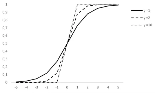
Appendix C displays an analysis of the slope parameter according to the various values of N. As the procedure provides for the estimation all the parameters of interest in the model, including any N and , a priori identification of the regimes is not required.
A possible generalization of the PSTR model is the general additive PSTR model:
= : + J` + ∑c45 4` 4Fd(4); N4; 4G + : (7)
where the transition function is type of (2) and r denotes the number of regimes.
Before estimating the PSTR model, the first step is to test the presence of nonlinearity. More specifically, as the PSTR is not identified if the data-generating process is linear, linearity test is necessary to avoid the estimation of unidentified models. Here, we follow Lüükkonen et al. (1988) as they allow us to test for the number of transition functions in the model. We first test the null of a linear specification, corresponding to r = 0, against a non-linear one, corresponding to r = 1. The rejection of the null leads us to test the possibility of the presence of two thresholds (r = 2). The procedure continues until we reject any additional threshold. Results20 (see Table 3) clearly
indicate that we fail to retain the linearity hypothesis, whatever the sub-sample under consideration, and the number of thresholds is established to one. This test indicates that a two-regime model yields a sufficient characterization of the nonlinearity in the data. We have then strong evidence on nonlinearity in the relationship between forex and growth. We can now turn to the estimation of the PSTR model.
[Insert Table 3]
20 Non linearity tests for the extended estimation give similar results as we reject the null of linearity for each of our
14
4. Results
In a first step, we consider results from the baseline specification. In a second step, we perform several robustness tests.
Results of the baseline model
Table 4 exhibits the results for the whole sample. The last line gives the threshold value (39.5%) for our variable of interest, i.e. the ratio foreign reserves minus gold over M2.
The
β
coefficients for the current account balances in percentage of GDP are negative in the first and second regime. This finding is in line with the literature on sharp current account reversals in the aftermath of sudden stop episodes (Milesi-Ferretti and Razin, 2000; Edwards, 2007). Results show thatβ coefficients in the second regime is consistently below its value in the first one
suggesting that official reserves accumulation is beneficial to lessen the negative impact of current account adjustments on economic activity.[Insert Table 4]
As expected, VIX index coefficients in regimes 1 and 2 are negative, implying that an increase in risk aversion exerts a negative influence on GDP. Such influence rests on the fact that this global factor is one of the main determinants of international capital flows. However, in line with the self-insurance motive, we find that holding reserves is effective to protect domestic economies against international financial shocks as β coefficients in regime 1 is higher than in regime 2.
The dramatic retrenchment of international banks has exerted a negative influence on GDP growth in emerging and developing countries. This influence in part results from the relationship between international bank flows and domestic credit expansion, and, in turn, growth performance. Our results confirm such presumption as
β coefficients are negative. Importantly, we show that
β
coefficients in regime 2 is lower than in the first regime. In other words, holding higher reserves mitigates the negative impact of disruption of international credit flows.15 Overall, our findings suggest that increasing the stock of international reserves allows domestic authorities to mitigate the negative impacts of shocks transmitted through the financial channel. Indeed, β coefficients in the second regime are consistently lower than their values in the first one. Importantly, results in Table 4 suggest that vulnerability indicators related to liquidity stress in the banking sector lead to different conclusions about the effectiveness of reserves accumulation. The ratio of foreign liabilities in the domestic financial sector relative to money stocks represents our proxy to measure the extent of the currency mismatch. As stressed above, this vulnerability indicator is important to consider as financial crises tend to lead to sizable currency depreciations.21
Specifically, high levels of currency mismatch are associated with contractionary effects of depreciations instead of expansionary impact as in the traditional Mundell-Fleming model. This contractionary effect rests on the negative balance sheet effect owing to liabilities dollarization (Frankel, 2005). Our estimations in Table 4 confirm this negative effect and show that, when significant,
β
coefficients in both regimes are negative. Results suggest that reserves accumulation is ineffective to lessen the negative impact of currency mismatch on economic performance. Indeed, β coefficients in the second regime is consistently higher than β coefficients in the first one.The last indicator -the credit to deposit ratio- is a proxy for the dependence of domestic banks on less stable funding than retail deposits. This indicator gives also an approximation for the exposition of banks to a sudden freeze of wholesale funding markets as experienced in the aftermath of the Lehman Brother collapse. In line with the literature stressing that higher credit to deposit ratio increase the vulnerability of banks to financial shocks, our results show that
β
coefficients in both regimes are negative. Higher ratios lead to lower GDP growth. As for the foreign liabilities in the domestic financial sector relative to money stocks ratio, we see that reserves accumulation is ineffective to lessen this negative impact.
16 These two last findings are especially important with regard the self-insurance motive. Aizenman and Lee (2007) show that vulnerability to liquidity shocks implies a complementarity between demand for reserves and demand for deposits. Since 2000, some countries experienced episodes in which central banks used their international reserves to provide foreign liquidity to the banking sector and, sometimes, specific sectors. For instance, in 2002, Brazilian central banklent its reserves to the export sector through commercial banks; in the aftermath of the Argentine crisis, the Central Bank of Uruguay used its reserves to face the withdrawal of dollar-denominated deposits from the domestic banking system.22 In 1997, the South Korean central bank employed its foreign reserves
to make loans to commercial banks in order to provide them foreign currency refinancing. However, our results about the currency mismatch and the credits to deposits ratio suggest a negative assessment concerning the effectiveness of reserves accumulation.
Robustness checks
This section discusses the robustness of our results to different model specifications. In a first step, we examine whether our baseline results are sensitive to the monetary regimes -exchange rate regimes and inflation targeting- and to the level of financial development.23 In a second robustness
investigation, the benchmark model is estimated over a longer period (1995Q1-2015Q4) allowing us to consider both the Asian and Global financial crises, and its aftermath. This period is used to assess the impact of fiscal policy on our results. In a last step, we consider the short-term external debt in percentage of GDP as an alternative external vulnerability variable.
What roles for the monetary regimes and the level of financial development?
Distinguishing studied countries according to their exchange rate regimes is relevant to investigate to what extend the stabilizing impact attributed to reserves holding is due to the floating classification countries. Indeed, an extensive literature shows that more flexible exchange rates help to buffer shocks during crises (IMF, 2010; Adler and Tovar, 2012). In a similar way, we check the
22 According to Jeanne (2007), such intervention has led to a decline in domestic absorption significantly smaller than
the shock to the capital account. For the Brazilian experience, see Calvo (2006).
17 robustness of our results by investigating countries with an inflation targeting framework. As suggested, for instance by de Carvalho Fillo (2011) and Coulibaly (2012), inflation targeters tend to outperform other countries during the global financial crisis. As a proxy of macro-stability and rules-based macroeconomic policy, this monetary regime allowed authorities to adopt countercyclical monetary policy during the crisis. The non-OECD sub-sample may be particularly sensitive to financial vulnerabilities insofar as their financial systems tend to be less robust.
Threshold values are relatively close for the full sample (Table 4): peggers and non-OECD countries, in a range of 39-40%, while they are higher for floaters and inflation targeting economies (54.33% and 57.50% respectively).24
Figures E1 to E4 in Appendix E give an overview of the vulnerability indicators for each sub-sample. Over the period 2008Q1-2010Q4, countries under peg exchange rate regimes exhibit the worst situation as both indicators related to the financial channel -i.e. the current account balance and the international claims of BIS-reporting banks- and indicators concerning liquidity tensions for the banking system -the levels of currency mismatch and leverage- are higher than in other sub-samples. Conversely, except for the current account deficit, non-OECD countries appear to be the less vulnerable.
Regarding the findings of the PSTR for the financial vulnerability variables, the most important lesson is that our results for the sub-samples confirm those obtained with the full sample. The current account variable exhibits negative β coefficients whatever the considered sub-sample. In other words, reducing current account deficits during financial crises is costly in terms of economic activity. As for the baseline model, results show that β coefficients in the second regime are consistently below the β coefficients in the first regime except for the inflation targeting sub-sample. According to the literature and confirming the previous results of the full sample model, the coefficients of bis inter and vix are negative. For each variable, we find a lower coefficient in the
24 About 34% of the observations are above the threshold in the full sample; this share amounting to 40%, 37%, 15%,
18 second regime compared to the first one. Interestingly, even countries with higher degree of capital account openness, i-e, float and inflation targeting countries –using either the Chinn and Ito index- or with less capital control measures (Fernandez et al, 2016) can lessen the impacts of the VIX increase on their economic activity. As in the full sample model, we find that reserves accumulation is ineffective to lessen the negative influence of the credit to deposit ratio on economic activity. Interesting differences with the full sample model can be highlighted with the currency variable. On the one hand, for the peg sub-sample, we find that holding reserves above the critical threshold improves the resilience of economic activity to currency mismatch. Such result is particularly remarkable insofar as peggers exhibit the higher ratios. On the other hand, unlike the other sub-samples, we find that the currency mismatch coefficients are positive in both regimes for floating exchange rate countries. This result can be explained by the fact that these countries tend to have a lower level of currency mismatch.25
Are reserves accumulation effective to face financial vulnerabilities over a longer period?
During the period 1995-2015, the global economy has experienced various events exerting influence on the financial vulnerability of economies. In a first sub-period, from 1995 to 2001, many emerging economies have been hit by currency and banking crises followed by more volatile international capital flows and higher risk premia. From this standpoint, the Asian and Russian crises (1997-1998) played a key role. The second sub-period refers to the so-called Great moderation (2002-2007) in the aftermath of the Dotcom bubble collapse. The U.S. accommodative monetary policy has led to a period of very low risk premia (see for instance the behavior of the VIX index in figure E5) fueling the accumulation of financial disequilibria, in particular in the banking sector (See figures E3 and E4). The post-global financial crisis sub-period is characterized by two main events. On the one hand, the European sovereign debt crisis (2010-2012) has led to a rise in global
25 Note that while the degree of currency mismatch is the lowest in non-OECD countries, it exerts a negative influence
on economic activity in both regimes. Accumulating foreign reserves do not improve the ability of authorities to cope with this financial vulnerability. The low level of financial development in many non-OECD countries may explain such result.
19 risk aversion (See figure E5) with adverse consequences for equity returns. In addition, countries with trade and / or financial ties suffer particularly from this crisis. On the other hand, in mid-2013, the U.S. Federal Reserves communicated on the tapering unconventional monetary policies in the near future. Therefore, emerging markets experienced financial turbulence -capital outflows, exchange rate depreciation, foreign reserves losses- and their domestic economic activity slowed. Tables D5-D8 (columns 1-2) in Appendix D show the results over the period 1995Q1-2015Q4.26
For all samples, we find lower threshold values than in the baseline model. Such a result can be explained by the fact that our period includes both tranquil and turbulent sub-periods. Consequently, relative to the period 2008Q1-2010Q4, the level of financial vulnerability is lower. Specifically, figures E1-E4 show clearly that our vulnerability indicators reached their peak values around two periods characterized by financial crises: 1995-1999 and 2008-2010. In addition, the distribution of observations suggests that pegger and non-OECD countries have accumulated excessive reserves as more than 70% of these observations are above their respective threshold values.27
Tables D5-D8 (columns 1-2) confirm previous findings about the effectiveness of reserves holding to cope with financial vulnerability. We can thus consider that our estimates are robust to the inclusion of several shocks affecting the world economy. However, an important exception is the leverage ratio variable (credit deposit). While we find that reserves accumulation is ineffective to lessen the negative effect of this vulnerability for the period 2008Q1-2010Q4, we get the opposite for the period 1995Q1-2015Q4. This finding suggests that for lower leverage ratio, reserves holding is effective to face this banking vulnerability.28
26 As many countries adopted an inflation targeting regime after 2000, we do not run estimates for this period. 27 The distribution of observations above the respective threshold values is the following: 59% for the full sample,
72% for the peg sub-sample, 73% for non-OECD members, and 34% for the float sub-sample.
28 On average, all sub-samples have lower leverage ratios over the period 1995-2015 relative to 2008-2010. See figure
20
Are the results robust to the introduction of the fiscal variable?
Tables D5-D8 (columns 3-4) in Appendix D present our results after adding a fiscal variable as control variable. We aim at examining to what extent our main findings on the effectiveness of reserves accumulation are still valid when we include in the model this policy variable. Three lessons are drawn from these new estimates. First, considering the impact of fiscal consolidation, our results suggest a negative impact of activity for the full sample and all sub-samples. As expected, reserves holding is ineffective to lessen this effect.
Second, all estimates show higher threshold values leading us to conclude to a destabilizing impact of fiscal policy on financial stability. Importantly, the reversal of the results for the current account variable highlights this finding. Specifically, after introducing the fiscal variable, we see that reserves holding is ineffective to dampen damages due to current account adjustments.
Third, the other variable exhibiting some changes is the currency mismatch ratio (currency). Except for the peg sub-sample, we find that the effectiveness of reserves holding to cope with this vulnerability improves suggesting a complementarity between fiscal policy and reserves accumulation for variables related to banking vulnerability.
However, it is important to be cautious in interpreting these results. On the one hand, our estimates do not capture changes in fiscal policy adopted in emerging and developing countries over the studied period. Indeed, as stressed among other by Frankel et al. (2013), an increasing number of these countries improved their fiscal effectiveness by adopting counter-cyclical policy over the 2000 decade. On the other hand, our fiscal variable does not allow us to estimate fiscal multipliers. As a consequence, our model may underestimate the macroeconomic impact of fiscal policy.
Which lessons drawn from the introduction to the external short-term debt?
Tables D9-D13 in Appendix D show the results of the model including external short-term debt as a percentage of GDP as vulnerability indicator. Columns 1-2 refer to the 2008Q1-2010Q4 period and columns 3-4 to the 1995Q1-2015Q4 one. As the variable bis inter has a high correlation coefficient with external debt, we drop the former in the new estimates.
21 First of all, whatever the periods, the external short-term debt exerts a negative influence on GDP changes. However, in line with Rodrik (2006), we find that reserves holding mitigates this negative impact. Second, for the two periods, our results -except to a lesser extent for the leverage ratio over the period 2008Q1-2010Q4- are qualitatively similar to the model without debt.
5. Conclusion
Emerging and developing countries have accumulated a huge stock of foreign exchange reserves, in particular after 2000. The self-insurance motive literature has stressed the mitigation role of reserves to face financial crises. Specifically, holding reserves allows authorities to limit both exchange rate depreciations and contraction in domestic absorption following a sudden stop episode. In this paper, we investigate the effectiveness of reserves accumulation by focusing on the diminishing return hypothesis. We estimate a nonlinear Panel Smooth Transition Regression for a panel of emerging and developing countries over the crisis period spanning from 2008Q1 to 2010Q4. Our results partially support this hypothesis insofar as we show that reserves accumulation above a critical threshold does not dampen the negative effects of bank financial vulnerabilities. However, our findings suggest that reserves holding is effective to respond to macro-financial vulnerabilities. These findings are robust to alternative specifications.
These results support the complementarity between different tools to manage the potential destabilizing effects of the international financial integration. In the context of this paper, macroprudential measures -such as leverage cap and limits applied to the foreign exchange-denominated liabilities of the banking sector- and the accumulation of foreign reserves. Such complementary is particularly important for many developing countries which suffer from public investment shortage in infrastructure and education. Indeed, reserves accumulation has an opportunity cost, and this latter is particularly high when reserves holding is not effective to protect the domestic economy against financial vulnerabilities.
22
6. References
Adler, G., and Tovar, C.E., 2012. Riding global financial waves: the economic impact of global financial shocks on emerging market economies. IMF Working Paper. WP/12/188. July.
Aizenman, J., and Hutchison, M., 2012. Exchange market pressure and absorption by international reserves: emerging markets and fear of reserves loss during the 2008-09 crisis. Journal of International Money and Finance. 3: 1076-1091.
Aizenman, J., and Ito, H., 2014. Living with the trilemma constraint: Relative trilemma policy divergence, crises, and output losses for developing countries. Journal of International Money and Finance. 49: 28-51.
Aizenman, J., and Lee, J., 2007. International reserves: precautionary versus mercantilist views, theory and evidence. Open Economies Review. 18:191–214.
Aizenman, J., Chinn, M.D., and Ito, H., 2013. The “impossible trinity” hypothesis in an era of global imbalances: measurement and testing. Review of International Economics. 21: 447–458. Alberola, E, Erceb, A., and Serena, J.M., 2016. International reserves and gross capital flows dynamics. Journal of International Money and Finance. 60: 151-171.
Allegret, J.P., Beker-Pucar, E., Gimet, C., and Josifidis, K., 2014. Macroeconomic policy responses to financial crises in emerging European economies. Economic Modelling. 36: 577–591.
Berkmen, S.P., Gelos, G., Rennhack, R., and Walsh, J.P., 2012. The global financial crisis: explaining cross-country differences in the output impact. Journal of International Money and Finance. 31: 42-59.
Blanchard, O.J., Das, M., and Faruqee, H., 2010. The initial impact of the crisis on emerging market countries. Brookings Papers on Economic Activity. 41: 263–323.
Bussière, M., Cheng, G., Chinn, M.D., and Lisack, N., 2015. For a few dollars more: reserves and growth in times of crises. Journal of International Money and Finance. 52: 127–145.
Calvo, G.A., 2006. Monetary policy challenges in emerging markets: sudden stop, liability dollarization, and lender of last resort. NBER Working Paper. N°12788. December.
Calvo, G.A., Izquierdo, A., and Loo-Kung, R., 2013. Optimal holdings of international reserves: self-insurance against sudden stops. Monetaria, Centro de Estudios Monetarios Latinoamericanos. 1: 1-35.
Catão, L.A.V., and Milesi-Ferretti, G.M., 2014. External liabilities and crises. Journal of International Economics. 94: 18-32.
Cavallo, E., and Izquierdo, A., 2009. Policy responses to sudden stops: a comparative analysis. In Cavallo, E., Izquierdo, A. (Eds.). Dealing with an international credit crunch, policy responses to sudden stops in Latin America. Inter-American Development Bank. Washington D.C. 1–22. Choi, W.J., and Taylor, A.M., 2017. Precaution versus mercantilism: reserves accumulation, capital controls, and the real exchange rate. NBER Working Paper. N°23341. April.
Coulibaly, B., 2012. Monetary policy in emerging market economies: what lessons from the global financial crisis? Board of Governors of the Federal Reserve System. International Finance Discussion Papers. No. 1042. February.
de Carvalho Filho, I., 2011. 28 months later: how inflation targeters outperformed their peers in the great recession. The B.E. Journal of Macroeconomics. Berkeley Electronic Press. vol. 11(1). article 22.
23 Delatte, A.L., and Fouquau, J., 2012. What drove the massive hoarding of international reserves in emerging economies? A time-varying approach. Review of International Economics. 20:164–176. Dominguez, K.M.E., Hashimoto, Y., and Ito, T., 2012. International reserves and the global financial crisis. Journal of International Economics. 88: 388-406.
Driscoll, J.C., and Kraay, A.C., 1998. Consistent covariance matrix estimation with spatially dependent panel data. Review of Economics and Statistics. 80: 549-560.
Durdu, C.B., Mendoza, E.G., and Terrones, M.E., 2009. Precautionary demand for foreign assets in Sudden Stop economies: An assessment of the New Mercantilism. Journal of Development Economics. 89: 194-209.
Edwards, S., 2007. Capital controls, sudden stops, and current account reversals, in Edwards S. (Dd.), Capital Controls and Capital Flows in Emerging Economies, University of Chicago Press: 73-120.
Feldkircher, M., 2014. The determinants of vulnerability to the global financial crisis 2008 to 2009: credit growth and other sources of risk. Journal of International Money and Finance. 43: 19-49. Fernández, A., Klein, M.W., Rebucci, A., Schindler, M., and Uribe, M., 2016. Capital control measures: a new dataset. IMF Economic Review. 64: 548-574.
Fok, D., van Dijk, D., and Franses, P., 2005. A multi-level Panel STAR model for US manufacturing sectors. Journal of Applied Econometrics. 20: 811–827.
Forbes, K.J., and Warnock, F.E., 2012. Capital flow waves: Surges, stops, flight, and retrenchment. Journal of International Economics. 88: 235–251.
Frankel, J.A., 2005. Mundell-Fleming lecture: Contractionary currency crashes in developing countries. IMF Staff Papers. 52: 149-192.
Frankel J.A., Végh C.A., and Vuletin G. (2013). Journal of Development Economics. 100: 32-47. Frankel, J.A., and Saravelos, G., 2012. Can leading indicators assess country vulnerability? Evidence from the 2008–09 global financial crisis. Journal of International Economics. 87: 216-231.
Freedman, C., and Laxton, D., 2009. Why inflation targeting? IMF Working Paper. WP/09/86. April.
Ghosh, A.R., Qureshi, M.S., Kim, J.I., and Zalduendo, J., 2014. Surges. Journal of International Economics. 92: 266-285.
Goldstein, M., and Turner, P., 2004. Controlling currency mismatches in emerging markets. Institute for International Economics. Washington D.C.
González, A., Teräsvirta, T., and van Dijk, D., 2005. Panel Smooth Transition Regression model. SSE/EFI Working Paper Series in Economics and Finance 604. Stockholm School of Economics. Granger, C., and Teräsvirta, T., 1993. Modelling nonlinear economic relationship. Oxford University Press. USA.
Gourinchas, P.O., and Obstfeld, M., 2012. Stories of the twentieth century for the twenty-first. American Economic Journal: Macroeconomics. 4:226-265.
Hahm, J.H., Shin, H.S., and Shin, K., 2013. Noncore bank liabilities and financial vulnerability. Journal of Money. Credit and Banking. 45: 3-36.
Hansen, B.E., 1999. Threshold effects in non-dynamic panels: estimation, testing, and inference. Journal of Econometrics 93 (2). pp. 345–368.
24 International Monetary Fund, 2010. How did emerging markets cope in the crisis? Strategy, Policy, and Review Department. June. Washington D.C.
Jeanne, O., 2007. International reserves in emerging market countries: too much of a good thing? Brookings Papers on Economic Activity. 1: 1-80.
Jeanne, O., and Rancière, R., 2011. The optimal level of international reserves for emerging market countries: a new formula and some applications. The Economic Journal. 121: 905–930.
Lane, P.R., and Milesi-Ferretti, G.M., 2011. The cross-country incidence of the global crisis. IMF Economic Review. 59: 77-110.
Levy Yeyati, E., Sturzenegger, F., and Reggio, I., 2010. On the endogeneity of exchange rate regimes. European Economic Review. 54: 659–677.
Llaudes, R., Salma, F., and Chivakul, M., 2010. The impact of the great recession on emerging markets. IMF Working Paper. WP/10/237. October.
Lüükkonen, R., Saikkonen, P., and Teräsvirta, T., 1988. Testing linearity against smooth transition autoregressive models. Biometrika 75(3) . 491-499.
Merrouche, O., and Nier, E., 2010. What caused the global financial crisis? Evidence on the drivers of financial imbalances 1999–2007. IMF Working Paper. WP/10/265. December.
Milesi-Ferretti, G.M., and Razin, A., 2000. Current account reversals and currency crises: empirical Regularities, in Krugman P.R. (Ed), Currency crises, University of Chicago Press, 285-323.
Obstfeld, M., Shambaugh, J.C., and Taylor, A.M., 2010. Financial stability, the trilemma, and international reserves. American Economic Journal: Macroeconomics. 2: 57-94.
Pesaran, M.H., 2004. General diagnostic tests for cross section dependence in panels. University of Cambridge, Faculty of Economics. Cambridge Working Papers in Economics. No. 0435. Reinhart, C.M., and Rogoff, K.S., 2004. The modern history of exchange rate arrangements: a reinterpretation. The Quarterly Journal of Economics. 119: 1-48.
Rey, H., 2013. Dilemma not trilemma: the global financial cycle and monetary policy independence, in Global Dimensions of Unconventional Monetary Policy, Economic Policy Symposium Proceedings, Federal Reserve Bank of Kansas City, 285-333.
Rodrik, Dani, 2006, The social cost of foreign exchange reserves. International Economic Journal, 20: 253-266.
Roger, S., 2009. Inflation targeting at 20: achievements and challenges. IMF Working Paper. WP/09/236. October.
Shin, H.S., 2013. The second phase of global liquidity and its impact of emerging economies. Keynote address at the Federal Reserve Bank of San Francisco Asia Economic Policy Conference. November 3-5.
Shin, H.S., 2016. The bank/capital markets nexus goes global. Speech at the London School of Economics and Political Science. November 15.
Vegh, C.A., and Vuletin, G., 2012. Overcoming the fear of free falling: monetary policy graduation in emerging markets. NBER Working Paper Series. N°18175. June.
25
Tables
Table 1a: Pesaran's test of cross sectional independence 2008Q1-2010Q4
Full sample
Float Peg Inflation targeting
Non-OECD CD test 29.659 (0.00) 20.913 (0.00) 8.748 (0.00) 17.936 (0.00) 19.746 (0.00) Average correlation coefficient 0.388 0.475 0.325 0.496 0.368
Notes: CD stands for Pesaran's test of cross sectional independence. p-value are given between brackets. We report the average and absolute correlation coefficients across N x (N‐1) pairs of correlation.
Table 1b: Pesaran's test of cross sectional independence 1995Q1-2010Q4
Full sample Float Peg Non-OECD
CD test 35.740 (0.00) 24.921 (0.00) 14.176 (0.00) 24.928 (0.00)
Average correlation coefficient 0.206 0.234 0.214 0.207
Notes: CD stands for Pesaran's test of cross sectional independence. p-value are given between brackets. We report the average and absolute correlation coefficients across N x (N‐1) pairs of correlation.
Table 2a: Fixed effect estimation using Driscoll and Kraay’s correction: 2008Q1-2010Q4
Model 1 Model 2 Model 3 Model 4 Model 5
Forex -0.326** -0.218* -0.130* -0.876*** -0.251* Forex2 .0005718* 0.003 0.007* 0.003*** 0.006* Credit deposit -.251822*** -0.197*** -0.261* -0.222*** -0.212*** Currency 0.0064652 -0.097* -0.064* 0.0812*** -0.105** Vix -9.143729** -0.003*** -6.466** -3.080* -5.543** Ca Bis_inter .0238548 0.025 0.082 0.065* -0.010 0.049* 0.0125 0.041 -0.013 0.009 Notes: T-stat between brackets. (*): significant at the 10% level; (**): significant at the 5% level and (***): significant at the 1% level. Model 1, Model 2, Model 3, Model 4 and Model 5 respectively stands for the fixed-effect estimation of equation (4) for the full sample, inflation targeting, float, peg, and non-OECD subsamples.
26
Table 2b: Fixed effect estimation using Driscoll and Kraay’s correction: 1995Q1-2015Q4
Model 1 Model 2 Model 3 Model 4 Model 5
Forex -0.259*** - -0.158* -0.438*** -0.299*** Forex2 0.007** - 0.001* 0.002*** 0.001*** Credit deposit -0.059** - -0.079** -0.010 -0.084** Currency -0.033* - -0.076** -0.033* -0.043* Vix -5.508** - -4.550*** -1.041 -3.757** Ca Bis_inter 0.088*** 0.064*** - - 0.118*** 0.012 0.046** 0.131*** 0.100*** 0.090*** Notes: T-stat between brackets. (*): significant at the 10% level; (**): significant at the 5% level and (***): significant at the 1% level. Model 1, Model 2, Model 3, Model 4 and Model 5 respectively stands for the fixed-effect estimation of equation (4) for the full sample, inflation targeting, float, peg, and non-OECD subsamples.
Table 3: LM test for no remaining nonlinearity: benchmark model Full panel Linearity stat : LM H0 :r = 0 vs H1 : r = 1 3.911 (0000) H0 :r = 1 vs H1 : r = 2 6.901(0.228) Sub-sample Peg Linearity stat : LM H0 :r = 0 vs H1 : r = 1 3.069 (0.000) H0 :r = 1 vs H1 : r = 2 8.021 ( 0.155) Sub-sample Float Linearity stat : LM H0 :r = 0 vs H1 : r = 1 5.454 (0.000) H0 :r = 1 vs H1 : r = 2 5.079 (0.406) Sub-sample Non-OECD Linearity stat : LM H0 :r = 0 vs H1 : r = 1 5.815 (0.000) H0 :r = 1 vs H1 : r = 2 10.292 (0.067)
Sub-sample Inflation targeting Linearity stat : LM
H0 :r = 0 vs H1 : r = 1 9.250 (0.000)
H0 :r = 1 vs H1 : r = 2 3.242 (0.663)
Notes: (i) LM stat follows an asymptotic distribution of Chi-square (1). (ii) Corresponding p-values are given between brackets.
27 Table 4: All countries 2008Q1-2010Q4
Regime 1 ( J) Regime 2 ( J+ ) ca -0.2617*** -0.208*** bis inter -0.4859*** -0.3978*** vix currency -6.0609*** -0.0371** -3.9373*** -0.0692** credit deposit -6.7963*** -12.6963** Nb of transitions 1 1.327 39.4597 Smooth parameter γ Location parameter
Notes: The T-stat in parentheses are corrected for heteroskedasticity. (*): significant at the 10% level; (**): significant at the 5% level and (***): significant at the 1% level. The corresponding optimal number of thresholds, denoted r ∗, is determined according to a sequential procedure based on the LMF statistics of the hypothesis of non-remaining nonlinearity.
Figure 1: Total reserves excluding gold in percentage of GDP
Source: International Monetary Fund, International Financial Statistics and World Economic Outlook
1990: 4.0 2000:4.9 2005: 5.9 2009: 7.4 2017: 10.0 1990: 3.8 2000: 10.3 2005:19.8 2009: 28.9 2017:22.0 0 5 10 15 20 25 30 1990 1992 1994 1996 1998 2000 2002 2004 2006 2008 2010 2012 2014 2016
28 Figure 2: Total reserves excluding gold in percentage of M2
29 Appendices
Appendix A: Countries under study Full sample
Argentina, Belarus, Bolivia, Brazil, Bulgaria, Chile, China, Colombia, Costa Rica, Croatia, Czech Republic, Ecuador, Estonia, Georgia, Guatemala, Hungary, India, Indonesia, Israel, Jamaica, Latvia, Lithuania, Macedonia, Malaysia, Mexico, Morocco, Paraguay, Peru, Philippines, Poland, Romania, Russia, Serbia, South Africa, South Korea, Sri Lanka, Thailand, Turkey, Ukraine, and Uruguay.
Countries with peg exchange rate regimes
Argentina, Belarus, Bolivia, Bulgaria, China, Costa Rica, Croatia, Ecuador, Estonia, Georgia, Guatemala, India, Jamaica, Latvia, Lithuania, Macedonia, Morocco, Russia, Sri Lanka, and Ukraine.
Using the coarse classification, fixed exchange rate regimes include No separate legal tender, Pre-announced peg or currency board arrangement, Pre-announced horizontal band that is narrower than or equal to +/-2%, De facto peg, Pre-announced crawling peg, Pre-announced crawling band that is narrower than or equal to +/-2%, De factor crawling peg, and De facto crawling band that is narrower than or equal to +/-2%. Countries with float exchange rate regimes
Brazil, Chile, Colombia, Czech Republic, Hungary, Indonesia, Israel, Malaysia, Mexico, Paraguay, Peru, Philippines, Poland, Romania, Serbia, South Africa, South Korea, Thailand, Turkey, and Uruguay.
Using the coarse classification, float exchange rate regimes include Pre-announced crawling band that is wider than or equal to +/-2%, De facto crawling band that is narrower than or equal to +/-5%, Moving band that is narrower than or equal to +/-2%, Managed floating, and Freely floating.
Non-OECD countries
Argentina, Belarus, Bolivia, Brazil, Bulgaria, China, Colombia, Costa Rica, Croatia, Ecuador, Georgia, Guatemala, India, Indonesia, Jamaica, Lithuania, Macedonia, Malaysia, Morocco, Paraguay, Peru, Philippines, Romania, Russia, Serbia, South Africa, Sri Lanka, Thailand, Ukraine, and Uruguay.
Inflation targeting countries
Brazil, Chile, Colombia, Czech Republic, Hungary, Indonesia, Israel, Mexico, Peru, Philippines, Poland, Romania, South Africa, South Korea, Thailand, and Turkey.
30 Appendix B: Data description:
Table B.1: Name of the
data
Definition Sources
currency Ratio of foreign liabilities in the domestic financial sector (line 26C) relative to money stocks (line 14+line 24)
IMF International Financial Statistics
ca Current account over GDP ratio IMF International Financial Statistics
bis inter International claims of BIS-reporting banks overs borrowers’ GDP
BIS International banking statistics (Immediate counterparty basis, 4O: All excluding 4C banks, excl. domestic positions (= 4R + 4Q +4V)), Consolidated data
IMF International Financial Statistics
vix Chicago Board Options Exchange's Volatility Index
Macrobond
credit deposit Claims on Private Sector (line 22D) over (Transf.Dep.Included in Broad Money (line 24) + Other.Dep.Included in Broad Money (line 25))
IMF International Financial Statistics
forex Foreign exchange reservesminus gold over Monetary aggregate M2
IMF International Financial Statistics
gdp growth GDP Volume Percentage Change, Change Y/Y IMF International Financial Statistics
fiscal General government net lending/borrowing, percent of GDP
IMF WEO World Economic Outlook
Debt Short -term debt, Debt Outstanding, External Debt Stocks, Short-Term, percent of GDP
World Development Indicators
M2 Depository Corporations Survey, Monetary Survey, Quasi-Money, Money Plus Quasi-Money
31 Appendix C
Figure C.1: Sensitivity of the slope parameter to the transition function with m=1 and c=0:
0 0,1 0,2 0,3 0,4 0,5 0,6 0,7 0,8 0,9 1 ‐5 ‐4 ‐3 ‐2 ‐1 0 1 2 3 4 5 γ =1 γ =2 γ =10
32 Appendix D Results for sub-samples
Table D1: Peg classification countries 2008Q1-2010Q4
Regime 1 ( J) Regime 2 ( J+ ) Ca -0,1987*** -0,1839** Bis inter -0,4359*** -0,3519** Vix -4,6068*** -2,7256** Currency -0,0626*** -0,0452** Credit deposit -9,0393*** -15,5287*** Nb of transitions 1 76.4683 39.8963 Smooth parameter γ Location parameter
Notes: The T-stat in parentheses are corrected for heteroskedasticity. (*): significant at the 10% level; (**): significant at the 5% level and (***): significant at the 1% level. The corresponding optimal number of thresholds, denoted r ∗, is determined according to a sequential procedure based on the LMF statistics of the hypothesis of non-remaining nonlinearity.
Table D2: Float classification countries 2008Q1-2010Q4
Regime 1 ( J) Regime 2 ( J+ ) Ca -0,3578*** -0,315*** Bis inter -0,7017*** -0,3397*** Vix -0,2197*** -0,0538*** Currency 0,1057** 0,0018** Credit deposit -2,6949 -16,7643*** Nb of transitions 1 9.6658 54.3295 Smooth parameter γ Location parameter
Notes: The T-stat in parentheses are corrected for heteroskedasticity. (*): significant at the 10% level; (**): significant at the 5% level and (***): significant at the 1% level. The corresponding optimal number of thresholds, denoted r ∗, is determined according to a sequential procedure based on the LMF statistics of the hypothesis of non-remaining nonlinearity.
Table D3: Non-OECD classification countries 2008Q1-2010Q4
Regime 1 ( J) Regime 2 ( J+ ) Ca -0.2272*** -0.1685*** Bis inter -0.3589*** -0.3034** Vix -5.3423*** -3.002*** Currency -0.0630** -0.1597** Credit deposit -6.0099** -9.4881** Nb of transitions 1 1.3814 39.4571 Smooth parameter γ Location parameter
Notes: The T-stat in parentheses are corrected for heteroskedasticity. (*): significant at the 10% level; (**): significant at the 5% level and (***): significant at the 1% level. The corresponding optimal number of thresholds, denoted r ∗, is determined according to a sequential procedure based on the LMF statistics of the hypothesis of non-remaining nonlinearity.