Identification and mapping of recent rainfall-induced landslides using elevation data collected by airborne Lidar

HAL Id: hal-00299461

https://hal.archives-ouvertes.fr/hal-00299461

Submitted on 6 Nov 2007

HAL is a multi-disciplinary open access

archive for the deposit and dissemination of

sci-entific research documents, whether they are

pub-lished or not. The documents may come from

teaching and research institutions in France or

abroad, or from public or private research centers.

L’archive ouverte pluridisciplinaire HAL, est

destinée au dépôt et à la diffusion de documents

scientifiques de niveau recherche, publiés ou non,

émanant des établissements d’enseignement et de

recherche français ou étrangers, des laboratoires

publics ou privés.

landslides using elevation data collected by airborne

Lidar

F. Ardizzone, M. Cardinali, M. Galli, F. Guzzetti, P. Reichenbach

To cite this version:

F. Ardizzone, M. Cardinali, M. Galli, F. Guzzetti, P. Reichenbach. Identification and mapping of

recent rainfall-induced landslides using elevation data collected by airborne Lidar. Natural Hazards

and Earth System Science, Copernicus Publications on behalf of the European Geosciences Union,

2007, 7 (6), pp.637-650. �hal-00299461�

www.nat-hazards-earth-syst-sci.net/7/637/2007/ © Author(s) 2007. This work is licensed under a Creative Commons License.

and Earth

System Sciences

Identification and mapping of recent rainfall-induced landslides

using elevation data collected by airborne Lidar

F. Ardizzone, M. Cardinali, M. Galli, F. Guzzetti, and P. Reichenbach

CNR IRPI, via della Madonna Alta 126, 06128 Perugia, Italy

Received: 1 August 2007 – Revised: 28 September 2007 – Accepted: 5 October 2007 – Published: 6 November 2007

Abstract. A high resolution Digital Elevation Model with a

ground resolution of 2 m×2 m (DEM2) was obtained for the

Collazzone area, central Umbria, through weighted linear in-terpolation of elevation points acquired by Airborne Lidar Swath Mapping. Acquisition of the elevation data was per-formed on 3 May 2004, following a rainfall period that re-sulted in numerous landslides. A reconnaissance field sur-vey conducted immediately after the rainfall period allowed mapping 70 landslides in the study area, for a total land-slide area of 2.7×105m2. Topographic derivative maps ob-tained from the DEM2 were used to update the

reconnais-sance landslide inventory map in 22 selected sub-areas. The revised inventory map shows 27% more landslides and 39% less total landslide area, corresponding to a smaller average landslide size. Discrepancies between the reconnaissance and the revised inventory maps were attributed to mapping errors and imprecision chiefly in the reconnaissance field inventory. Landslides identified exploiting the Lidar ele-vation data matched the local topography more accurately than the same landslides mapped using the existing topo-graphic maps. Reasons for the difference include an incom-plete or inaccurate view of the landslides in the field, an un-faithful representation of topography in the based maps, and the limited time available to map the landslides in the field. The high resolution DEM2 was compared to a coarser

res-olution (10 m×10 m) DEM10 to establish how well the two

DEMs captured the topographic signature of landslides. Re-sults indicate that the improved topographic information pro-vided by DEM2was significant in identifying recent

rainfall-induced landslides, and was less significant in improving the representation of stable slopes.

Correspondence to: F. Ardizzone

(francesca.ardizzone@irpi.cnr.it)

1 Introduction

Landslides can be identified and mapped using a variety of techniques (Guzzetti et al., 2000), including: (i) geomor-phological field mapping (Brunsden, 1985; 1993), (ii) in-terpretation of vertical or oblique stereoscopic aerial pho-tographs (“air photo interpretation”, API) (Rib and Liang, 1978; Turner and Schuster, 1996), (iii) surface and sub-surface monitoring (Petley, 1984; Franklin, 1984), and (iv) innovative remote sensing technologies (Mantovani et al., 1996; IGOS Geohazards, 2003; Singhroy, 2005) such as the analysis of synthetic aperture radar (SAR) images (e.g., Czuchlewski et al., 2003; Hilley et al., 2004; Singhroy and Molck, 2004; Catani et al., 2005; CENR/IWGEO, 2005; Singhroy, 2005), the interpretation of high resolution multi-spectral images (Zinck et al., 2001; Cheng et al., 2004), and the analysis of Digital Elevation Models (DEMs) obtained from space or airborne sensors (K¨a¨ab, 2002; McKean and Roering, 2003; Schulz, 2004, 2005; Catani et al., 2005). His-torical analysis of archives, chronicles, and newspapers has also been used to compile landslide catalogues and to prepare landslide maps (e.g., Reichenbach et al., 1998; Salvati et al., 2003, 2006).

A landslide inventory map is the simplest form of landslide map (Paˇsek, 1975; Hansen, 1984; Wieczorek, 1984; Guzzetti et al., 2000). A landslide event inventory map is a particu-lar type of landslide map that shows the effects of a single landslide trigger, such as an earthquake (Harp and Jibson, 1996), a rainfall event (Bucknam et al., 2001; Guzzetti et al., 2004; Cardinali et al., 2006), or a rapid snowmelt event (Car-dinali et al., 2001). Good quality event inventory maps are statistically complete, and provide unique information on the statistics of landslide areas (Guzzetti et al., 2002; Malamud et al., 2004). Different techniques can be used to compile land-slide event inventory maps, including: detailed or reconnais-sance field surveys, interpretation of aerial photographs taken shortly after the event, and systematic analysis of media

A

m

)

120

m

on

th

ly

r

ai

nfa

ll (

m

m

40

60

80

100

120

B

A

ve

ra

ge

0

20

Ja

nu

ar

y

Fe

br

ua

ry

M

ar

ch

A

pr

il

M

ay

Ju

ne

Ju

ly

A

ug

us

t

S

ep

te

m

be

r

O

cto

be

r

N

ov

em

be

r

D

ec

em

be

r

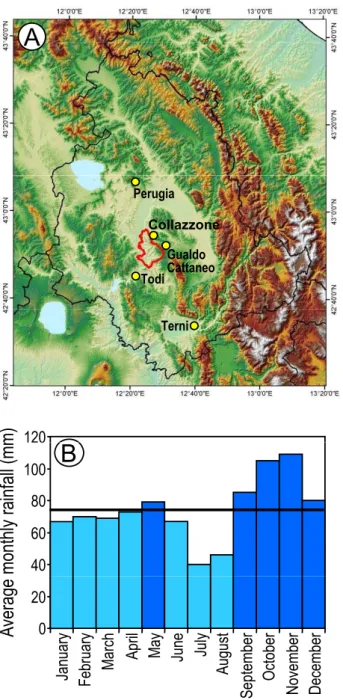
Fig. 1. (A) Map portraying terrain morphology in Umbria,

cen-tral Italy, and location of the Collazzone study area, shown by red line. (B) Average monthly rainfall for Collazzone area. Rainfall data for the Casalina rain gauge cover the 80-year period from 1921 to 2001. Thick black line shows monthly average. Light blue bars show months below average, and dark blue bars show months above average.

reports (e.g., newspaper articles, radio and television pro-grams, etc.). A combination of these techniques is often used.

Regardless of the adopted technique, preparing a landslide event inventory map is a difficult and time-consuming task. In this work, we report on an experiment aimed at exploiting

high resolution elevation data obtained by an Airborne Laser Scanner (ALS) to identify and map recent rainfall-induced landslides in Umbria, Central Italy.

2 Lidar technology

There are many methods that can be used to collect elevation data, including conventional ground surveys, digital pho-togrammetry, remote sensing, and Lidar (Ackermann, 1999; Kovalev and Eichinger, 2004; Lillesand et al., 2004). Lidar is an active sensory system that uses laser light to measure dis-tances. When mounted in an airborne platform, this device can rapidly measure distances between the sensor on the air-borne platform and points on the ground to collect and gen-erate densely spaced and highly accurate elevation data. The use of Lidar technology for accurate determination of terrain elevation began in the late 1970s (Ackermann, 1999; Lille-sand et al., 2004). Modern Lidar acquisition has typically an aircraft equipped with single or multiple airborne ground po-sitioning systems (GPS), an inertial measuring unit (IMU), a rapidly pulsing laser (from 20 000 to 50 000 pulses/s), and an adequate computer support. The Lidar system requires a sur-veyed ground base location to establish the accuracy of the Lidar data (Lillesand et al., 2004). Modern Lidar technology is well suited for the generation of high resolution Digital Elevation Models (DEM) (Ackermann, 1999; Kovalev and Eichinger, 2004; Lillesand et al., 2004).

3 Study area

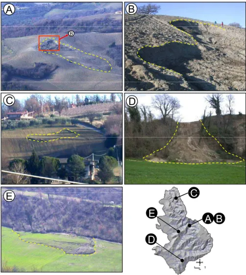
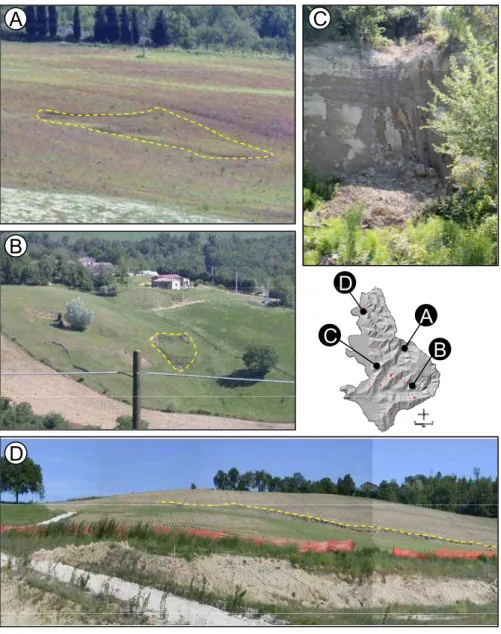
The study area extends for about 90 km2in central Umbria, Italy, in the municipalities of Collazzone, Todi and Gualdo Cattaneo (Fig. 1a). In the area, elevation ranges from 145 m along the Tiber River flood plain to 634 m at Monte di Grutti. Terrain gradient computed from a 10 m×10 m DEM ranges from 0◦ _{to 63.7}◦ _{degree, with a mean value of 9.9}◦ _{and a} standard deviation of 6.4◦_{. Landscape is hilly, and lithology} and the attitude of bedding planes control the morphology of the slopes. Sedimentary rocks crop out in the area, includ-ing (i) fluvial deposits, (ii) continental gravel, sand and clay, (iii) travertine, (iv) layered sandstone and marl in various percentages, and (v) thinly layered limestone (Conti et al., 1977; Servizio Geologico Nazionale, 1980; Cencetti, 1990; Barchi et al., 1991). Climate is Mediterranean, annual rain-fall averages 884 mm, and precipitation is most abundant in the period from September to December (Fig. 1b). Snow falls more or less every year, but reaches a depth greater than a few centimetres only about every five years. Rainfall and snowmelt-induced landslides are abundant in the area, and range in type and volume from large translational slides to deep and shallow flows (Guzzetti et al., 2006a; Galli et al., 2007) (Fig. 2).

A

B

C

D

E

C

E

D

B

A

E

C

Fig. 2. Typical landslides in the Collazzone area. Yellow dashed lines show landslide boundary. (A) Translational slide. Red box shows

location of (B). (B) Detail of the scarp area of the translational slide shown in (A). (C) Shallow soil slide. (D) Shallow disrupted slide. (E) Compound slide – earth flow.

4 Available data

For the study area, landslide and topographic information was available in digital format, including: (i) a multi-temporal landslide inventory map, at 1:10 000 scale, (ii) a reconnaissance landslide event inventory map showing land-slides triggered by rainfall in April 2004, (iii) a medium res-olution (10 m×10 m) Digital Elevation Model (DEM10), and

(iv) a high resolution (2 m×2 m) Digital Elevation Model (DEM2).

4.1 Multi-temporal landslide inventory

A multi-temporal landslide inventory map was available for the Collazzone study area. The map was prepared at 1:10 000 scale through the systematic interpretation of five sets of aerial photographs flown in the period from 1941 to 1997,

and geomorphological field mapping conducted from 1998 to 2003 following periods of prolonged rainfall (Guzzetti et al., 2006a; Galli et al., 2007).

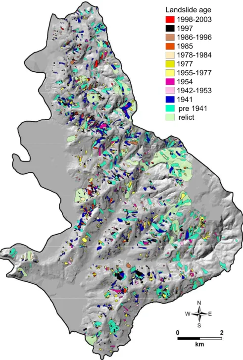
The multi-temporal inventory map shows 2564 landslides (Fig. 3), for a total landslide area of 22.1 km2, corresponding to a landslide density of 32.5 slope failures per square kilo-metre in the hilly portion of the study area. Due to geograph-ical overlap of landslides of different periods, the total area affected by landslides is 16.5 km2, 20.9% of the hilly portion of the study area. The total area affected by landslides is the area of slope surface disturbed by landslides, including the crown, transport, and depositional areas. Mapped landslides extend in size from 78 m2to 1.45×106m2(mean=8634 m2, median=2741 m2, std. dev.=36 181 m2). The most abundant failures shown in the map have an area of about 815 m2.

1998-2003 1997 1986-1996 Landslide age 1985 1978-1984 1977 1955-1977 1954 1942-1953 1942 1953 1941 pre 1941 relict

Fig. 3. Multi-temporal inventory map for the Collazzone area (Guzzetti et al., 2006a; Galli et al., 2007). Shaded relief image of the study

area obtained from a medium-resolution (10 m×10 m) Digital Elevation Model (DEM10).

4.2 Landslide event inventory

The period from December to April 2004 was wet in Umbria and rainfall-induced landslides occurred at several sites, in-cluding the Collazzone area. To map recent rainfall-induced landslides in the Collazzone area, four geomorphologists conducted a reconnaissance field survey driving and walk-ing systematically along main, secondary, and farm roads present in the study area. Geomorphologists stopped where

single or multiple landslides were identified, and at viewing points to check individual and multiple slopes. In the field, single and pseudo-stereoscopic photographs of each land-slide or group of landland-slides were taken. The photographs were used to locate the landslides on the topographic maps, to help characterize the type and the size of the mass move-ments, and to determine the local terrain gradient. Landslides identified in the field and in the photographs were mapped at 1:10 000 scale using topographic base maps (CTR) published

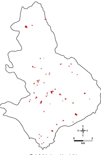
in 1999 (Fig. 4). The recent landslides were mostly shallow and with fewer deep-seated failures (Fig. 5). Shallow failures were classified as soil slides (62 failures) or compound slide – earth flows (3 failures). Deep-seated failures (5 failures) were translational slide or complex mass movements. Most of the recent rainfall-induced landslides occurred in culti-vated or barren areas. No landslide was identified in forested terrain.

The resulting reconnaissance landslide event inventory map (Fig. 4) shows 70 landslides ranging in size from 97 m2 to about 3.2×104m2(mean=3812 m2, median=1443 m2, std. dev.=5277 m2), for a total landslide area of 2.7×105m2, 0.34% of the hilly portion of the study area. The most abun-dant failures shown in the event inventory map have an area of about 1500 m2.

4.3 Medium resolution Digital Elevation Model

For the study area, a medium resolution DEM with a ground resolution of 10 m×10 m was available (DEM10)(Fig. 3).

The DEM10 was prepared by automatic interpolation of

10- and 5-m interval contour lines obtained from the same 1:10 000 scale topographic maps used to map the landslides. First, Intergraph® Terrain Analyst™ version 7.01 was used to build a Triangulated Irregular Network (TIN) of eleva-tion values from the contour lines. In the process, automatic break lines generation was used to infer relevant morpholog-ical features. Next, terrain elevation at grid nodes spaced 10 m×10 m on the ground was determined through weighted linear interpolation.

4.4 High resolution Digital Elevation Model

On 3 May 2004, a Dornier 228-110 aircraft operated by the Airborne Research and Survey Facility (ARSF) of the UK National Environment Research Council (NERC) flew an Optech Airborne Laser Terrain Mapper (ALTM) 3033 (Fig. 6) over the Collazzone area, and performed an Air-borne Lidar Swath Mapping (ALSM). The high-accuracy laser rangefinder collected an average of 33 000 laser obser-vations per second from an average flying height of about 2800 m, corresponding to an average distance to the ground of 2200 to 2650 m. First pulse, last pulse and intensity data were recorded. To guarantee the correct data localization, two GPS stations were installed in the study area with an ac-quisition time of one second. The Lidar data were processed by the Unit of Landscape Modelling of Cambridge Univer-sity. GPS post-processing was performed using Applanix PosPac version 3.02 software, and laser data post-processing was performed using Optech’s REALM version 3.03d soft-ware. No correction was performed to remove the effect of the forest cover, or side-lap effects between adjacent Lidar acquisition strips. The result was a cloud of 55.7 million elevation points covering an area of about 230 km2 encom-passing the Collazzone study area. In the study area, about

Rainfall-induced landslide

April 2004

Fig. 4. Landslide event inventory map showing rainfall-induced

landslides occurred in April 2004 in the the Collazzone area.

21.8 million elevation points were collected, for an average density of one point every 4.1 m2. ESRI® ArcGIS™ version 8.3 was used to transform the cloud of irregularly spaced el-evation points to a regular grid of elel-evation values spaced 2 m×2 m on the ground (DEM2)(Fig. 7).

5 Analysis and discussion

The landslide and topographic information was used to per-form three analyses in the Collazzone area. The first analysis consisted in establishing the extent to which the Lidar ele-vation data obtained by ALSM can be used to identify and map the recent rainfall-induced landslides. The second anal-ysis consisted in comparing statistics of landslide area ob-tained from the reconnaissance field inventory and a revised (corrected) inventory obtained exploiting the Lidar elevation information. The third analysis was aimed at comparing the

A

C

B

D

A

B

D

C

D

Fig. 5. Recent rainfall induced landslides mapped during a reconnaissance field survey conducted in April 2004 in the Collazzone area.

Yellow dashed lines show landslide boundary. (A) Shallow soil slide. (B) Shallow compound slide – earth flow. (C) Shallow disrupted slide.

(D) Crown area of deep-seated translational slide.

topographic signature (Pike, 1988) captured by the two avail-able DEMs in landslide and in stavail-able areas.

5.1 Identification and mapping of recent rainfall induced landslides

Recent rainfall-induced landslides in the Collazzone area left discernable morphological features on the topographic sur-face (Fig. 5). Recognition of these morphological features allowed geomorphologists to identify and map the new land-slides during the reconnaissance field survey. We tested the possibility of using the high resolution DEM2 acquired by

ALSM shortly after landslide occurrence, to identify, locate and map the recent slope failures. Since the effects of forest

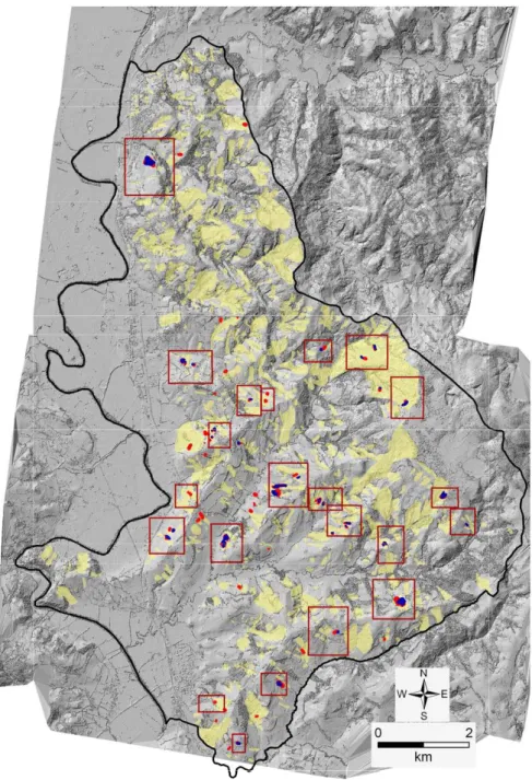
and ALSM side-laps were not removed from the Lidar eleva-tion data, the test was performed in a reduced poreleva-tion of the study area free of forest and not affected by side-lap effects. The reduced portion corresponds to 22 sub-areas (red boxes in Fig. 7) collectively covering 10.9 km2(12.2% of the study area and 13.8% of the hilly portion of the study area), and en-compassing representative topography and landslide types.

Derivate maps showing topography in the selected sub-areas were obtained from the high-resolution DEM2. For

each sub-area, a shaded relief image, a slope map, and a contour map (one-meter interval) were prepared. The three derivative maps were inspected visually – singularly and in combination – for morphological features indicative of

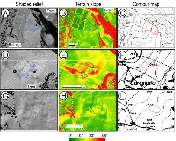
re-cent landslides. The result was a revised landslide event in-ventory map for the 22 selected sub-areas (Fig. 7). Figure 8 shows three examples of landslides mapped through visual inspection of the derivative maps obtained from DEM2.

Results of the test showed that Lidar elevation data are use-ful for the identification and mapping of the recent rainfall-induced landslides in the Collazzone area. More precisely:

(i) Deep-seated landslides exhibited morphological fea-tures visible in the shaded relief images and the slope maps (Fig. 8a–c). Field inspection of the deep-seated landslides revealed that the escarpments bounding the crown areas ranged from about 0.5 m to more than 3 m, and that surface displacements caused by the landslides (e.g., fractured blocks, hummocks, pressure ridges, de-pressions, etc.) ranged in local relief from a few decime-tres to more than 2 m. In the shaded relief images, scarps and ground fractures in the landslide crown area, hummocky topography in the landslide deposit, and lo-bate forms at the landslide toe, were apparent (Fig. 8). The boundaries of the landslide deposit and of the crown area were also visible in the slope maps (Fig. 8). (ii) Compound, mostly shallow slide – earth flows were

characterized by morphological features less distinct than those typical of deep-seated landslides (Fig. 8d– f). In places, these morphological features (e.g., escarp-ments, cracks, hummocks, pressure ridges, etc.) were discernible in the shaded relief images and in the slope map, allowing for the identification and mapping of the rainfall-induced landslides. In other places, the mor-phological features of shallow slide – earth flows were not clearly visible in the derivative topographic maps. These features could not be attributed univocally to a landslide, making the identification and mapping of the rainfall-induced slope failures uncertain or impossible. (iii) Shallow soil slides were small, and left faint

morpho-logical signs on the topographic surface (Fig. 8g–i). Field inspection of some of the mapped soil slides re-vealed that surface deformation in the crown area was less than 0.5 m, and in places less than 0.2 m. These fea-tures were generally not distinguishable in the shaded relief images and the slope maps (Fig. 8), and soil slides could not be mapped from the digital derivative topo-graphic maps.

It should be noted that the same team of geomorpholo-gists that performed the reconnaissance field mapping per-formed the visual analysis of the digital terrain derivative maps. When performing the visual analysis of the derivative maps, the interpreters were informed of the type, abundance, and approximate location of the rainfall-induced landslides. This has introduced a bias in the identification of the land-slides. It remains undetermined the extent to which the re-cent rainfall-induced landslides in the Collazzone area – and

A

B

Fig. 6. (A) Dornier 228-110 aircraft operated by the Airborne

search and Survey Facility of the UK National Environment Re-search Council that flew the Optech’s Airborne Laser Terrain Map-per 3033, shown by the arrow in (B).

elsewhere in Umbria – could be identified and mapped accu-rately solely from the visual interpretation of the digital ter-rain maps, i.e., without previous information on the location and type of the slope failures.

5.2 Comparison of the inventories

The original landslide-event reconnaissance mapping and the revised landslide event mapping updated exploiting the Lidar elevation data were compared in the 22 sub-areas where both inventories are available (Fig. 7). Comparison was aimed at verifying differences in the number, size, and position of the mapped landslides.

In the 22 selected sub-areas, the original reconnaissance field inventory map shows 37 landslides, ranging in size from 165 m2to 31 910 m2, for a total landslide area of 193 046 m2 (Table 1). In the same 22 sub-areas, the revised inventory map shows 47 landslides, ranging in size from 60 m2 to

Fig. 7. Shaded relief image encompassing the Collazzone study area (shown by dark black line) prepared from a 2 m×2 m Digital Elevation

Model (DEM₂)obtained interpolating 55.7 million elevation data collected by an Airborne Laser Scanner on 3 May 2004. Light yellow polygons are pre-existing landslides shown in the multi-temporal inventory (Fig. 3). Red polygons show recent rainfall-induced landslides mapped through reconnaissance field survey in April 2004 (Fig. 4). Blue polygons show revised inventory prepared exploiting derivative topographic maps obtained from DEM2. Red boxes indicate 22 sub-areas selected for a comparison of the inventories.

25 900 m2, for a total landslide area of 118 439 m2. The re-vised inventory map shows 27% more landslides and 39% less total landslide area. This corresponds to a smaller average (2520 m2 vs. 5219 m2) and median (1128 m2 vs. 2812 m2)landslide sizes (Table 1).

Statistics of landslide areas for the two inventory maps are summarised in Fig. 9, for all the mapped landslides, and for

the deep-seated and the shallow landslides. Inspection of the box plots reveals that the revised inventory map shows smaller landslides, for all landslide types. The area of the individual landslides mapped during the original reconnais-sance field survey was larger than the area of the same land-slides mapped using the Lidar elevation data. Reasons for the differences are manifold, including: (i) perspective,

lo-Shaded relief

Terrain slope

Contour map

A

B

C

D

E

F

G

H

I

Fig. 8. Examples of recent rainfall-induced landslides mapped in the Collazzone area. Red lines show landslides identified and mapped

during the reconnaissance field surveys. Blue lines show landslides identified and mapped using derivative topographic maps obtained from

DEM2. Shaded relief images show 1-m contour lines obtained from DEM2. Contour maps portray 10- and 5-m contour lines and other

topographic features shown in the CTR base maps. (A), (B), (C) deep-seated translational slide. (D), (E), (F) compound slide – earth flows.

(G), (H), (I) shallow soil slide.

cally incomplete or inaccurate, view of the landslide in the field, (ii) poor or incorrect representation of the topographic surface in the base map used to map landslides in the field, and (iii) limited time available to the geomorphologists to map the individual landslides in the field.

Visual comparison of the two inventories in the 22 selected sub-areas indicates that the revised inventory map shows landslide boundaries with an improved cartographic detail. In the adjusted inventory map, individual landslides match more accurately the representation of topography provided by the one meter contour lines, than the same landslides shown in the field inventory and mapped on the CTR to-pographic base maps. The CTR maps show a topography that predates the new landslides, making it difficult for the geomorphologists to map the landslides accurately, particu-larly small landslides in cultivated fields or grassland areas. The Lidar elevation data were acquired shortly after the oc-currence of the rainfall-induced landslides, and captured the changed (altered) morphology. This facilitated the accurate mapping of the recent landslides.

Table 1. Collazzone study area, central Umbria. Characteristics of

landslide event inventory maps for 22 selected sub-areas. (A) Orig-inal reconnaissance inventory map obtained through field surveys. (B) Revised inventory map prepared exploiting derivative maps ob-tained from DEM2.

A B

Number of mapped landslides # 37 47

Total landslide area m2 193 046 118 439

Minimum landslide area m2 165 60

Maximum landslide area m2 31 910 25 900

Mean landslide area m2 5219 2520

Median landslide area m2 2812 1128

Standard deviation of landslide area m2 6835 4450

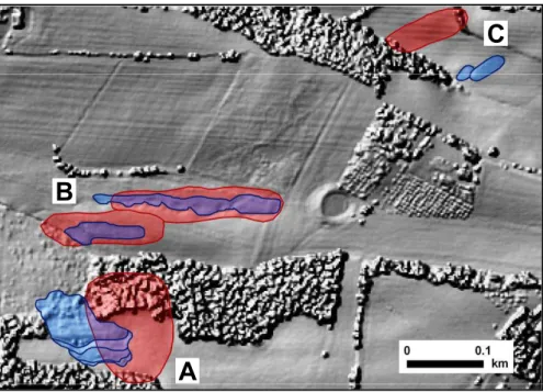
Figure 10 summarizes typical mismatches between land-slides shown in the original reconnaissance inventory (shown in red) and landslides portrayed in the revised inventory

35,000 Shallow landslides Deep-seated landslides All landslides Outlier de A re a (m 2) 15,000 20,000 25,000 30,000 50th 25th 75th Mean 10th Outlier 90th La nd sl id 0 5,000 10,000

(A) Reconnaissance landslide mapping

(B) Revised landslide mapping

A B A B A B

Fig. 9. Comparison of the statistics of landslide area obtained from

the original reconnaissance inventory map (red) and the inventory revised using derivative maps obtained from the Lidar elevation data (blue) in 22 selected sub-areas (see Fig. 7). Box plots are shown for all landslides, for deep-seated landslides, and for shallow land-slides.

(shown in blue). Some of the landslides were mapped in a slightly different geographical location (Fig. 10a). Other landslides were mapped in the same geographical location but the extent of the landslide was larger (overestimated) in the reconnaissance inventory (Fig. 10b). In places, a single (larger) landslide was mapped in the reconnaissance inven-tory, where the same morphological features were attributed to multiple (smaller) landslides in the revised inventory map (Fig. 10c).

To quantify the geographical mismatch between the two inventory maps, the method proposed by Carrara et al. (1992) was adopted. For the purpose, the overall mapping error in-dex, E, was computed

E = (A ∪ B) − (A ∩ B)

(A ∪ B) , 0 ≤ E ≤ 1 (1)

where A and B are the total landslide area in the first (origi-nal) and in the second (revised) inventory map, respectively, and ∪ and ∩ are the geographical union and intersection of the two inventory maps. From Eq. (1), the degree of match-ing, M, between two inventory maps (Galli et al., 2007) is

M =1 − E, 0 ≤ M ≤ 1 (2)

If two inventory maps show exactly the same landslides in the same positions (a rather improbable situation) matching is perfect (M=1) and mapping error is null (E=0). If two

landslide maps are completely different, cartographic match-ing is null (M=0) and mappmatch-ing error is maximum (E=1) (Galli et al., 2007).

Geographical union (∪) and intersection (∩) of the orig-inal and the revised inventory maps was performed in a GIS. The obtained figures were used to compute the map-ping error index (E) and the cartographic matching index (M). Geographical union of the two inventory maps was 2.36×105m2, and landslide area common to both inventory maps was 7.50×104m2(Fig. 10). From Eq. (1) and Eq. (2), the map error index E was 0.68 and the map match index

M was 0.32. These figures indicate a significant discrep-ancy between the two inventories (Galli et al., 2007). We attribute the large geographical mismatch to mapping errors in the original field inventory. Inspection of the largest dis-crepancies revealed that most of the errors were due primar-ily to: (i) the locally poor quality of the base maps used to map the landslides in the field, and (ii) the lack of a complete (vertical) view of the landslides in the field.

5.3 Comparison of Digital Elevation Models

The last test consisted in evaluating how well DEM2 and

DEM10 captured the topographic signature of landslide

ter-rain (Pike, 1988). For the purpose, three slopes with differ-ent landslide abundance and failures of differdiffer-ent ages were selected, including (Fig. 11): (i) a slope free of known landslides, (ii) a slope where recent (April 2004) and pre-existing (1941–1997) landslides were identified, and (iii) a slope where only pre-existing (1941–1997) landslides were known.

Maps of the local terrain gradient were prepared for the three selected slopes, and their descriptive statistics com-pared. Results, summarized in Fig. 12, reveal that the higher resolution DEM2 captured a more diversified topography

than the coarser resolution DEM10. The consistently larger

range of terrain gradient shown by DEM2 reveals this,

al-though the average and the median values of terrain gradient are about the same for the two DEMs (Fig. 12). DEM2shows

steeper or much steeper terrain and a considerably larger pro-portion of steep terrain, for all the considered slopes.

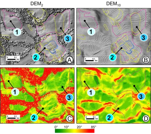
Joint inspection of Figs. 11 and 12 allows for additional considerations on how well the two DEMs captured – or did not capture – the topographic signature of landslides. Differences in the statistics of terrain gradient are largest where recent (April 2004) and pre-existing (1941–1997) landslides were recognized (slope #2 in Fig. 11), are signif-icant where only pre-existing (1941–1997) landslides were mapped (slope #3 in Fig. 11), and are smallest in the slope free of known landslides (slope #1 in Fig. 11). The differ-ences suggest that the two DEMs captured landslide mor-phology differently.

Immediately after a landslide event, individual landslides are “fresh” and usually clearly recognizable (Malamud et al., 2004). Landslide morphology becomes increasingly

indis-C

B

A

Fig. 10. Typical differences between landslides shown in the original reconnaissance inventory map (shown in red), and landslides shown in

the revised inventory map prepared exploiting derivative topographic maps obtained from DEM2(shown in blue).

tinct with the age of the landslide (McCalpin, 1984). This is caused by various factors, including local adjustments of a landslide to the new morphological setting, new landslides, erosion, land use changes, and human actions (e.g., plough-ing). In the Collazzone area, distinct morphological features (e.g., scarps, ridges, hummocks, cracks, sinks, etc.) char-acterize the recent rainfall-induced landslides. These fea-tures contribute to “fresh” landslide morphology, well cap-tured by DEM2 but inadequately shown by the lower

res-olution DEM10 (slope #2 in Fig. 11). In the study area,

old (pre-existing and 1941–1997) landslides exhibit a typi-cal “smoothed” morphology, characterized by curved hum-mocks, poorly distinct rounded escarpments, and gentle slopes. This morphology is well captured by DEM2 and is

partially captured by DEM10 (slope #3 in Fig. 11). Where

no landslides have occurred (slope #1 in Fig. 11), slopes are regular and their morphology controlled by lithology and the attitude of bedding planes. The morphology of stable slopes is (almost) equally well captured by DEM2 and DEM10.

We conclude that the improved topographic information pro-vided by DEM2is significant where recent rainfall-induced

landslides have occurred, and is much less significant in im-proving the representation of stable (landslide free) slopes.

6 Conclusions

Landslide inventory maps are important sources of informa-tion for landslide susceptibility, hazard and risk assessment (Guzzetti et al., 2000; Galli et al., 2007). Landslide event

inventory maps are particularly significant because – if prop-erly prepared – they are nearly complete, i.e., they show all the landslides produced by an individual landslide trigger (e.g., a rainstorm, an earthquake, a rapid snowmelt event). Preparing a complete landslide event inventory map is diffi-cult, and geomorphologists have experimented with methods to reduce the time and costs for the production of landslide event inventories. In this work, we have reported on an ex-periment aimed at exploiting high-resolution elevation data obtained by an airborne laser scanner (ALS) to map recent rainfall-induced landslides in Umbria, central Italy.

For the Collazzone area, digital elevation data were ob-tained by Airborne Lidar Swath Mapping on 3 May 2004, shortly after a prolonged period of rainfall that resulted in numerous landslides in the study area. Field surveys con-ducted immediately after the rainfall period allowed mapping 70 landslides in the Collazzone area, for a total landslide area of 2.7×105m2. Successively, the Lidar elevation data were interpolated to obtain a 2 m×2 m Digital Elevation Model (DEM2). The high-resolution DEM2 was used to assess

whether the Lidar elevation data could be exploited to map the recent rainfall-induced landslides. Shaded relief images and slope maps obtained from DEM2 for 22 selected

sub-areas were used to update the reconnaissance landslide inven-tory. Inspection of the revised inventory revealed that land-slides mapped exploiting the Lidar elevation data matched to-pography more accurately than the same landslides mapped using the pre-existing topographic maps. In the 22 selected sub-areas, the revised inventory showed 27% more landslides

DEM

DEM

2

1

3

2

1

3

2

2

A

B

2

1

3

2

1

3

C

D

Fig. 11. Comparison of two DEMs in stable and in landslide areas. (A) Shaded relief obtained from DEM2. (B) Shaded relief derived from DEM₁₀, 1-m contour lines are shown. (C) Map of terrain gradient (slope) obtained from DEM₂. (D) Map of terrain gradient (slope) obtained from DEM10. Yellow lines show pre-existing landslides, and blue lines show recent (April 2004) rainfall-induced landslides. Purple lines show selected slopes. Coloured numbers indicate: (1) a slope free of known landslides, (2) a slope with recent (April 2004) and pre-existing (1941–1997) known landslides, and (3) a slope with only pre-existing (1941–1997) known landslides.

35 2 1 3 _90thOutlier 20 25 30 a d ie n t (° ) 50th 25th 75th Mean 10th Outlier 90th 5 10 15 T e rra in g ra 0

DEM₂ DEM₁₀ DEM₂ DEM₁₀ DEM₂ DEM₁₀

Fig. 12. Comparison of terrain gradient statistics obtained from

DEM2and DEM10in three selected slopes (see Fig. 11). (1) Slope free of known landslides, (2) slope with recent (April 2004) and existing (1941–1997) known landslides, (3) slope with only pre-existing (1941–1997) known landslides.

and 39% less landslide area, corresponding to a smaller av-erage landslide size. This is important information for ge-omorphologists interested in the statistics of landslide areas (e.g., Malamud et al., 2004), and has implications for the assessment of landslide hazard (Guzzetti et al., 2006a) and for the validation of landslide hazard forecasts (Guzzetti et al., 2006b). Since the geomorphologists that performed the visual analysis of the derivative topographic maps were in-formed of the presence of the rainfall-induced landslides, it remains undetermined the extent to which the recent land-slides in the Collazzone area could be mapped accurately solely from the visual interpretation of the digital terrain maps.

Further analysis of the discrepancy between the original reconnaissance inventory map and the revised inventory re-vealed locally significant differences that were attributed to mapping errors and imprecision mostly in the reconnaissance field inventory. The errors and the imprecision were at-tributed chiefly to: (i) the incomplete or inaccurate view of some the landslides in the field, (ii) the locally imprecise rep-resentation of the topographic surface in the base maps used to map the landslides, and (iii) the limited time available to map the new landslides in the field.

Finally, the high resolution DEM2 was compared to the

pre-existing, coarser resolution (10 m×10 m), DEM10to

es-tablish how well the two digital representations of topogra-phy captured the topographic signature of landslides. Re-sults indicate that the higher resolution DEM2was capable

of capturing a more diversified topography than the coarser resolution DEM10. Differences in the statistics of terrain

gra-dient obtained from the two DEMs were largest where recent and pre-existing landslides were present, intermediate where only pre-existing landslides were present, and reduced in ar-eas free of known landslides. The finding has implications for the recognition and mapping of landslides, and may lead to the automatic or semi-automatic extraction of landslide features from high resolution DEMs obtained from Lidar el-evation data.

Acknowledgements. We are grateful to M. Jaboyedoff and to a second anonymous referee for their constructive comments. We express gratitude to N. Hovius for making the Lidar survey possible, and C. P. Stark for field assistance. The Airborne Remote Sensing Facility of the U.K. National Environmental Research Council flew the Laser Terrain Mapper. The Unit of Landscape Modelling of Cambridge University processed the Lidar data. Work partly financed by CNR – IRPI, CNR – GNDCI, and ASI MORFEO grants.

Edited by: T. Glade

Reviewed by: M. Jaboyedoff and another anonymous referee

References

Ackermann, F.: Airborne Laser Scanning – Present status and fu-ture expectations, ISPR Journal of Photogrammetry & Remote Sensing, 54, 64–67, 1999.

Barchi, M., Brozzetti, F., and Lavecchia, G.: Analisi strutturale e geometrica dei bacini della media valle del Tevere e della valle umbra. Bollettino Societ`a Geologica Italiana, 110, 65–76 (in Ital-ian), 1991.

Brunsden, D.: Landslide types, mechanisms, recognition, identifi-cation, in: Landslides in the South Wales coalfield, edited by: Morgan, C. S., Proceedings Symposium, April 1–3, The Poly-technic of Wales, 19–28, 1985.

Brunsden, D.: Mass movements; the research frontier and beyond: a geomorphological approach, Geomorphology, 7, 85–128, 1993. Bucknam, R. C., Coe, J. A., Chavarria, M. M., Godt, J. W., Tarr,

A. C., Bradley, L.-A., Rafferty, S., Hancock, D., Dart, R. L., and Johnson, M. L.: Landslides Triggered by Hurricane Mitch in Guatemala – Inventory and Discussion, U.S. Geological Survey Open File Report 01-443, 2001.

Cardinali, M., Ardizzone, F., Galli, M., Guzzetti, F., and Reichen-bach, P.: Landslides triggered by rapid snow melting: the De-cember 1996–January 1997 event in Central Italy, in: Proceed-ings 1st EGS Plinius Conference, edited by: Claps, P. and Sic-cardi, F., Maratea, Bios Publisher, Cosenza, 439–448, 2001. Cardinali, M., Galli, M., Guzzetti, F., Ardizzone, F., Reichenbach,

P., and Bartoccini, P.: Rainfall induced landslides in December 2004 in South-Western Umbria, Central Italy, Nat. Hazards Earth

Syst. Sci., 6, 237–260, 2006,

http://www.nat-hazards-earth-syst-sci.net/6/237/2006/.

Carrara, M. Cardinali, M., and Guzzetti, F.: Uncertainty in assess-ing landslide hazard and risk, ITC Journal, 2, 172–183, 1992. Catani, F., Farina, P., Moretti, S., Nico, G., and Strozzi, T. On the

application of SAR interferometry to geomorphological studies: estimation of landform attributes and mass movements, Geomor-phology, 66, 1–4, 119–131, 2005.

Cencetti, C. Il Villafranchiano della “riva umbra” del F. Tevere: ele-menti di geomorfologia e di neotettonica, Bollettino Societ`a Ge-ologica Italiana, 109, 2, 337–350 (in Italian), 1990.

CENR/IWGEO: Strategic Plan for the U.S. Integrated Earth Ob-servation System. National Science and Technology Council Committee on Environment and Natural Resources, Washington, D.C., available at http://iwgeo.ssc.nasa.gov, 2005.

Cheng, K. S., Wei, C., and Chang, S. C.: Locating landslides using multi-temporal satellite images, Adv. Space Res., 33, 3, 96–301, 2004.

Conti, M. A. and Girotti, O.: Il Villafranchiano nel “Lago Tiberino”, ramo sud-occidentale: schema stratigrafico e tettonico, Geologia Romana, 16, 67–80 (in Italian), 1977.

Czuchlewski, K. R., Weissel, J. K., and Kim, Y.: Polarimetric syn-thetic aperture radar study of the Tsaoling landslide generated by the 1999 Chi-Chi earthquake, Taiwan, J. Geophys. Res., 108(F1), 7/1–10, 6006, doi:10.1029/2003JF000037, 2003.

Franklin, A. J.: Slope instrumentation and monitoring, in: Slope Instability, edited by: Brunsden, D. and Prior, D. B., John Wiley and Sons, 1–25, 1984.

Galli, M., Ardizzone, F., Cardinali, M., Guzzetti, F., and Reichen-bach, P.: Comparison of landslide inventory maps, Geomorphol-ogy, in press, 2007.

Guzzetti, F., Cardinali, M., Reichenbach, P., and Carrara, A.: Com-paring landslide maps: A case study in the upper Tiber River Basin, central Italy, Environ. Manage., 25, 3, 247–363, 2000. Guzzetti, F., Cardinali, M., Reichenbach, P., Cipolla, F., Sebastiani,

C., Galli, M., and Salvati, P.: Landslides triggered by the 23 November 2000 rainfall event in the Imperia Province, Western Liguria, Italy, Eng. Geol., 73, 2, 229–245, 2004.

Guzzetti, F., Galli, M., Reichenbach, P., Ardizzone F., and Cardi-nali, M.: Landslide hazard assessment in the Collazzone area, Umbria, central Italy, Nat. Hazards Earth Syst. Sci., 6, 115–131, 2006a.

Guzzetti, F., Malamud, B. D., Turcotte, D. L., and Reichenbach, P.: Power-law correlations of landslide areas in Central Italy, Earth Planet. Sci. Lett., 195, 169–183, 2002.

Guzzetti, F., Reichenbach, P., Ardizzone, F., Cardinali, M., and Galli, M.: Estimating the quality of landslide susceptibility mod-els, Geomorphology, 81, 166–184, 2006b.

Hansen, A.: Landslide hazard analysis, in: Slope instability, edited by: Brunsden, D. and Prior, D. B., Wiley & Sons, New York, 523–602, 1984.

Harp, E. L. and Jibson, R. L.: Landslides triggered by the 1994 Northridge, California earthquake, Seismological Society of America Bulletin, 86, S319–S332, 1996.

Hilley, G. E., B¨urgmann, R., Ferretti, A., Novali, F., and Rocca, F.: Dynamics of Slow-Moving Landslides from Permanent Scatterer Analysis, Science, 304, 1952–1955, 2004.

IGOS Geohazards: IGOS Geohazards Theme Report, April 2003, European Space Agency, Data User Programme, http://dup.esrin.

esa.it/igos-geohazards, 2003.

K¨a¨ab, A.: Monitoring high-mountain terrain deformation from re-peated air- and spaceborne optical data: examples using digital aerial imagery and ASTER data ISPRS, Journal of Photogram-metry and Remote Sensing, 57, 1–2, 39–52, 2002.

Kovalev, V. A. and Eichinger, W. E.: Elastic Lidar: Theory, Prac-tice, and Analysis Methods, Resources for John Wiley & Sons INC., 615 pp., 2004.

Lillesand, T. M., Kiefer, R. W., and Chipman J. W.: Remote sens-ing and image interpretation, J. Wiley & Sons, United States of America, 5th edition, 763 pp., 2004.

Malamud, B. D., Turcotte, D. L., Guzzetti, F., and Reichenbach, P.: Landslide inventories and their statistical properties, Earth Surf. Proc. Land., 29, 6, 687–711, 2004.

Mantovani, F., Soeters, R., and van Westen, C. J.: Remote sensing techniques for landslide studies and hazard zonation in Europe, Geomorphology, 15, 213–225, 1996.

McCalpin, J.: Preliminary age classification of landslides for inven-tory mapping, Proceedings 21st annual Engineering Geology and Soils Engineering Symposium, Moscow, Idaho, 99–111, 1984. McKean, J. and Roering, J.: Objective landslide detection and

sur-face morphology mapping using high-resolution airborne laser altimetry, Geomorphology, 57, 3–4, 331–351, 2003.

Paˇsek, J.: Landslide inventory, International Association Engineer-ing Geologist Bulletin, 12, 73–74, 1975.

Petley, D. J.: Ground investigation, sampling and testing for studies of slope instability, in: Slope instability, edited by: Brunsden, D. and Prior, D. B., Wiley, Chichester, 67–101, 1984.

Pike, R. J.: The geometric signature: quantifying landslide-terrain types from digital elevation models, Math. Geol., 20, 5, 491–511, 1988.

Reichenbach, P., Guzzetti, F., and Cardinali, M.: Map of sites his-torically affected by landslides and floods in Italy, 2nd edition, CNR Gruppo Nazionale per la Difesa dalle Catastrofi Idrogeo-logiche Publication n. 1786, scale 1:1 200 000, 1998.

Rib, H. T. and Liang, T.: Recognition and identification, in: Land-slide Analysis and Control, edited by: Schuster, R. L. and Krizek, R. J., National Academy of Sciences, Transportation Research Board Special Report 176, Washington, 34–80, 1978.

Salvati, P., Bianchi, C., and Guzzetti, F.: Catalogo delle Frane e delle Inondazioni Storiche in Umbria, CNR IRPI e Fondazione Cassa di Risparmio di Perugia, ISBN-10 88-95172-00-0, 278 pp., 2006.

Salvati, P., Guzzetti, F., Reichenbach, P., Cardinali, M., and Stark, C. P.: Map of landslides and floods with human consequences in Italy, CNR Gruppo Nazionale per la Difesa dalle Catastrofi Idrogeologiche Publication n. 2822, scale 1:1 200 000, 2003. Schulz, W. H.: Landslides mapped using LIDAR imagery, Seattle,

Washington, United States Geological Survey Open File Report 2004-1396, 2004.

Schulz, W. H.: Landslides Susceptibility Estimated From Mapping Using Light Detection and Ranging (LIDAR) Imagery and His-torical Landslide Records, Seattle, Washington, United States Geological Survey Open File Report 2005-1405, 2005.

Servizio Geologico Nazionale: Carta Geologica dell’Umbria, Map at 1:250 000 scale (legend in Italian), 1980.

Singhroy, V.: Remote sensing of landslides, in: Landslide risk as-sessment, edited by: Glade, T., Anderson, M. G., and Crozier, M. J., John Wiley, 469–492, 2005.

Singhroy, V. and Molch, K.: Characterizing and monitoring rock-slides from SAR techniques, Adv. Space Res., 33, 3, 290–295, 2004.

Turner, A. K. and Schuster, R. L. (Eds.): Landslides: Investiga-tion and MitigaInvestiga-tion, Washington, D.C., NaInvestiga-tional Research Coun-cil, Transportation Research Board Special Report 247, 673 pp., 1996.

Wieczorek, G. F.: Preparing a detailed landslide-inventory map for hazard evaluation and reduction, Bulletin Association Engineer-ing Geologists, 21, 3, 337–342, 1984.

Zinck, J. A., L´opez, J., Metternicht, G. I., Shrestha, D. P., and V´azquez-Selem, L.: Mapping and modelling mass movements and gullies in mountainous areas using remote sensing and GIS techniques, Int. J. Appl. Earth Obs., 3, 1, 43–53, 2001.