Meteorological implementation issues in chemistry and transport models

HAL Id: hal-00295980

https://hal.archives-ouvertes.fr/hal-00295980

Submitted on 12 Jul 2006

HAL is a multi-disciplinary open access

archive for the deposit and dissemination of

sci-entific research documents, whether they are

pub-lished or not. The documents may come from

teaching and research institutions in France or

abroad, or from public or private research centers.

L’archive ouverte pluridisciplinaire HAL, est

destinée au dépôt et à la diffusion de documents

scientifiques de niveau recherche, publiés ou non,

émanant des établissements d’enseignement et de

recherche français ou étrangers, des laboratoires

publics ou privés.

transport models

S. E. Strahan, B. C. Polansky

To cite this version:

S. E. Strahan, B. C. Polansky. Meteorological implementation issues in chemistry and transport

models. Atmospheric Chemistry and Physics, European Geosciences Union, 2006, 6 (10),

pp.2895-2910. �hal-00295980�

www.atmos-chem-phys.net/6/2895/2006/ © Author(s) 2006. This work is licensed under a Creative Commons License.

Chemistry

and Physics

Meteorological implementation issues in chemistry and transport

models

S. E. Strahan1and B. C. Polansky2

1_{University of Maryland Baltimore County, Goddard Earth Science and Technology Center, 5523 Research Park Dr., Suite}

320, Baltimore, MD, 21228, USA

2_{Science Systems and Applications, Inc., 10210 Greenbelt Rd., Suite 600, Lanham, MD, 20706, USA}

Received: 2 September 2005 – Published in Atmos. Chem. Phys. Discuss.: 21 October 2005 Revised: 13 January 2006 – Accepted: 14 April 2006 – Published: 12 July 2006

Abstract. Offline chemistry and transport models (CTMs)

are versatile tools for studying composition and climate is-sues requiring multi-decadal simulations. They are computa-tionally fast compared to coupled chemistry climate models, making them well-suited for integrating sensitivity experi-ments necessary for understanding model performance and interpreting results. The archived meteorological fields used by CTMs can be implemented with lower horizontal or verti-cal resolution than the original meteorologiverti-cal fields in order to shorten integration time, but the effects of these shortcuts on transport processes must be understood if the CTM is to have credibility. In this paper we present a series of sensitiv-ity experiments on a CTM using the Lin and Rood advection scheme, each differing from another by a single feature of the wind field implementation. Transport effects arising from changes in resolution and model lid height are evaluated us-ing process-oriented diagnostics that intercompare CH4, O3,

and age tracer carried in the simulations. Some of the diag-nostics used are derived from observations and are shown as a reality check for the model. Processes evaluated include tropical ascent, tropical-midlatitude exchange, poleward cir-culation in the upper stratosphere, and the development of the Antarctic vortex. We find that faithful representation of stratospheric transport in this CTM is possible with a full mesosphere, ∼1 km resolution in the lower stratosphere, and relatively low vertical resolution (>4 km spacing) in the mid-dle stratosphere and above, but lowering the lid from the up-per to lower mesosphere leads to less realistic constituent dis-tributions in the upper stratosphere. Ultimately, this affects the polar lower stratosphere, but the effects are greater for the Antarctic than the Arctic. The fidelity of lower stratospheric transport requires realistic tropical and high latitude mixing barriers which are produced at 2◦_×2.5◦_{, but not lower} reso-lution. At 2◦_×2.5◦ _{resolution, the CTM produces a vortex} capable of isolating perturbed chemistry (e.g. high Cly and low NOy)required for simulating polar ozone loss.

Correspondence to: S. E. Strahan

(sstrahan@pop600.gsfc.nasa.gov)

1 Introduction

In recent years, coupled chemistry climate models (CCMs) have been used to study complex atmospheric phenomena such as the recovery of the Antarctic ozone hole (Austin and Butchart, 2003; Tian and Chipperfield, 2005). The mod-els’ chemistry, dynamics, and radiation are fully coupled al-lowing the radiative properties of the constituents to feed-back into the radiation calculation, the radiation to affect the dynamics, the updated dynamics to then transport the con-stituents, and so on. Model experiments attempting to produce past observations or predict future climate states re-quire multi-decadal simulations, which, for a coupled climate model at reasonably high resolution, is computationally ex-pensive. The time and cost to perform additional sensitivity experiments with a coupled model, necessary for understand-ing its behavior, may be prohibitive.

An offline chemistry transport model (CTM) is a fre-quently used tool that simplifies model calculations by using archived meteorological fields, making multi-decadal sim-ulations tractable. Meteorological fields, generated from a general circulation model (GCM) or data assimilation system (DAS), are input into the CTM and updated several times per model day. The CTM lacks the ability to simulate feedbacks between the constituents, radiation, and dynamics, which may be large for ozone loss in the polar vortex (MacKen-zie and Harwood, 2000). This is, however, not necessarily a disadvantage for the CTM, as radiative coupling with ozone in the CCM will not lead to a more realistic simulation of ozone loss if the model has a cold pole problem (Austin, 2002). Constituent transport in a GCM will also be sensi-tive to resolution, but that sensitivity cannot readily be tested because physical parameterizations in the GCM are tuned to a particular resolution. A CTM has the advantage of being integrated much more quickly than a coupled model, which also allows - even encourages - its users to conduct sensitivity studies that increase the understanding of the model perfor-mance (e.g., sensitivity to boundary conditions, input wind fields, resolution, etc. ).

Previous studies have examined the differences in strato-spheric tracer transport between online and offline calcu-lations. Rasch et al. (1994) used daily averaged winds from the Middle Atmosphere Community Climate Model 2 (MACCM2) to transport simple tracers in an offline model and reported a significant speed up over the online calcula-tion. They found that many aspects of tracer transport were well represented, but mixing in the tropical lower strato-sphere was much slower than in the online calculation. This was attributed to using daily-averaged winds that eliminated the large transients in vertical velocities that may be respon-sible for significant vertical transport on short time scales. Waugh et al. (1997) experimented with temporal sampling of meteorological fields used in offline simulations and con-cluded that to obtain good agreement with the online cal-culation, multi-year CTM simulations would require winds sampled at least every 6 h.

CTMs are widely used for assessments because their rapid integration time makes it possible to run many sce-narios (e.g., IPCC, 2001). Their computational expediency is important for predicting atmospheric response on decadal timescales for problems such as ozone recovery and the ef-fects of increasing greenhouse gases on climate. In order to understand the long-term simulated behavior, a number of model sensitivity studies should be performed. For exam-ple, to understand a model’s response to the Mt. Pinatubo eruption requires simulations with and without volcanic ef-fects, and with different levels of chlorine-loading (Stolarski et al., 2006). If the CTM uses input meteorological fields with degraded resolution in order to decrease the integration time – for example, putting the 2◦_×2.5◦_{fields on a 4}◦_×5◦ grid, or reducing the number of vertical levels – how will this affect the representation of stratospheric processes? The assessment of CTM performance and sensitivity to inputs is vital to the credibility of CTM results and has been the hall-mark of the NASA Global Modeling Initiative (GMI), a CTM project that emphasizes process-oriented model evaluation as a means to reduce model uncertainty. See, for example, Dou-glass et al. (1999) and Rotman et al.(2001).

The choice of implementation, or usage, of archived winds in a CTM affects model results. We must determine the ex-tent to which the compromises made in the input meteorolog-ical fields corrupt the representation of transport processes. In this paper we systematically explore a variety of meteo-rological input implementations and evaluate their effects on constituent distributions using methane (CH4), ozone (O3),

and an age tracer. The differences between the offline and online calculation at the same resolution are also presented. Analyses of CH4, O3, and age tracer from different CTM

implementations are compared to assess how various strato-spheric processes are affected by the “shortcuts”. Some observations are used to assess the realism of the simula-tions. We conclude with recommendations for implementa-tions that have minimal impact on constituent distribuimplementa-tions.

2 Model description

Implementation experiments were conducted using an up-dated version of the Goddard Space Flight Center (GSFC) three-dimensional CTM used in Douglass et al. (2003). The advection core of the CTM uses a flux form semi-Lagrangian transport code with a quasi-Lagrangian vertical coordinate (Lin, 2004; Lin and Rood, 1996). All CTM experiments began on 1 July and used a five-year sequence of meteoro-logical fields from a 50-year integration of the Finite Volume General Circulation Model (FVGCM) that had interannually varying sea surface temperatures. Additional details of the FVGCM can be found in Stolarski et al. (2006). The native resolution of the FVGCM fields is 2◦latitude ×2.5◦ longi-tude (∼220 km×∼275 km at the equator) with 55 layers be-tween the surface and 0.01 hPa. Horizontal winds and tem-perature are updated in the CTM every 6 h using 6-hourly averages, as recommended by previous offline/online trans-port comparisons (Waugh et al., 1997). Transtrans-port charac-teristics of FVGCM meteorological fields have been previ-ously evaluated in the GMI CTM, which also uses a Lin and Rood advection scheme. The GMI-FVGCM simula-tions were evaluated with observationally-based diagnos-tics, demonstrating the credibility of some aspects of strato-spheric transport and meteorology with FVGCM winds at 4◦×5◦ (∼440 km×∼550 km) resolution (Strahan and Dou-glass, 2004; Considine et al., 2004).

Parameterized production and loss rates for O3 and CH4

were obtained from a 2-D model (Fleming et al., 1999). These did not interact with the model’s radiation code. A fixed surface boundary condition for the CH4 tropospheric

source was imposed at the two lowest model levels to elim-inate the need for boundary layer mixing; there is no upper boundary condition. Initial conditions for each species came from a previous long-term CTM simulation with FVGCM winds. Each experiment has an age tracer whose source is created by forcing a mixing ratio of 1 at the lowest two model levels between 10◦S–10◦N for the first month of the simu-lation (Hall et al., 1999). After that, the model surface layer is set to zero at all latitudes (surface loss). All CTM simu-lations, except the one with 1◦_×1.25◦_{horizontal resolution,} were run for 5 years.

3 CTM sensitivity to meteorological implementation

3.1 The implementation issues

Previous studies have investigated the effects of different CTM implementations on transport. Bregman et al. (2001) compared simulations of lower stratospheric O3from three

CTMs using the same advection scheme but with different horizontal and vertical interpolations of ECMWF winds (top level of 10 hPa). They attributed the large differences in per-formance to the interpolation of the original spectral winds

Table 1. FVGCM online simulation and six CTM sensitivity experiments.

Name Description Levels Model Lid Horizontal Spatial Information if (hPa) Resolution different from resolution) “Online” Online Chemistry in a GCM 55 0.015 2◦x2.5◦

“Full Vert” Full resolution CTM 55 0.015 2◦×2.5◦ “Reduced Vert” Reduced vertical resolution CTM 33 0.015 2◦×2.5◦ or “High Lid”

“Low Lid” Reduced vertical 28 0.4 2◦×2.5◦

resolution and low lid CTM

“Low Res” Reduced vertical and 28 0.4 4◦×5◦

horizontal resolution, low lid CTM

“Smoothed” Reduced vertical resolution, 28 0.4 2◦×2.5◦ 4◦×5◦ low lid, and smoothed winds CTM

“High Res” Higher horizontal resolution with 28 0.4 1◦×1.25◦ 2◦×2.5◦ no added spatial information CTM

CH4 Vertical Gradients -50 0 50 LAT 100.0 10.0 1.0 0.1 PRES -10 -5 -5 -5 -5 -5 5 O3 Vertical Gradients -50 0 50 LAT 100.0 10.0 1.0 0.1 PRES -5 5 5 5 5 10 10 25 25 25 50 50 50 CH4 Horiz Gradients -50 0 50 LAT 100.0 10.0 1.0 0.1 PRES -10 _-10 -5 -5 5 5 ₅ O3 Horiz Gradients -50 0 50 LAT 100.0 10.0 1.0 0.1 PRES -5 5 5

Figure 1

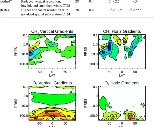
Fig. 1. Gradients of CH4 and O3 calculated from April zonal monthly means from the GSFC CTM with 2◦×2.5◦ resolution and 55

vertical levels. The vertical coordinate is pressure (hPa). Vertical gradients (left column) have units of percentage change/km (calculated for mixing ratios (upper box-lower box)×100/lower box) with negative values indicate decreasing tracer with height. Horizontal gradients (right column) have units of percentage change/4◦latitude (calculated for mixing ratios (poleward-equatorward)x100/equatorward), with positive values indicating a poleward increase. No values are calculated across the equator. White areas represent gradients of less than 5%.

to different horizontal grids, which may have lead to inaccu-racies in the vertical winds. However, each CTM came from a different institution and there was more than one difference between the simulations, for example both horizontal regrid-ding and time between meteorological updates differed, mak-ing the determination of the cause(s) of the differences inex-act. Van den Broek et al. (2003) used a CTM with the

finite-differencing advection scheme of Russell and Lerner (1981) at 3 horizontal resolutions to investigate the effect on tracer profiles in the Arctic vortex. They concluded that 6◦_×9◦ res-olution was too coarse to represent the vortex, but that 3◦_×2◦ and 1◦_×1◦_{resolution performed equally well and better than} 6◦×9◦resolution. But using a CTM with the Prather (1986) second order moments advection scheme, Searle et al. (1998)

Full Vert CH4 -50 0 50 LAT 100 10 1 PRES 300 300 450 600 800 1000 1200₁₄₀₀ 1600

CH4: Reduced Vert - Full Vert

-50 0 50 LAT 100 10 1 PRES 0 0 0 0 0 0 0 Full Vert O3 -50 0 50 LAT 100 10 1 PRES 0.1 0.2 0.5 1.0 2.0 3.0 3.0 4.0 5.0 6.0 7.0

O3: Reduced Vert - Full Vert

-50 0 50 LAT 100 10 1 Theta (K) 0.0 0.0 0.0 0.0

Full Vert Mean Age after 5 yrs

-50 0 50 LAT 100 10 1 Pres 0.5 1.01.5 2.0 2.5 3.0 3.0

Mean Age: Reduced Vert - Full Vert

-50 0 50 LAT 100 10 1 Pres 0.0 0.0 0.0 0.0 Figure 2

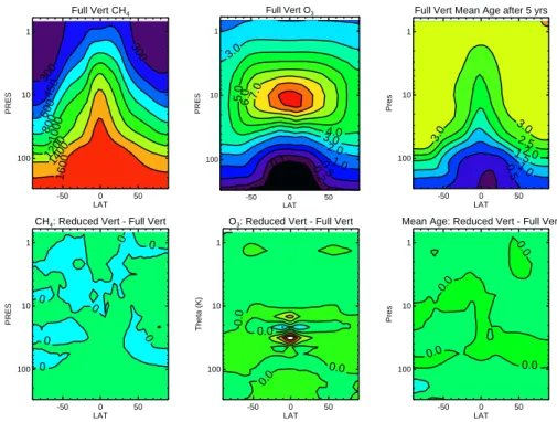
Fig. 2. Top panels: Zonal annual mean CH4(ppb) and O3(ppm), and mean age (years) in the GSFC CTM with full vertical resolution.

Bottom panels: Differences in CH4, O3, and mean age between a reduced resolution CTM and the full resolution CTM (Reduced Vert – Full

Vert). The vertical coordinate is pressure (hPa). The intervals in the difference plots are 50 ppb CH4, 0.2 ppm O3, and 0.1 year. Ozone is

sensitive to the slightly different spacing of levels in these models near its large tropical gradient.

found that transport across the vortex edge was insensitive to horizontal resolution even at 5.6◦×5.6◦. (The second order moments scheme is less diffusive because it retains higher order moment information for transport.) It is vital to un-derstand a model’s sensitivity to resolution because of the serious consequences it may have on its ability to maintain high Clylevels in the vortex and to disperse ozone-depleted

air to the midlatitudes.

Table 1 lists the series of experiments performed to test different implementations of the input meteorological fields in our CTM. Each experiment is designed to test the effect of only one thing – for example, the reduction of horizon-tal resolution – and contains a single implementation change relative to another, usually the experiment above it in the ta-ble. Some observations are used to establish the realism of the simulation’s behavior, but most comparisons are between experiments with the goal of understanding how one differs from another. The model intercomparisons presented allow us to address questions such as

– How does the vertical resolution of the input wind fields

affect the CTM transport circulation?

– What is the impact on the stratosphere of lowering the

CTM lid?

– How does horizontal resolution affect tracer transport?

3.2 Model analysis tools

Evaluation of transport sensitivity requires constituents that have significant vertical or horizontal gradients and rela-tively long photochemical lifetimes. Methane and ozone are long-lived in much of the stratosphere. Methane has a surface source and destruction in the upper stratosphere, while ozone is produced and destroyed primarily in the mid-dle and upper stratosphere. The locations of large gra-dients in CH4 and O3 are different because of the

differ-ences in their sources and sinks, but used together their gradients show sensitivity to transport over much of the stratosphere. Model vertical and horizontal gradients are shown in Fig. 1 to indicate where each constituent has the greatest transport sensitivity. Because the model CH4 and

O3 distributions are realistic compared to the UARS

ref-erence atmosphere plots (see http://code916.gsfc.nasa.gov/ Public/Analysis/UARS/urap/home.html), the model gradi-ents in Fig. 1 are representative of observed gradigradi-ents. Exam-ples of zonal mean CH4and O3fields are presented in Fig. 2.

Ozone has large sensitivity to transport across the subtropics in the lower stratosphere and CH4 is especially sensitive to

vertical motions at high latitudes. Ozone gradients are sim-ilar in all seasons while CH4gradients tend to be largest at

the mid and high latitudes during the cold seasons. Smaller transport sensitivity is seen for O3above ∼20 hPa where its

distribution is strongly influenced by photochemistry.

These species are also well suited for model evaluation because they have been extensively measured by aircraft and satellite instruments. Long-term, global data sets of CH4and

O3are available from the Halogen Occultation Experiment

(HALOE) (Park et al., 1996) and the Cryogenic Limb Array Etalon Spectrometer (CLAES) (Roche et al., 1996) on the Upper Atmosphere Research Satellite (UARS). This study uses process-oriented diagnostics derived from HALOE and CLAES measurements to evaluate how well physical pro-cesses are represented by the models. Similar diagnostics were used to evaluate transport in GMI CTM simulations (Douglass et al., 1999; Strahan and Douglass, 2004).

The behavior of the lower stratospheric Antarctic vortex in spring is examined in Fig. 8. The details and interpretation of this analysis, including a description of the HALOE data set used to derive this test, can be found in Strahan and Dou-glass (2004). The springtime CH4pdfs, one from 60◦–80◦S

(mostly vortex air, blue) and one from 44◦–60◦S (mostly midlatitude air, red), illustrate vortex isolation and the man-ner in which it erodes. The September Full Vert vortex has a sharper edge than HALOE, indicated by much greater sepa-ration of the pdfs. During November, the model and analyzed pdfs are very similar in shape, separation, and most probable value. This is interpreted as the model forming a strong vor-tex earlier than observed by HALOE, but having a realistic dynamical evolution during spring. Results for Reduced Vert are not plotted because they are indistinguishable from Full Vert. This behavior demonstrates that reduced vertical reso-lution in the middle stratosphere and above has no significant impact on the processes that maintain and erode the lower stratospheric Antarctic vortex in spring. Similar behavior is found in HALOE and the models at 600 K.

4 Offline and online calculations

The CTM and FVGCM have been integrated with the same parameterized CH4loss and surface boundary conditions but

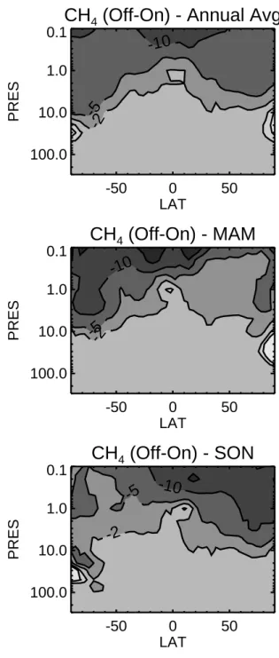
do not produce the same results. Figure 3 shows the differ-ences between the FVGCM and the CTM simulation “Full Vert”, which was integrated with the same winds and grid as the FVGCM. The annual mean differences, shown for the 5th year of the CTM simulation, which have reached a steady state, show that stratospheric CH4in the CTM is usually 1–

5% lower than the FVGCM. Previous studies have suggested that offline transport differences arise from the differences between the vertical wind in the CTM (calculated from conti-nuity using the 6-hourly averaged u and v fields) and the ver-tical wind calculated in the GCM (Rasch et al., 1994; Waugh et al., 1997). The CH4differences are greatest in the upper

atmosphere where both photochemistry and vertical transport have greater tendency terms, and where errors in the calcu-lation of either, for example due to time-averaging of winds, will increase the model differences.

CH

(Off-On) - Annual Avg

-50

0

50

LAT

100.0

10.0

1.0

0.1

PRES

-10

-5

-2

CH

(Off-On) - MAM

-50

0

50

LAT

100.0

10.0

1.0

0.1

PRES

-10

-5-2

CH

(Off-On) - SON

-50

0

50

LAT

100.0

10.0

1.0

0.1

PRES

-10

-5

-2

Figure 3

Fig. 3. Percentage difference in CH₄ distributions between the

offline CTM calculation and an online chemical calculation in a GCM ((offline-online)/online ×100%). Top to bottom: annual aver-age, March-April-May mean, and September–October–November mean. The vertical coordinate is pressure (hPa).

The other panels of Fig. 3 show the differences between online and offline during the seasons of greatest vertical transport (diabatic descent) in each hemisphere, where CH4

has large sensitivity to vertical transport. Photochemical loss is negligible at high latitudes during fall and is unlikely to be the cause of the differences. Horizontal maps (not shown)

Full Vert 100 hPa 0 20 40 60 80 100 120 DAYS -50 0 50 LAT 0.001 0.001 0.005 0.005 0.020 0.020 0.200

Reduced Vert 100 hPa

0 20 40 60 80 100 120 DAYS -50 0 50 LAT 0.001 0.001 0.005 0.005 0.020 0.020 0.200

Full Vert 10 hPa

400 420 440 460 480 500 520 540 DAYS -50 0 50 LAT 0.001 0.005 0.020

Reduced Vert 10 hPa

400 420 440 460 480 500 520 540 DAYS -50 0 50 LAT 0.001 0.001 0.0050.020 Figure 4

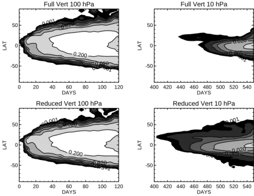
Fig. 4. Left column: Age tracer on the 100 hPa surface in Full Vert (top) and Reduced Vert (bottom) for the first year of simulation. Right

column: age tracer on the 10 hPa surface, same simulations. Full Res has 12 levels between 100 and 10 hPa but Reduced Vert has only 8.

have the greatest differences during periods of strong wave activity, which is usually accompanied by vertical motions, with near zero differences during quiescent periods. Rasch et al. (1994) and Waugh et al. (1997) speculate that the use of 6-hourly averaged u and v in the CTM leads to smaller calcu-lated vertical velocity because mixing due to large transient waves is removed by averaging. This would result in slower tropical ascent in the CTM and for a CH4-like tracer would

produce differences with the same sign as shown here.

5 Results of CTM implementation experiments

In each section below, a pair of simulations is compared to determine how the change in implementation affects strato-spheric transport processes. An overview of the circula-tion differences is presented first. Then, a series of process-oriented comparisons is made that examines tropical ascent, exchange between the tropics and midlatitudes, poleward transport of tropical air in the upper stratosphere, and the be-havior of the lower stratospheric Antarctic vortex in spring. 5.1 The effect of decreasing vertical resolution in the

stratosphere and mesosphere

This section compares CTM simulations using the original FVGCM 55 level winds (“Full Vert”) and one with 33 level wind fields (“Reduced Vert”); both models have the same lid (0.015 hPa) and horizontal resolution. The number of levels

is reduced by a process that maps the u and v wind fields to a different set of vertical levels in a way that conserves the divergence and mass flux of the vertical winds between the original levels (Lin, 2004). The resolution is very simi-lar from 225–43 hPa, but from 43–1 hPa Full Vert has twice the vertical resolution and above 1 hPa it has three times the resolution.

Figure 2 summarizes the circulation differences. The top panels show annual zonal mean distributions of CH4 and

O3, and the mean age in Full Vert after 5 years, while the

lower panels show the differences between the experiments. Methane is sensitive to vertical transport in the middle strato-sphere and above, yet the differences due to reduced resolu-tion are almost negligible. Ozone differences greater than 2% only occur in the tropical lower stratosphere in the re-gion with large vertical gradients and where there are slight differences in level spacing. Mean age differences are in-significant. (The calculation of the true mean age would re-quire a 20-year integration. After 5 years, the mean ages are asymptotically approaching their “true” value. The dif-ference between mean ages in the two simulations reaches it asymptotic limit much sooner, thus, the mean age differences after Year 4 are nearly converged.)

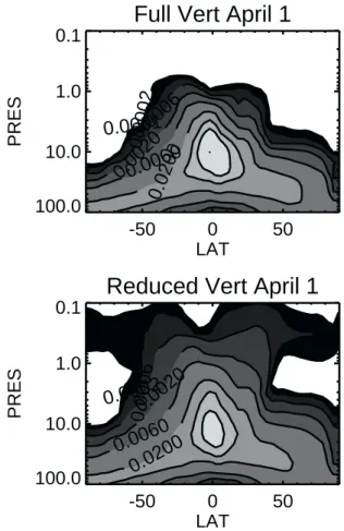
Figure 4 examines the process of ascent using the arrival of the age tracer on the 100 hPa and 10 hPa surfaces. The age tracer arrives at the tropical tropopause (100 hPa) with the same timing and distributions in both simulations. Above 56 hPa, Full Vert levels are more closely spaced and the

Full Vert April 1

-50

0

50

LAT

100.0

10.0

1.0

0.1

PRES

0.0001

0.0006

0.0002

0.0020

0.0060

0.0200

Reduced Vert April 1

-50

0

50

LAT

100.0

10.0

1.0

0.1

PRES

0.0002

0.0020

_0.0006

0.0060

0.0200

Figure 5

Fig. 5. Comparison of Full Vert (top) and Reduced Vert (bottom)

age tracer distributions near the end of the 2nd year of simulation. The vertical coordinate is pressure (hPa).

arrival time at 10 hPa shows that its ascent and meridional spread are slower. The relationship between level spacing and ascent is quite strong in the mesosphere, where Reduced Vert has only 1/3 of the levels of Full Vert. This relationship is expected because the transport spreads the tracer uniformly through the grid box, and the fewer the grid boxes, the faster the diffusion (Rood, 1987). Figure 5 shows that after nearly 2 years of simulation, the Reduced Vert age tracer has filled much more of the lower mesosphere than Full Vert.

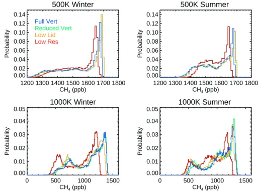
Faster ascent and poleward transport lead to stronger ex-change between tropical and midlatitude air masses. Figure 6 shows the probability distribution functions (pdfs) for CH4

between 10◦_S–46◦_{N on isentropic surfaces in the lower and} middle stratosphere. The shape of the long-lived tracer pdf indicates the distinctiveness of tropical and midlatitude air (Sparling, 2000) and was used to discriminate between me-teorological fields in GMI model evaluation tests (Douglass et al., 1999). All simulations show a minimum between the tropical and midlatitude distributions which indicates a sub-tropical barrier to mixing; this is seen in winter and sum-mer and at both levels shown. The tropical peaks at 500 K

(∼45 hPa) sort themselves by ascent rate, with slower ascent corresponding to higher CH4(less exchange with the

midlat-itudes), consistent with the age tracer comparison shown in Fig. 4. Ascent in Low Lid and Low Res will be discussed later in Sect. 5.

The annual cycle of CH4 in polar upper stratosphere is

a good diagnostic for several processes on seasonal time scales (Strahan and Douglass, 2004). Figure 7 shows a con-toured pdf time series of CH4 at 1200 K (∼5 hPa) in the

Antarctic for Reduced Vert, with an outline of Full Vert con-tours overlaying it. The contoured pdf can be interpreted as follows. From Austral summer to early fall (December– April), the most probable CH4mixing ratios decline sharply

and have little variability. These features are the result of photochemical loss, weak wave activity, and by early fall, descent. As wave activity increases in the fall (April–June), tropical upper stratospheric air with high CH4is transported

poleward. Wave activity is low in winter but increases again in spring (October–December), resulting in large variability due to transport of higher CH4air from lower latitudes.

Ul-timately the vortex is destroyed and midlatitude air high in CH4is thoroughly mixed into the polar region. The upper

stratospheric CH4 annual cycle in Reduced Vert has nearly

the same distributions as Full Vert, but shows slightly less variability. Similar results are found in the Arctic and at higher levels in the stratosphere. Although Fig. 5 showed that Reduced Vert has rapid mesospheric transport, because mesospheric CH4values do not differ much between the

sim-ulations, these transport differences do not impact CH4in the

upper stratosphere. We will see later that it is the presence of a lid near the mesopause that matters to stratospheric CH4.

5.2 The effect of lowering the model lid without decreasing stratospheric resolution

This section compares the 33 level simulation having a 0.015 hPa lid, referred to as Reduced Vert in the previous sec-tion, with a 28 level version having a lower lid (0.4 hPa). The lowest 27 levels of these simulations (surface to 1.33 hPa) are identical, as are their horizontal resolutions. In this section, Reduced Vert will be referred to as “High Lid” and the 28 level model will be called “Low Lid” in order to emphasize their difference.

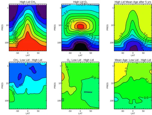
Figure 9 summarizes the mean circulation differences in the same way as Fig. 2. Lowering the lid has a much greater effect than reducing the vertical resolution above 43 hPa. Low Lid has roughly 1% higher CH4 in the lower

strato-sphere but 10–30% less CH4in the upper stratosphere. This

is consistent with the pattern of mean age differences: the air is younger where CH4is higher and older where CH4is

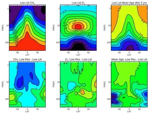
lower. In contrast to CH4, O3and age are more strongly

af-fected by the lower lid in the southern hemisphere (SH). High Lid has low ozone in the mesosphere that descends to the up-per stratosphere during late summer and fall. The absence of a source of low ozone in Low Lid is probably the reason for

500K Winter 1200 1300 1400 1500 1600 1700 1800 CH₄ (ppb) 0.00 0.02 0.04 0.06 0.08 0.10 0.12 0.14 Probability Full Vert Reduced Vert Low Lid Low Res 500K Summer 1200 1300 1400 1500 1600 1700 1800 CH₄ (ppb) 0.00 0.02 0.04 0.06 0.08 0.10 0.12 0.14 Probability 1000K Winter 0 500 1000 1500 CH4 (ppb) 0.00 0.01 0.02 0.03 0.04 0.05 Probability 1000K Summer 0 500 1000 1500 CH4 (ppb) 0.00 0.01 0.02 0.03 0.04 0.05 Probability Figure 6

Fig. 6. Probability distribution functions (pdfs) of CH₄at 500 K (top panels) and 1000 K (bottom panels) in winter (left) and summer (right)

for 4 CTM simulations. Full Vert (blue), Reduced Vert (green), and Low Lid (orange) all have 2◦×2.5◦resolution. The peak separation of Low Res (4◦×5◦, red) differs from the higher resolution models.

Reduced Vert 72-80S, 1200K

Full Vert (overlay)

Figure 7

Fig. 7. The annual cycle of model CH₄72–80◦S on the 1200 K

surface using contoured pdfs. Yellow and red are high values of the most probable mixing ratio, and purple and blue indicate low probability, or infrequently observed mixing ratios. Reduced Vert is shown in color and the outline of the mean (solid) and range (dashed) for Full Vert is overlaid.

its higher ozone in the polar upper stratosphere. (Methane has very small vertical gradients in this region and is thus insensitive here.) The lack of a full mesosphere has a neg-ligible effect on middle and lower stratospheric ozone in the

northern hemisphere (NH) in this particular winter. This is consistent with trajectory analyses of Rosenfield and Schoe-berl (2001) that showed that the composition of the Arctic lower stratospheric vortex is often, though not always, com-posed of air of middle and upper stratospheric origin, while the Antarctic vortex generally contains a significant contri-bution from mesospheric air.

The age tracer at 31 hPa (not shown) is nearly identi-cal at all latitudes in the two simulations, implying that the mesospheric lid height has little effect on middle and lower stratospheric tropical ascent and meridional transport. This is consistent with the identical tropical-midlatitude separa-tions at 500 K shown in Fig. 6 (green and yellow). Figure 6 shows small differences due to the lid height have appeared at 1000 K (∼8 hPa).

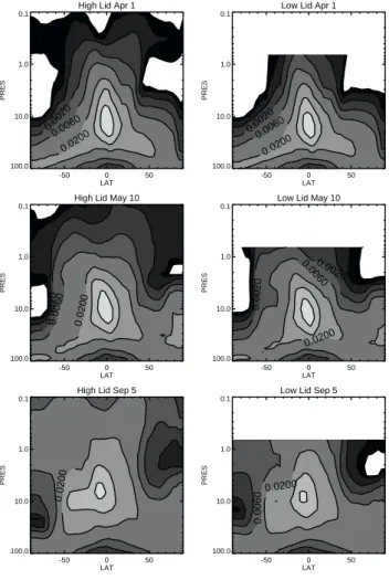
Figure 10 shows latitude-height cross-sections of zonal mean age tracer for High Lid and Low Lid on three dates in the 2nd and 3rd years of the simulations. High Lid produces the two-lobed circulation in the mesosphere (1 April and 10 May), consistent with CH4structures seen by

HALOE (Ruth et al., 1997) near equinox. This circula-tion fills the lower mesosphere, and when cooling begins in the Austral fall, poleward and downward transport of air from the lower mesosphere fills the Antarctic upper strato-sphere. By 10 May, horizontal transport near 1 hPa has brought the tracer to the Antarctic in High Lid while similar transport is clearly lacking in Low Lid. The bottom panels

(5 September) illustrate how the missing mesospheric circu-lation has a similar effect as the Arctic vortex is forming. Without a mesospheric circulation, the upper stratospheric transport is “short-circuited” in Low Lid and the Arctic up-per stratosphere is still completely isolated after more than 2 years. Having a lid near the mesopause (∼0.01 hPa) results in more effective constituent transport in the upper stratosphere. Differences in equator-to-pole transport in these models are also observed in the CH4 polar upper stratospheric

an-nual cycle (contoured pdfs) shown in Fig. 11. Pdfs of CLAES measurements during 5 southern hemispheric view-ing periods (∼35 days each) are overlaid on the model re-sults with black contours; the innermost contour indicates the most probable value. Both simulations show large vari-ability associated with the breakdown of the vortex in late spring (October–November) and a rapid decline throughout the summer (December–April). Neither simulation main-tains high CH4 up to mid-summer as shown in the

obser-vations. Both CLAES and the models show a minimum in the annual cycle in April, but by winter, only CLAES and High Lid show increased CH4resulting from strong transport

from lower latitudes. Weak upper stratospheric poleward transport in “Low lid” is indicated by persistently low CH4

from May–September; this is also shown by the age tracer in Fig. 10 (10 May). Arctic CH4in High Lid is systematically

higher in the upper stratosphere than Low Lid, but CLAES CH4is higher still, suggesting that neither model has strong

enough horizontal transport in the NH upper stratosphere. In the SH, High Lid compares very closely with CLAES, ex-cept in early summer, suggesting that the upper mesospheric lid is important for producing realistic transport in the upper stratosphere.

Although Low Lid has too little upper stratospheric CH4

in the fall, by late winter it has too much in the Antarctic lower stratosphere, consistent with the pattern of general cir-culation differences seen in Fig. 9. The differences caused by the lid are greatest in the Antarctic vortex, as seen in Figs. 9 and 12. In Fig. 12, the midlatitude distributions of the two simulations are indistinguishable, but the vortex pdf in Low Lid has much higher CH4. Air descending in the Low Lid

vortex is subject to stronger horizontal transport in the mid-dle stratosphere and below, resulting in higher CH4that

de-scends to the lower stratospheric vortex by the end of winter. Both simulations show vortex and midlatitude distributions that remain isolated from each other in spring, in good agree-ment with the analysis of HALOE CH4behavior in Strahan

and Douglass (2004). Vortex isolation is slightly better in High Lid. High Lid vortex pdfs in September and November (solid blue lines) have greater overlap (53%) than Low Lid vortex pdfs (dashed blue lines, 41%). That is, the Low Lid vortex pdfs change more during spring because more midlat-itude air is able to mix in. Similar differences in behavior are found are found in the NH.

Sep 450K

400 600 800 10001200140016001800

CH

(ppb)

0.00

0.02

0.04

0.06

0.08

0.10

0.12

0.14

Probability

Vortex

Surf Zone

___ Full Vert

- - - HALOE

Nov 450K

400 600 800 10001200140016001800

CH

(ppb)

0.00

0.02

0.04

0.06

0.08

0.10

0.12

0.14

Probability

Vortex

Surf Zone

___ Full Vert

- - - HALOE

Figure 8

Fig. 8. Comparison of the separation of vortex (60–80◦S, blue)

and midlatitude (44–60◦S, red) air masses in Full Vert (solid) and HALOE (dashed) CH4in September and November. Full Vert has

a sharper vortex edge in September than seen by HALOE, but by November, model and observed vortex and midlatitude air masses distributions are very similar. Pdfs from Reduced Vert (not shown) are indistinguishable from Full Vert.

5.3 The effect of lower horizontal resolution

This section compares the simulations “Low Res” and “Low Lid” which have the same 28 vertical levels and 0.4 hPa lid but different horizontal resolution. The Low Res 4◦×5◦wind fields were created by subsampling the Low Lid 2◦×2.5◦ fields.

The comparison of mean CH4, O3, and age differences

in Fig. 13 shows that decreased horizontal resolution has a much greater effect than reduced vertical resolution or low-ering the CTM lid. In the Low Res lower stratosphere, lower CH4at low latitudes and higher CH4 at high latitudes (i.e.,

flatter meridional gradients) suggest that lower horizontal resolution leads to increased horizontal mixing. Higher O3in

High Lid CH4 -50 0 50 LAT 100 10 1 PRES 300 300 450 600 800 1000 1200₁₄₀₀ 1600

CH4: Low Lid - High Lid

-50 0 50 LAT 100 10 1 PRES 0 -50 50 High Lid O3 -50 0 50 LAT 100 10 1 PRES 0.1 0.2 0.5 1.0 2.0 2.0 3.0 3.0 4.0 5.06.0 7.0

O3: Low Lid - High Lid

-50 0 50 LAT 100 10 1 PRES 0.0 0.2

High Lid Mean Age after 5 yrs

-50 0 50 LAT 100 10 1 PRES 0.5 1.01.5 2.0 2.5 3.0 3.0

Mean Age: Low Lid - High Lid

-50 0 50 LAT 100 10 1 PRES 0.0 0.1 0.2 Figure 9

Fig. 9. Top panels: Zonal annual mean CH4and O3, and mean age in High Lid (Reduced Vert). Bottom panels: Differences in CH4, O3,

and mean age between Low Lid and High Lid (Low Lid – High Lid). The vertical coordinate is pressure (hPa). The intervals in the differnce plots are 50 ppb CH₄, 0.2 ppm O₃and 0.1 year.

transport out of the tropical production region. The patterns of age and CH4differences are very similar. With young air

more likely to circulate poleward than upward in Low Res, the middle stratosphere and above are “depleted” in young air, increasing the mean age there and decreasing the age in the polar lower stratosphere. The mean age comparisons shown in Figs. 3, 9, and 13 show that lowering the lid or decreasing the horizontal resolution noticeably compromises transport, making it harder for air to get to the middle strato-sphere and above, but easier to mix poleward below that.

These circulation problems are easily traced to several transport processes. Figure 14 shows age spectra in the polar lower stratosphere (57 hPa) and near the tropical O3

maxi-mum (10 hPa) from four CTM simulations. The Low Res age is markedly different from all the 2◦×2.5◦ age spectra, especially in the southern hemisphere. In the polar lower stratosphere, Low Res air arrives much sooner and continu-ously, rather than having an annual cycle of transport as seen in all other implementations. In the tropical middle strato-sphere, it arrives at 10 hPa before the others but there is less of it because more has mixed out of the tropics before arriv-ing there.

Figure 14 demonstrates that 4◦×5◦resolution allows too much leakage out of the lower stratospheric tropical pipe and explains the structure of the mean age difference in Fig. 13. Low Res allows greater mixing of young and old (midlati-tude) air in the lower stratosphere, making the tropics older

and the extratropics younger, and results in slightly older air ascending to the middle and upper stratosphere. This effect was also seen in Fig. 6, where the Low Res 500 K tropical and midlatitude peaks are shifted toward each other (more mixing) compared to the 2◦×2.5◦ simulations. At 1000 K (above 10 hPa), both peaks are shifted to lower mixing ra-tios, reflecting the difficulty of getting young air above the tropical lower stratosphere in the 4◦×5◦model.

The excessive horizontal mixing in Low Res actually com-pensates for the inadequate upper stratospheric equator-to-pole transport caused by the lower lid (Fig. 11), demonstrat-ing that two wrongs can appear to make a right. Figure 15 shows how meridional gradients of CH4in the upper

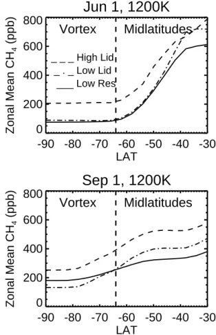
strato-sphere are affected by the change in horizontal resolution and lid during Austral winter. In June, the strongest gradients are between 40–60◦S and are similar in all 3 simulations shown. By September, the two 2◦×2.5◦ simulations show parallel gradients at the vortex edge while the 4◦×5◦is weaker. Fig-ure 11 showed that CH4in the upper stratospheric vortex at

the end of winter was simulated well by High Lid but was too low in Low Lid. Figure 15 shows that Low Res moderates the low vortex values seen in Low Lid; unfortunately, this im-provement is caused by the inability of Low Res to maintain a vortex edge gradient and the improved vortex agreement comes at the expense of midlatitude values.

The behavior of the Low Res Antarctic vortex demon-strates a serious consequence of decreased horizontal

High Lid Apr 1 -50 0 50 LAT 100.0 10.0 1.0 0.1 PRES 0.0020 0.0060 0.0200

Low Lid Apr 1

-50 0 50 LAT 100.0 10.0 1.0 0.1 PRES 0.0020_0.0060 0.0200

High Lid May 10

-50 0 50 LAT 100.0 10.0 1.0 0.1 PRES 0.00200.0060 0.0200

Low Lid May 10

-50 0 50 LAT 100.0 10.0 1.0 0.1 PRES 0.0020 0.0020 0.0060 0.0200

High Lid Sep 5

-50 0 50 LAT 100.0 10.0 1.0 0.1 PRES 0.0200

Low Lid Sep 5

-50 0 50 LAT 100.0 10.0 1.0 0.1 PRES 0.0060 0.0200 Figure 10

Fig. 10. Zonal mean age tracer distributions for High Lid (left

pan-els) and Low Lid (right panpan-els) for 1 April (day 641), 10 May (day 680), and 5 September (day 797). The vertical coordinate is pres-sure (hPa). Lacking a mesopheric pathway, Low Lid transports air to the polar upper stratosphere much more slowly.

resolution. Consistent with Fig. 15, Fig. 16 shows that 450 K vortex and midlatitude air masses in September are less sep-arated at 4◦×5◦than at 2◦×2.5◦. In spite of too little CH4in

Low Res in the Antarctic upper stratosphere in fall, its exces-sive horizontal mixing results in too much CH4in the lower

stratosphere by spring. By November, the Low Res vortex air mass has significantly increased mixing ratios compared to Low Lid. The overlap between the September and Novem-ber vortex distributions indicates how much the vortex air has changed. Low Res has only 19% overlap, compared to 41% for Low Lid and 53% for High Lid, indicating considerable incorporation of midlatitude air by Low Res. In November, Low Res pdfs are overlapped and the vortex peak has in-creased by ∼200 ppb since September. This contrasts with the Full Vert vortex peak change of about +50 ppb during spring. The lack of a strong barrier to mixing has impor-tant consequences for the maintenance of the high Cly/low NOx environment required to successfully simulate

Antarc-High Lid 72-80S, 1200K

J F M A M J J A S O N D J

0

200

400

600

800

CH

(ppb)

___ CLAES

Low Lid 72-80S, 1200K

J F M A M J J A S O N D J

0

200

400

600

800

CH

(ppb)

___ CLAES

Figure 11

Fig. 11. The annual cycle of CLAES and model CH₄72–80◦S on

the 1200 K surface using contoured pdfs. Yellow and red are high values of the most probable mixing ratio, and purple and blue indi-cate low probability, or infrequently observed values. CLAES pdfs from 5 southern hemisphere viewing periods are overlaid on the High Lid (top) and Low Lid (bottom) annual cycles. The innermost contours of the CLAES pdfs are the most probable values.

tic ozone depletion, and for the dispersion of ozone-depleted air into the midlatitudes.

5.4 Requirements for producing a realistic vortex edge Was the leaky vortex behavior of Low Res caused by the 4◦×5◦resolution of the advection calculation? Or, is forc-ing at scales smaller than 4◦×5◦ essential to forming and maintaining the vortex? If it is a resolution effect, do we know that advection at 2◦_×2.5◦ _{is adequate? These} ques-tions are addressed with two additional experiments. One experiment is run at 2◦×2.5◦resolution, but uses the 4◦×5◦ winds that were linearly interpolated back to 2◦×2.5◦ and thus contain no wave forcing below the scale of the 4◦×5◦ grid (“Smoothed”). The other experiment uses the origi-nal 2◦×2.5◦winds linearly interpolated to 1◦×1.25◦(“High Res”) and thus contains no wave forcing below the scale of the 2◦×2.5◦winds (Low Lid). We address the issue of

Sep 450K

600 800 10001200140016001800

CH

(ppb)

0.00

0.02

0.04

0.06

0.08

0.10

Probability

Vortex

Surf Zone

___ High Lid

- - - Low Lid

Nov 450K

600 800 10001200140016001800

CH

(ppb)

0.00

0.02

0.04

0.06

0.08

0.10

Probability

Vortex

Surf Zone

Figure 12

Fig. 12. Comparison of the separation of vortex (60–80◦S, blue)

and midlatitude (44–60◦S, red) air masses in High Lid (solid) and Low Lid (dashed) in September and November. The lid height does not affect the midlatitude distributions, but the High Lid vortex maintains lower CH4.

producing a realistic vortex edge by comparing these new experiments with Low Lid and Low Res. These results are specific to the Lin and Rood (1996) advection scheme used in this CTM; Searle et al. (1998) found that the sensitivity to resolution depends on the diffusiveness of the advection scheme.

What makes the Low Lid vortex behavior more realistic than Low Res? The top panels of Fig. 17 compare the state of the November vortex in Low Res (top) and Low Lid (middle) with an intermediate experiment, “Smoothed”, which has 2◦_×2.5◦_{advection but 4}◦_×5◦_{information content. All} simu-lations were begun on 1 July from the same initial conditions. The top panel shows that Low Res and Smoothed do not get the same CH4distributions even though the winds have the

same scale wave forcings, implying that resolution matters in the formation of the vortex mixing barrier. In the middle panel, the experiments have the same 2◦×2.5◦advection but different information content in the winds. The experiments’ pdfs are nearly identical, suggesting that smaller scale waves do not play an important role in vortex behavior. This is

con-sistent with the results of Waugh and Plumb (1994) showing that small scale atmospheric structures could be produced from low resolution wind fields. Realistic vortex behavior is impaired by the 4◦×5◦resolution in this CTM, but not by the lack of small scale wave forcing.

The bottom panel of Fig. 17 compares the 2◦×2.5◦ ad-vection of “Low Lid” with an experiment using the Low Lid winds interpolated to 1◦×1.25◦(“High Res”). The winds in High Res have the same information content as Low Lid. The differences in the shapes, peaks, and separations of the vortex and midlatitude pdfs are very slight, with High Res having a slightly stronger barrier to mixing (i.e., lower vortex CH4).

The top panel demonstrates a significant improvement in vor-tex behavior going from 4◦×5◦to 2◦×2.5◦, while the bottom panel shows very little gain in vortex isolation at 1◦×1.25◦ resolution. (Since the original resolution of the FVGCM is 2◦×2.5◦, we cannot say whether a higher resolution GCM might produce a better vortex.)

6 Summary: Implementation effects on transport pro-cesses

A chemistry and transport model using stored meteorologi-cal fields is a useful tool that can make complex atmospheric studies tractable. It is essential that we understand how our implementation choices affect the results calculated. To that end, this paper has examined the representation of strato-spheric processes using a variety of implementations to iden-tify the consequences of lowering the CTM lid, the vertical resolution, and the horizontal resolution.

Realistic tropical ascent in models is important for simu-lating the propagation of an annually varying cycle into the stratosphere, for example, the “tape recorder” in water (Mote et al., 1996). The rate of ascent was affected by level spac-ing, with more closely spaced levels leading to slower ascent. This could be caused by vertical diffusion (i.e., air can dif-fuse faster when it has fewer grid boxes to travel through), or it could result from the method of mapping the original wind fields to lower vertical resolution. Mesospheric lid height had no impact on ascent rate below the middle stratosphere, but a low lid slowed ascent slightly in the upper stratosphere. Hor-izontal resolution affected ascent, with the Low Res (4◦×5◦)

simulation having faster ascent than all the 2◦×2.5◦ simula-tions (Fig. 14).

The strength of the subtropical mixing barrier is relevant to the impact of lower stratospheric midlatitude aircraft emis-sions on tropical ozone (Douglass et al., 1999). All CTM ver-sions produced some barrier to tropical-midlatitude exchange in the middle and lower stratosphere, but the barrier was no-ticeably weaker at 4◦×5◦resolution. The simulation with the slowest ascent also had the strongest barrier to mixing with the midlatitudes. Surprisingly, the simulation with faster ascent also had older mean age in the upper stratosphere

Low Lid CH4 -50 0 50 LAT 100 10 1 PRES 300 300 450 600 800 1000 1200 1400 1600

CH4: Low Res - Low Lid

-50 0 50 LAT 100 10 1 PRES -100 -50 0 0 50 50 Low Lid O3 -50 0 50 LAT 100 10 1 PRES 0.1 0.2 0.51.0 2.0 3.0 3.0 4.0 5.0 6.0 7.0 8.0

O3: Low Res - Low Lid

-50 0 50 LAT 100 10 1 PRES 0.0 0.0 0.0 0.2

Low Lid Mean Age after 5 yrs

-50 0 50 LAT 100 10 1 PRES 0.5 1.01.5 2.0 2.5 3.0 3.5 3.5

Mean Age: Low Res - Low Lid

-50 0 50 LAT 100 10 1 PRES -0.1 0.0 0.0 0.1 Figure 13

Fig. 13. Top panels: Zonal annual mean CH4and O3, and mean age in the GSFC CTM with reduced vertical resolution and low lid (Low

Lid). Bottom panels: Differences in CH₄, O₃, and mean age between a 4◦×5◦resolution CTM (Low Res) and the 2◦×2.5◦resolution Low Lid. The vertical coordinate is pressure (hPa). The Low Res tropical pipe is not as isolated and poleward transport is much stronger in the lower stratosphere. The intervals in the differnce plots are 50 ppb CH₄, 0.2 ppm O₃and 0.1 year.

because of the concomitant strong tropical-midlatitude ex-change that aged the tropical air.

Douglass et al. (2004) demonstrated that transport is im-portant for the simulation of upper stratospheric ozone be-cause the distribution of NOyand ClOxfamilies, which pro-vide the primary losses for O3, are controlled by transport.

Polar upper stratospheric transport was not significantly af-fected by a reduction in vertical levels above the middle stratosphere. However, moving the lid from 0.01 hPa to 0.4 hPa did have a significant effect. The lack of a full meso-sphere in Low Lid inhibited transport of air from low to high latitudes, leading to a more isolated polar upper stratosphere. With a low lid and 4◦×5◦resolution, the CTM compensated for weak transport in the polar upper stratosphere by en-hanced horizontal mixing. Stronger horizontal mixing flat-tened the high latitude gradients, ‘correcting’ the low CH4in

the polar region. This correction was cosmetic only and did not improve the physical representation.

The behavior of the Antarctic vortex is clearly very im-portant to simulations of the ozone hole, including those that predict its future disappearance. The reduction of vertical resolution above the lower stratosphere had a negligible ef-fect on the behavior of the Antarctic vortex during spring, but lowering the lid increased poleward horizontal transport and mixing in the middle stratosphere. Low Lid allowed slightly greater mixing between the vortex and midlatitudes.

Lower-ing the horizontal resolution to 4◦×5◦produced a weak bar-rier, with significant mixing between vortex and midlatitude air masses throughout spring. The results of an experiment run at 2◦×2.5◦with small scale wind structure removed de-termined that the poor vortex edge behavior was caused by the 4◦×5◦advection and not by a lack of small scale winds. A further experiment at 1◦×1.25◦resolution showed only a small increase in vortex isolation. Realistic containment of perturbed chemistry inside the vortex is possible in this CTM integrated at 2◦_×2.5◦_{, but not at lower resolution.}

The sensitivity to lid height was not the same in the Arc-tic and AntarcArc-tic lower stratosphere. The age spectra of all the 2◦×2.5◦simulations were nearly identical in the Arctic, while in the Antarctic, the low lid model differed from both high lid models and indicated a greater influence from young air. This shows the need for a full mesosphere to represent the Antarctic stratosphere, not just because the mesosphere is a source of old air, but because the vortex mixing barrier is slightly better represented with a high lid. The simulation of Arctic lower stratospheric phenomena requires 2◦×2.5◦, but some Arctic winters could be well represented without a full mesosphere or high vertical resolution above 50 hPa.

Low horizontal resolution compromises the model’s abil-ity to confine chemically perturbed air (e.g., high Cly and low NOx), which is especially important in the Antarc-tic vortex in September when ozone loss is rapid. This

2S, 10 hPa

0

1

2

3

4

5

Years

0.000

0.005

0.010

0.015

Age Tracer

Full Vert

Reduced Vert

Low Lid

Low Res

74S, 57 hPa

0

1

2

3

4

5

Years

0.000

0.002

0.004

0.006

0.008

Age Tracer

74N, 57 hPa

0

1

2

3

4

5

Years

0.000

0.001

0.002

0.003

0.004

0.005

0.006

Age Tracer

Figure 14

Fig. 14. Five-year age spectra in the tropical middle stratosphere

(top), and Antarctic (middle) and Arctic (bottom) lower stratosphere from 4 simulations. In the middle stratosphere, the simulation with the highest (lowest) spatial resolution (Full Vert, blue and Low Res, red) has the slowest (fastest) tropical ascent with the greatest (least) tropical isolation. Low Lid shows transport differences from the high lid simulations in the Antarctic but not in the Arctic.

conclusion applies to the Lin and Rood advection scheme used here. Searle et al. (1998) saw no sensitivity of po-lar ozone loss to horizontal resolution that ranged from 1.4◦×1.4◦ to 5.6◦×5.6◦ in their CTM using a second

or-Jun 1, 1200K

-90 -80 -70 -60 -50 -40 -30

LAT

0

200

400

600

800

Zonal Mean CH

(ppb)

Vortex

Midlatitudes

Sep 1, 1200K

-90 -80 -70 -60 -50 -40 -30

LAT

0

200

400

600

800

Zonal Mean CH

(ppb)

Vortex

Midlatitudes

Figure 15

Fig. 15. Methane meridional gradients in the SH for High Lid

(dashed), Low Lid (dot-dash), and Low Res (solid). The gradients of the three simulations are similar in late fall (top), but by the end of winter (bottom), the Low Res gradient between the midlatitudes and the vortex is much flatter than the two 2◦×2.5◦simulations.

der moments advection scheme (Prather, 1986), which is less diffusive because it carries more information about the con-stituent distribution within each gridbox; they did find less ozone loss as resolution decreased in a more diffusive ad-vection scheme (Williamson and Rasch, 1989). Our CTM implementation results are consistent with the analyses of two 4◦×5◦ simulations with the GMI CTM (Considine et al., 2004). In the Antarctic, they found that high Cly was not maintained long enough and ozone loss was not fast enough to sufficiently deplete ozone in simulations integrated at 4◦×5◦. Improvement in the containment of perturbed chemistry in the GSFC CTM integrated at 2◦×2.5◦ resolu-tion has been seen in a recent 50-yr CTM simularesolu-tion of ozone recovery (Stolarski et al., 2006).

The experiments presented here show that a faithful repre-sentation of stratospheric transport in this CTM using Lin and Rood advection is possible with relatively low verti-cal resolution (>4 km spacing) in the middle stratosphere and above, but lowering the lid from the upper to lower

Sep 450K

600 800 10001200140016001800

CH

(ppb)

0.00

0.02

0.04

0.06

0.08

0.10

Probability

Vortex

Surf Zone

__ 2x2.5

- - 4x5

Nov 450K

600 800 10001200140016001800

CH

(ppb)

0.00

0.02

0.04

0.06

0.08

0.10

Probability

Vortex

Surf Zone

Figure 16

Fig. 16. Comparison of the separation of vortex (60–80◦S, blue)

and midlatitude (44–60◦S, red) air masses in Low Lid (solid) and Low Res (dashed) in September and November. The large shift in Low Res vortex mixing ratios indicates vortex isolation is compro-mised by low horizontal resolution.

mesosphere has consequences for the realism of upper strato-sphere. This ultimately has an effect on the polar lower stratosphere, but more so for the Antarctic than the Arctic. The fidelity of lower stratospheric transport is strongly de-pendent on the presence of realistic mixing barriers in both the subtropics and high latitudes, and thus requires 2◦×2.5◦ resolution. The ability of CTMs to quickly perform sensi-tivity studies such as these makes them a valuable tool for climate and chemistry assessments and in the development of thoroughly evaluated, credible chemistry-climate models. Acknowledgements. We thank S. Pawson of the Goddard Modeling

and Assimilation Office for providing FVGCM model output for the CTM integrations, and A. Douglass for helpful discussions. This work was funded by the NASA Modeling, Analysis, and Prediction Program.

Edited by: P. Haynes

4x5 vs. 2x2.5 Advection

1000

1200

1400

1600

1800

CH

(ppb)

0.00

0.05

0.10

0.15

0.20

Probability

60-80S

40-60S

Both 2x2.5 Advection

1000

1200

1400

1600

1800

CH

(ppb)

0.00

0.05

0.10

0.15

0.20

Probability

60-80S

40-60S

2x2.5 vs. 1x1.25 Advection

1000

1200

1400

1600

1800

CH

(ppb)

0.00

0.05

0.10

0.15

0.20

Probability

60-80S

40-60S

Figure 17

Fig. 17. The effects of advection resolution and small scale winds

on vortex behavior, demonstrated with the evolution of vortex and midlatitude CH4 pdfs. Top: simulations with different horizontal

resolution but same scale forcing in the wind fields (4◦×5◦). Mid-dle: simulations with the same resolution (2◦×2.5◦)but different scale forcing in the wind fields. Bottom: simulations with differ-ent horizontal resolution but same scale forcing in the wind fields (2◦×2.5◦).

References

Austin, J.: A three-dimensional coupled chemistry-climate model simulation of past stratospheric trends, J. Atmos. Sci., 59, 218– 232, 2002.

Austin, J. and Butchart, N.: Coupled chemistry-climate model sim-ulations for the period 1980 to 2020: Ozone depletion and the start of ozone recovery, Q. J. R. Meteorol. Soc., 129, 3225–3249, 2003.

Bregman, A., Krol, M. C., Teyssedre, H., Norton, W. A., Iwi, A., Chipperfield, M., Pitari, G., Sundet, J. K., and Lelieveld, J.: Chemistry-transport model comparison with ozone observations in the midlatitude lowermost stratosphere, J. Geophys. Res., 106, 17 479–17 496, 2001.

Considine, D. B., Connell, P. S., Bergmann, D. J., Rotman, D. A., and Strahan, S. E.: Sensitivity of Global Modeling Ini-tiative model predictions of Antarctic ozone recovery to in-put meteorological fields, J. Geophys. Res., 109, D15301, doi:10.1029/2003JD004487, 2004.

Douglass, A. R., Prather, M. J., Hall, T. M., Strahan, S. E., Rasch, P. J., Sparling, L. C., Coy, L., and Rodriguez, J. M.: Choosing me-teorological input for the global modeling initiative assessment of high-speed aircraft, J. Geophys. Res., 104, 27 545–27 564, 1999.

Douglass, A. R., Schoeberl, M. R., Rood, R. B., and Pawson, S.: Evaluation of transport in the lower tropical stratosphere in a global chemistry and transport model, J. Geophys. Res., 108, 4259, doi:10.1029/2002JD002696, 2003.

Douglass, A. R., Stolarski, R. S., Strahan, S. E., and Connell, P. S.: Radicals and reservoirs in the GMI chemistry and transport model: Comparison to measurements, J. Geophys. Res., 109, D16302, doi:10.1029/2004JD004632, 2004.

Fleming, E. L., Jackman, C. H., Stolarski, R. S., and Considine, D. B.: Simulation of stratospheric tracers using an improved em-pirically based two-dimensional model transport formulation, J. Geophys. Res., 104, 23 911–23 934, 1999.

Hall, T. M., Waugh, D. W., Boering, K. A., and Plumb, R. A.: Evaluation of transport in stratospheric models, J. Geophys. Res., 104, 18 815–18 839, 1999.

IPCC: Climate Change 2001: The scientific basis, The third assess-ment report of the Intergovernassess-mental Panel on Climate Change, Cambridge University Press, Cambridge, UK, 2001.

Lin, S.-J. and Rood, R. B: Multidimensional flux form semi-Lagrangian transport schemes, Mon. Wea. Rev., 124, 2046– 2070, 1996.

Lin, S.-J.: A vertically Lagrangian finite-volume dynamical core for global models, Mon Wea. Rev., 132, 2293–2307, 2004. MacKenzie, I. A. and Harwood, R. S.: Arctic ozone destruction

and chemical-radiative interaction, J. Geophys. Res., 105, 9033– 9051, 2000.

Mote, P. W., Rosenlof, K. H., McIntyre, M. C., et al.: An atmo-spheric tape recorder: The imprint of tropical tropopause tem-peratures on stratospheric water vapor, J. Geophys. Res., 101, 3989–4006, 1996.

Park, J. H., Gordley, L. L., Drayson, S. R., et al.: Validation of halo-gen occultation experiment CH4measurements from the UARS,

J. Geophys. Res., 101, 10 183–10 205, 1996.

Plumb, R. A.: A “tropical pipe” model of stratospheric transport, J. Geophys. Res., 101, 3957–3972, 1996.

Prather, M. H.: Numerical advection by conservation of second-order moments, J. Geophys. Res., 91, 6671–6681, 1986. Rasch, P. J., Tie, X., Boville, B. A., and Williamson, D. L.: A

three-dimensional transport model for the middle atmosphere, J. Geo-phys. Res., 99, 999–1017, 1994.

Roche, A. E., Kumer, J. B., Nightingale, J. L., et al.: Validation of CH4and N2O measurements by the CLAES instrument on

the Upper Atmosphere Research Satellite, J. Geophys. Res., 101, 9679–9710, 1996.

Rood, R. B.: Numerical advection algorithms and their role in at-mospheric transport and chemistry models, Rev. Geophys., 25, 71–100, 1987.

Rosenfield, J. E. and Schoeberl, M. R.: On the origin of polar vortex air, J. Geophys. Res., 106, 33 485–33 497, 2001.

Rotman, D. A., Tannahill, J. R., Kinnison, D. E., et al.: Global Modeling Initiative assessment model: Model description, inte-gration, and testing of the transport shell, J. Geophys. Res., 106, 1669–1691, 2001.

Russell, G. L. and Lerner, J. A.: A new finite-differencing scheme for the tracer transport equation, J. Appl. Meteorol., 20, 1483– 1298, 1981.

Ruth, S., Kennaugh, R., and Gray, L. J.: Seasonal, semiannual, and interannual variability seen in measurements of methane made by the UARS Halogen Occultation Experiment, J. Geo-phys. Res., 102, 16 189–16 199, 1997.

Searle, K. R., Chipperfield, M. P., Bekki, S., and Pyle, J. A.: The impact of spatial averaging on calculated polar ozone loss, 1. Model experiments, J. Geophys. Res., 103, 25 397–25 408, 1998. Sparling, L.: Statistical perspectives on stratospheric transport, Rev.

Geophys., 38, 417–436, 2000.

Strahan, S. E. and Douglass, A. R.: Evaluating the credibility of transport processes in simulations of ozone recovery using the Global Modeling Initiative three-dimensional model, J. Geophys. Res., D05110, doi:10.1029/2003JD004238, 2004.

Stolarski, R. S., Douglass, A .R., Steenrod, S. D., and Pawson, S.: Trends in stratospheric ozone: Lessons learned from a 3-D chem-ical transport model, J. Atmos. Sci., 63, 1028–1041, 2006. Tian, W. S. and Chipperfield, M. P.: A new coupled

chemistry-climate model for the stratosphere: The importance of coupling for future O₃-climate predictions, Q. J. R. Meteorol. Soc, 131, 281–303, 2005.

Van den Broek, M. M. P., van Aalst, M. K., Bregman, A., et al.: The impact of model grid zooming on tracer transport in the 1999/2000 Arctic polar vortex, Atmos. Chem. Phys., 3, 1833– 1847, 2003,

http://www.atmos-chem-phys.net/3/1833/2003/.

Waugh, D. W. and Plumb, R. A.: Contour advection with surgery: A technique for investigating finescale structure in tracer transport, J. Atmos. Sci, 51, 530–540, 1994.

Waugh, D. W., Hall, T. M., Randel, W. J., et al.: Three-dimensional simulations of long-lived tracer using winds from MACCM2, J. Geophys. Res., 102, 21 493–21 513, 1997.

Williamson, D. L. and Rasch, P. J.: Two-dimensional semi-Lagrangian transport with shape preserving interpolation, Mon. Wea. Res., 117, 102–129, 1989.